Two-layer competitive based Hopfield neural
network for medical image edge detection
Chuan-Yu Chang*
Pau-Choo Chung*
National Cheng Kung University Department of Electrical Engineering Tainan, Taiwan
E-mail: [email protected]
Abstract. In medical applications, the detection and outlining of bound-aries of organs and tumors in computed tomography (CT) and magnetic resonance imaging (MRI) images are prerequisite. A two-layer Hopfield neural network called the competitive Hopfield edge-finding neural net-work (CHEFNN) is presented for finding the edges of CT and MRI im-ages. Different from conventional 2-D Hopfield neural networks, the CHEFNN extends the one-layer 2-D Hopfield network at the original im-age plane a two-layer 3-D Hopfield network with edge detection to be implemented on its third dimension. With the extended 3-D architecture, the network is capable of incorporating a pixel’s contextual information into a pixel-labeling procedure. As a result, the effect of tiny details or noises will be effectively removed by the CHEFNN and the drawback of disconnected fractions can be overcome. Furthermore, by making use of the competitive learning rule to update the neuron states, the problem of satisfying strong constraints can be alleviated and results in a fast con-vergence. Our experimental results show that the CHEFNN can obtain more appropriate, more continued edge points than the Laplacian-based, Marr-Hildreth, Canny, and wavelet-based methods. ©2000 Society of Photo-Optical Instrumentation Engineers. [S0091-3286(00)01903-6]
Subject terms: contextual information; neural networks; edge detection; medical imaging.
Paper 990168 received Apr. 19, 1999; revised manuscript received Aug. 20, 1999; accepted for publication Aug. 30, 1999.
1 Introduction
Computed tomography共CT兲 and magnetic resonance imag-ing共MRI兲 are nonintrusive techniques that are rapidly gain-ing popularity as diagnostic tools. In applygain-ing CT and MRI as diagnosis assistance, detection and outlining of bound-aries of organs and tumors are prerequisite, and this is one of the most important steps in computer-aided surgery. The goal of edge detection is to obtain a complete and mean-ingful description from an image by characterizing inten-sity changes. Edge points can be defined as pixels at which an abrupt discontinuity in gray level, color, or texture ex-ists. Different approaches have been used to solve edge detection problems based on zero-crossing detection. How-ever, most of these methods require a predetermined threshold to determine whether or not a zero-crossing point is an edge point. The threshold value is usually obtained through trial and error, which causes poor efficiency. On the other hand, Marr and Hildreth also proposed to obtain edge maps of different scales and augured that different scales of edges will provide important information. They suggested that the original image be bandlimited at several different cutoff frequencies and that an edge detection al-gorithm be applied to each of the bandlimited images.1This kind of multiresolution edge detection method has a
trade-off between localization and edge details. A fine resolution gives too much redundant detail, whereas a coarse resolu-tion lacks accuracy of edge detecresolu-tion. In addiresolu-tion, due to the medical image acquisition properties, noise or artifacts arising in the course of image acquisition generally increase difficulty in edge detection. Thus, the first step of tradi-tional edge detection algorithms is to employ a noise-suppressed process on the original image 共e.g., a low-pass filter兲. This noise-suppressed process usually causes the loss of sharpness in the edges of objects. Therefore, cur-rently, detection and outlining of boundaries of organs and tumors are usually performed manually, a task that is both costly and tedious.
On the other hand, neural networks have features of fault tolerance and potential for parallel implementation and have been widely applied to edge detection in recent years. Zhu and Yan2proposed a modified Hopfield network based on an active contour model to detect the brain tumor boundaries in medical images. Lu and Shen3used a back-propagation network to extract boundaries, followed by boundary enhancement using a modified Hopfield neural network. However, these 2-D Hopfield neural networks perform edge detection on the basis of binary segmented images but not the original images. As a result, the quality of edge detection heavily depends on the presegmented re-sults. In addition, conventional 2-D Hopfield neural net-works lack the ability to take the pixel’s contextual infor-mation into its evolution consideration that results in fragmentation and disconnected points. Thus, despite the fact that a tremendous amount of research has been done on
*The authors are currently with the National Cheng Kung University, Medical Images Processing and Neural Networks Laboratory, Depart-ment of Electrical Engineering, Tainan 70101, Taiwan. This work was supported by the National Science Council, Taiwan, under grant NSC 88-2213-E-006-056.
edge detection, finding true physical boundary edges in a medical image remains a challenging problem.
A recent work4proposed the contextual-constraint-based Hopfield neural cube 共CCBHNC兲, a human-vision-like high-level image segmentation technique that takes into ac-count each pixel’s feature and the pixel’s surrounding con-textual information for image segmentation. The proposed approach was demonstrated to be able to obtain more con-tinued and smoother segmentation results in comparison with other methods. However, this network was basically designed for the purpose of segmentation rather than for edge detection. Furthermore, it also inherited the problem that the number of classes must be predetermined.
In this paper, inspired by the human-vision-like high-level vision concept, we present a two-layer Hopfield-based neural network called the competitive Hopfield edge-finding neural network 共CHEFNN兲 by including a pixel’s surrounding contextual information into the image edge de-tection. The CHEFNN extends the one-layer 2-D Hopfield network at the original image plane to a two-layer 3-D Hopfield network with edge detection to be implemented on its third dimension. With the extended 3-D architecture, the network is capable of incorporating each pixel’s con-textual information into a pixel-labeling procedure. Conse-quently, the effect of tiny details or noise can be effectively removed and the drawback of disconnected fractions can be further overcome. In addition, each pixel in this human-vision-like high-level vision model has only two possible labelings, edge point or nonedge point. Thus, the problem associated with the decision of class number is avoided.
All the Hopfield-based optimization methods5require an energy function with certain constraints determined by dif-ferent applications. These constraints play a very important role in the solution of optimized problems. There are two types of constraints: soft constraints and hard constraints. Soft constraints are used to enable the network to obtain more desirable results. It is unnecessary to satisfy all soft constraints so long as a proportional balance is retained among them in the entire operation. On the contrary, hard constraints are implemented so that the network can reach a feasible resolution. Therefore, they must be completely sat-isfied. In the past, some hard constraints had to be added to the energy function for the Hopfield network to reach a reasonable solution. However, it has proved to be very dif-ficult to determine the weighting factors between hard con-straints and the problem-dependent energy function. Im-proper parameters would lead to unfeasible solutions. Recently, Chung et al.6 proposed the concept of competi-tive learning to exclude the hard constraints in the Hopfield network and eliminate the issue of determining weighting factors. This proposed competitive learning rule is adopted in CHEFNN. Moreover, two soft constraints are also intro-duced in CHEFNN in the course of edge detection. The first soft constraint is the homogeneous constraint, which assumes that the pixels belonging to the nonedge class have the minimum Euclidean distance measure within an area surrounding the pixels. The second constraint is the smoothness constraint, which uses the contextual informa-tion to obtain completely connected edge points. Using these two soft constraints, CHEFNN can take advantage of both the local gray-level variance and contextual informa-tion of pixels to detect desirable edges from noisy images.
Experimental results show that the CHEFNN can obtain more precise and continued edge points than the Marr-Hildreth-1 and Laplacian-based,7 Canny,8 and wavelet-based9 methods. In addition, the adoption of the competitive learning rule in CHEFNN relieves us from the burden of determining proper values for the weighting fac-tors and further enables the network to converge rapidly.
The remainder of this paper is organized as follows. Section 2 describes the CHEFNN architecture. Computer simulations of the CHEFNN are presented in Sec. 3. Math-ematical derivations to show the convergence of the CHEFNN are given in Sec. 4. An experiment-based com-parative study among the proposed method and four exist-ing methods is conducted in Sec. 5. Finally, some conclu-sions are drawn in Sec. 6.
2 Two-Layer Competitive Hopfield Neural Network
In general, edge detection can be considered as a pixel-labeling process that assigns pixels to edge points in accor-dance with their spatial contextual information. Unfortu-nately, the conventional 2-D Hopfield architecture cannot include the pixel’s contextual information into the network. This results in fragmentation and disconnected points in edge detection. In this paper, we propose CHEFNN, a 3-D neural network architecture that considers both the local gray-level variance and the neighbor-contextual informa-tion to avoid fracinforma-tions and disconnected points in edge ex-traction.
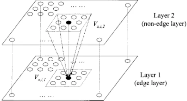
To enable the network to consider the pixel’s contextual information and identify whether or not each pixel is an edge point directly from an N⫻N image, the designed CHEFNN is made up of N⫻N⫻2 neurons, which can be conceived of as a two-layer Hopfield neural architecture. In the CHEFNN, the input is the original 2-D image and the output is an edge map. Each pixel of the image is assigned by two neurons arranged in a two layer, one atop another, as shown in Fig. 1, where each neuron represents one pos-sible label共edge point or not兲. Therefore, the output of the neurons with the same layer is an edge-based feature map. The architecture of the CHEFNN is shown in Fig. 1.
The CHEFNN is a two-layer neural network, extended from the one-layer 2-D Hopfield neural networks, where each neuron does not have self-feedback interconnection. Let Vx,i,kdenote the binary state of the (x,i)’th neuron in layer k (Vx,i,k⫽1 for excitation and Vx,i,k⫽0 for inhibi-tion兲 and Wx,i,k;y , j,zdenotes the interconnection weight
tween the neuron (x,i) in layer k and the neuron (y , j) in layer z. A neuron (x,i,k) in this network receives weighted inputs Wx,i,k;y , j,zVy , j,z from each neuron (y , j ,z) and a bias input Ix,i,kfrom outside. The total input to neuron (x,i,k) is computed as Netx,i,k⫽
兺
z⫽1 2兺
y⫽1 N兺
j⫽1 NWx,i,k;y , j,zVy , j,z⫹Ix,i,k, 共1兲
and the activation function in the network is defined by
Vx,i,kn⫹1⫽
再
1 共Netx,i,k⫺兲⬎0 Vx,i,kn 共Netx,i,k⫺兲⫽0
⫺1 (Netx,i,k⫺)⬍0
, 共2兲
whereis a threshold value. According to the update Eqs. 共1兲 and 共2兲, we can define the Lyapunov energy function of the two-layer Hopfield neural network as
E⫽⫺1 2k
兺
⫽1 2兺
z⫽1 2兺
x⫽1 N兺
y⫽1 N兺
i⫽1 N兺
j⫽1 N Vx,i,kWx,i,k;y , j,zVy , j,z ⫺兺
k⫽1 2兺
x⫽1 N兺
i⫽1 N Ix,i,kVx,i,k. 共3兲The network achieves a stable state when the energy of the Lyapunov function is minimized. The layers of the CHEFNN represent the state of each pixel which indicate if the pixel is an edge point. A neuron Vx,i,1in layer 1 in a firing state indicates that the pixel locate at (x,i) in the image is identified as an edge point, and a neuron Vy , j,2in layer 2 in a firing state indicates that the pixel located at (y , j) in the image is identified as a nonedge point.
To ensure that the CHEFNN has the ability to deal with contextual information in edge detection, the energy func-tion of CHEFNN must satisfy the following condifunc-tions.
First, in the nonedge layer, assume that a nonedge pixel (x,i) with Vx,i,2⫽1, and its surrounding nonedge pixels ( y , j ) within the neighborhood of (x,i)
⬘
with Vy , j,2⫽1 have the minimum Euclidean distance measure. Let gx,i and gy , jrepresent the gray levels of pixels (x,i) and (y , j), respectively. Then this condition can be characterized as follows:兺
x⫽1 N兺
y⫽1 (y , j)⫽(x,i) N兺
i⫽1 N兺
j⫽1 N dx,i;y , j⌽x,i p,q共y, j兲V x,i,2Vy , j,2, 共4兲where dx,i;y , j is the normalized difference between gx,iand gy , j, defined by dx,i;y , j⫽
冋
gx,i⫺gy , j max共G兲册
2 , 共5兲and⌽x,ip,q(y , j) is a function used to specify whether or not pixel (y , j) is located within a p⫻q window area centered at pixel (x,i). The function⌽x,i
p,q (y , j) is defined as ⌽x,i p,q共y, j兲⫽
兺
l⫽⫺q q ␦j,i⫹l兺
m⫽⫺p p ␦y ,x⫹m, 共6兲where␦i, j is the Kronecker delta function given by
␦i, j⫽
再
1 i⫽ j0 i⫽ j. 共7兲
With this definition⌽x,ip,q(y , j) will give a value 1 if ( y , j ) is located inside the window area, and 0 otherwise. In Eq.共4兲 Vx,i,2and Vy , j,2are used to restrict that the local gray-level differences are computed only for the pixels labeled by the nonedge layer.
Second, in the edge layer, if the labeling result of pixel (x,i) is the same as that of its neighboring pixels, then the energy function is decreased. Otherwise, the energy func-tion is increased. The similarity between each pixel’s label-ing result and its neighborlabel-ing pixels is computed as the following energy term:
兺
x⫽1 N兺
y⫽1 (y , j)⫽(x,i) N兺
i⫽1 N兺
j⫽1 N Vx,i,1Vy , j,2⌽x,i p,q共y, j兲, 共8兲In addition to the constraints mentioned above, the CHEFNN needs to satisfy the following two hard condi-tions to obtain a correct edge detection results:
1. Each pixel can be assigned by one and only one label 共edge or not兲:
兺
z⫽1
2
Vx,i,z⫽1. 共9兲
2. The sum of all classified pixels must be
兺
z⫽1 2兺
x⫽1 N兺
i⫽1 N Vx,i,z⫽N2. 共10兲From the preceding four constraints关Eqs. 共4兲, 共8兲, 共9兲, and 共10兲兴, the objective function of the network for edge detec-tion is obtained as E⫽A 2x
兺
⫽1 N兺
y⫽1 (y , j)⫽(x,i) N兺
i⫽1 N兺
j⫽1 Ndx,i;y , j⌽x,ip,q共y, j兲Vx,i,2Vy , j,2
⫹B 2x
兺
⫽1 N兺
y⫽1 (y , j)⫽(x,i) N兺
i⫽1 N兺
j⫽1 N Vx,i,1Vy , j,2⌽x,i p,q共y, j兲 ⫹C2兺
x⫽1 N兺
i⫽1 N兺
z⫽1 2兺
k⫽1 2 Vx,i,kVx,i,z ⫹D 2冉
z兺
⫽1 2兺
x⫽1 N兺
i⫽1 N Vx,i,z⫺N2冊
2 . 共11兲Note that the first two terms are soft constraints, which are used to improve the edge detection results共for example, to obtain a more complete and more connected edges兲. The
network should find a compromise between these soft con-straints. On the other hand, the last two terms are hard constraints. They are the basic requirements of the edge detection problem and cannot be violated. Thus, the net-work must completely satisfy these two hard constraints. Otherwise, the obtained results would not be accurate.
To avoid the difficulty of searching for proper values for the hard constraints, the competitive winner-take-all rule proposed by Chung et al.6is imposed in the CHEFNN for the updating of the neurons. Based on the winner-take-all rule for each pixel, one and only one of the neurons Vx,i,z, which receives the maximum input, would be regarded as the winner neuron and therefore its output would be set to 1. The other neurons Vx,i,z, for z⫽k associated with the same pixel are set to zero. Thus, the output function for Vx,i,k is given as
Vx,i,k⫽
再
1 if Vx,i,k⫽max兵Vx,i,1,Vx,i,2其
0 otherwise . 共12兲
The winner-take-all rule guarantees that no two neurons Vx,i,1 and Vx,i,2 fire simultaneously. The winner-take-all rule also ensures that all the pixels are classified. Due to these two properties, the last two terms共hard constraints兲 in Eq. 共11兲 can be completely removed. As a result, the ob-jection function of the CHEFNN may be modified as
E⫽
兺
k⫽1 2兺
z⫽1 2兺
x⫽1 N兺
y⫽1 (y , j)⫽(x,i) N兺
i⫽1 N兺
j⫽1 N冉
A 2dx,i;y , j␦z,2␦k,2 ⫹B2␦z,2␦k,1冊
⌽x,i p,q 共y, j兲Vx,i,kVy , j,z. 共13兲 Comparing the objection function of the CHEFNN in Eq. 共13兲 and the Lyapunov function Eq. 共3兲 of the two-layers Hopfield network, the synaptic interconnection strengths and the bias input of the network are obtained asWx,i,k;y , j,z⫽⫺
冉
A 2dx,i;y , j␦z,2␦k,2⫹ B 2␦z,2␦k,1冊
⌽x,i p,q共y, j兲 共14兲 and Ix,i,z⫽0, 共15兲respectively. Applying Eqs. 共14兲 and 共15兲 to Eq. 共1兲, the total input to neuron (x,i,k) is
Netx,i,k⫽⫺ 1 2z
兺
⫽1 2兺
y⫽1 (y , j)⫽(x,i) N兺
j⫽1 N 共Adx,i;y , j␦z,2␦k,2 ⫹B␦z,2␦k,1兲⌽x,i p,q共y, j兲V y , j,z. 共16兲From Eq.共16兲, we can see that due to the use of the com-petitive winner-take-all rule, the CHEFNN is not fully in-terconnected. The neurons located at the edge layer receive inputs from all the neurons in the edge layer and their as-sociated neighboring neurons in the nonedge layer. The neurons located at the nonedge layer receive inputs only
from the neurons at the nonedge layer. This property sig-nificantly reduces the complexity of the network, and thus, increases the network evolution speed.
3 Contextual-Constraint-Based Neural Cube Algorithm
The algorithm of the 3-D CHEFNN is summarized as fol-lows:
3.1 Input
The original image X, the neighborhood parameters p and q and the factors A and B.
3.2 Output
The stabilized neuron states of different layers representing the classified edge and nonedge feature map of the original images.
3.3 Algorithm
1. Arbitrarily assigns the initial neuron states to 2 classes.
2. Use Eq.共16兲 to calculate the total input of each neu-ron (x,i,k).
3. Apply the winner-take-all rule given in Eq. 共12兲 to obtain the new output states for each neuron. 4. Repeat steps 2 and 3 for all classes and count the
number of neurons whose state is changed during the updating. If there is a change, then go to step 2; oth-erwise, go to step 5.
5. Output the final states of neurons that indicate the edge detection results.
4 Convergence of the CHEFNN
In what follows, we prove that the energy function of the proposed CHEFNN is always decreased during network evolution. This implies that the network will converge to a stable state. Consider the energy function of the CHEFNN:
E⫽
兺
k⫽1 2兺
z⫽1 2兺
x⫽1 N兺
y⫽1 (y , j)⫽(x,i) N兺
i⫽1 N兺
j⫽1 N冉
A 2dx,i;y , j␦z,2␦k,2 ⫹B2␦z,2␦k,1冊
⌽x,i p,q 共y, j兲Vx,i,kVy , j,z. 共17兲 According to the architecture of CHEFNN, only the outputs of the neurons with the same layer and the outputs of the neighboring neurons with different layers may affect the classification result of pixel (m,n). Thus, the energy of Eq. 共17兲 can be separated into two terms, one related to the state of the neuron (m,n), E(m,n), and the other is irrel-evant to the state of the neuron (m,n), Eothers. Thus, the energy function of Eq.共17兲 can be rewritten as follows:E⫽E(m,n)⫹Eothers ⫽12
兺
k⫽1 2兺
z⫽1 2兺
y⫽1 (y , j)⫽(m,n) N兺
j⫽1 N 共Adm,n;y , j␦z,2␦k,2 ⫹B␦z,2␦k,1兲⌽m,n p,qV m,n,kVy , j,z ⫹1 2k兺
⫽1 2兺
z⫽1 2兺
x⫽1 x⫽m N兺
y⫽1 (y , j)⫽(m,n) N兺
i⫽1 i⫽n N兺
j⫽1 N 共Adx,i;y , j ⫻␦z,2␦k,2⫹B␦z,2␦k,1兲⌽x,i p,q Vx,i,kVy , j,z. 共18兲In Eq.共18兲, only the first term will be affected by the state of the neuron (m,n). Assume that the current iteration is to update the state of neuron (m,n). According to the winner-take-all learning rule, one and only one neuron is firing at position (x,i). Without loss of generality, it is assumed that the neuron (m,n,b) is the only active neuron at position (m,n) before updating, i.e., Vm,n,bold ⫽1 and Vm,n, jold ⫽0 ᭙i ⫽b. After updating, the neuron (m,n,a) is selected to be the winning node, i.e., Vm,n,anew ⫽1 and Vm,n, jnew ⫽0 ᭙i⫽a.
According to Eq.共16兲 and the winner-take-all rule, we obtain ⫺12
兺
z⫽1 2兺
y⫽1 (y , j)⫽(m,n) N兺
j⫽1 N共Adm,n;y , j␦z,2␦a,2
⫹B␦z,2␦a,1兲⌽m,n p,q共y, j兲V y , j,z ⫽maxk⫽1,2
冋
⫺ 1 2z兺
⫽1 2兺
y⫽1 (y , j)⫽(m,n) N兺
j⫽1 N 共Adm,n;y , j␦z,2␦k,2 ⫹B␦z,2␦k,1兲⌽m,n p,q共y, j兲V y , j,z册
, 共19兲which implies that
兺
z⫽1 2兺
y⫽1 (y , j)⫽(m,n) N兺
j⫽1 N共Adm,n;y , j␦z,2␦a,2
⫹B␦z,2␦a,1兲⌽m,n p,q共y, j兲V y , j,z ⬍
兺
z⫽1 2兺
y⫽1 (y , j)⫽(m,n) N兺
j⫽1 N 共Adm,n;y , j␦z,2␦b,2 ⫹B␦z,2␦b,1兲⌽m,n p,q共y, j兲V y , j,z. 共20兲Since the current updating of neuron states are associated with pixel (m,n), this updating will not change the value of Eothers. Thus the change of the energy values before and after network updating could be computed as
⌬E⫽Enew⫺Eold⫽E(m,n)new ⫺E(m,n)old ⫽1 2k
兺
⫽1 2兺
z⫽1 2兺
y⫽1 (y , j)⫽(m,n) N兺
j⫽1 N 共Adm,n;y , j␦z,2␦k,2 ⫹B␦z,2␦k,1兲⌽m,n p,q Vm,n,knew Vy , j,z ⫺12兺
k⫽1 2兺
z⫽1 2兺
y⫽1 (y , j)⫽(m,n) N兺
j⫽1 N 关Adm,n;y , j␦z,2␦k,2 ⫹B␦z,2␦k,1兴⌽m,n p,q Vm,n,kold Vy , j,z. 共21兲 According to the mentioned winner-take-all learning rule, we can see that Vm,n,anew ⫽1, Vm,n,inew ⫽0 ᭙i⫽a, and Vm,n,bold ⫽1, Vm,n,iold ⫽0 ᭙i⫽b. Thus, Eq. 共21兲 may be simplified as follows: ⌬E⫽12
冋
兺
z⫽1 2兺
y⫽1 (y , j)⫽(m,n) N兺
j⫽1 N共Adm,n;y , j␦z,2␦a,2
⫹B␦z,2␦a,1兲⌽m,n p,q 共y, j兲Vm,n,a new Vy , j,z ⫺
兺
z⫽1 2兺
y⫽1 (y , j)⫽(m,n) N兺
j⫽1 N 共Adm,n;y , j␦z,2␦b,2 ⫹B␦z,2␦b,1兲⌽m,n p,q共y, j兲V m,n,b old V y , j,z册
. 共22兲By replacing Vm,n,anew ⫽1 and Vm,n,bold ⫽1 in Eq. 共22兲, Eq. 共22兲 can be further simplified as follows:
⌬E⫽12
冋
兺
z⫽1 2兺
y⫽1 (y , j)⫽(m,n) N兺
j⫽1 N共Adm,n;y , j␦z,2␦a,2
⫹B␦z,2␦a,1兲⌽m,n p,q共y, j兲V y , j,z ⫺
兺
z⫽1 2兺
y⫽1 (y , j)⫽(m,n) N兺
j⫽1 N 共Adm,n;y , j␦z,2␦b,2 ⫹B␦z,2␦b,1兲⌽m,n p,q 共y, j兲Vy , j,z册
. 共23兲 The condition of Eq.共20兲 yields ⌬E⬍0. This implies that the energy change in the updating is negative. Therefore, the convergence of the CHEFNN is guaranteed.5 Experimental Results
To show that the proposed CHEFNN has a good capability of edge detection and noise immunity, three cases of dif-ferent modality medical images, including a computer-generated phantom image关Fig. 2共a兲兴, a skull-based CT im-age关Fig. 9共a兲 later in this section兴 and a knee-joint-based magnetic resonance 共MR兲 image 关Fig. 10共a兲 later in this section兴 were tested. All the cases used to evaluate the CCBHNC were collected from the National Cheng Kung University Hospital. The MR images were taken from the
Siemen’s Magnetom 63SPA, T2-weighted spin-echo se-quences, while the CT image is acquired from a GE 9800 CT scanner. The image sizes of CT and MR images are 256⫻256 pixels, with each pixel of 256 gray levels.
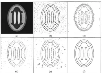
Figure 2共a兲 is a computer-generated phantom image, which was made up of seven overlapping ellipses. Each ellipse represents one structural area of tissue. From the periphery to the center, they were background共BKG, gray level⫽30), skin or fat 共S/F, gray level⫽120), gray matter 共GM, gray level⫽165), white matter 共WM, gray level ⫽75), and cerebrospinal fluid 共CSF, gray level⫽210), re-spectively. The gray levels for each tissue were set to a constant value, thus, the edge points can be easily obtained. The noise of the uniform distribution with the gray levels ranging from⫺K to K was also added to this simulation phantom to generate several noisy test images. The noise ranges were set to be 18, 20, 23, 25, and 30.
The proposed CHEFNN is compared with the Laplacian-based,7 Marr-Hildreth,1 Canny,8 and wavelet-based9 methods. In the evaluations, the most ap-propriate parameters共e.g., mask size N, local variance ␦, and threshold兲 for each method to gain the best edge detec-tion results in the original computer-generated phantom im-age are obtained by trial and error. These parameters will also be used in the methods in the subsequent test of noisy phantom images. The results using these methods for the noiseless image are shown in Figs. 2共b兲 to 2共f兲. From Figs. 2共b兲, 2共e兲, and 2共f兲, we can see that the Laplacian-based, Canny’s, and CHEFNN methods extract the edges correctly for the noiseless image. On the other hand, with the wavelet-based method, although it has the capability of edge detection, the result end up with disconnected edges, as shown in Fig. 2共d兲. Meanwhile, Fig. 2共c兲 shows that although the Marr-Hildreth method can extract complete edges it also results in redundant edges.
To evaluate noise robustness, these methods are also tested on noisy images of different noise levels. The results are shown in Figs. 3–7. Figures 3 and 4 are the results when the noise levels are small, with K⫽18 and 20, respec-tively. From Figs. 3 and 4 we can see that the CHEFNN
can obtain complete edges under a small level of noise, but other methods result in redundant edges. On the other hand, as the noise level increases, some redundant edges arise in the CHEFNN results, as illustrated in Figs. 5–7. Even so, the incurred amount of redundant edges with the CHEFNN is much less than with the other methods. These results imply that the CHEFNN has better noise immunity than other methods.
For quantitative evaluation, the detection error given by9 is used as the measurement:
Pe⫽ne n0
, 共24兲
where n0is the number of actual edge points, and neis the number of erroneous edge points. The edge detection per-formance for the Laplacian-based, Marr-Hildreth, Canny, wavelet-based, and CHEFNN methods are listed in Table 1 and are shown Fig. 8. From these results, we can easily see Fig. 2 (a) Original Phantom image, (b) result by the
Laplacian-based method, (c) result by the Marr-Hildreth method, (d) result by the wavelet-based method, (e) result by the Canny method, and (f) result by the proposed CHEFNN.
Fig. 3 (a) Phantom image with added noise (K⫽18), (b) result by the Laplacian-based method, (c) result by the Marr-Hildreth method, (d) result by the wavelet-based method, (e) result by the Canny method, and (f) result by the proposed CHEFNN.
Fig. 4 (a) Phantom image with added noise (K⫽20), (b) result by the Laplacian-based method, (c) result by the Marr-Hildreth method, (d) result by the wavelet-based method, (e) result by the Canny method, and (f) result by the proposed CHEFNN.
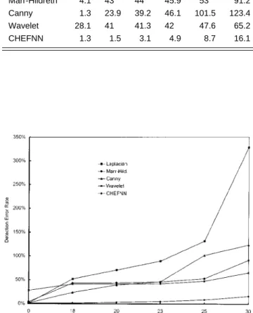
that although the wavelet-based methods lack accuracy in edge detection, they are relatively robust to noise. This can be easily observed by the flat curve in Fig. 8 showing the increase of the detection error rate from 28.1 to 65.2% as the noise level K increases from 0 to 30. On the other hand, the Laplacian-based and Canny methods perform well when the noise level K is equal to 0, with the detection error rates both equal to 1.3%. However, these two methods are highly noise sensitive. As the noise level increases, the detection error rate also increases dramatically to 328 and 123.4% for Laplacian-based and Canny methods, respec-tively. The Marr-Hildreth method has a relatively low de-tection error rate of 4.1% for noiseless image with K⫽0 and a relatively high error detection rate of 91.2% when K⫽30. In contrast to these methods, the proposed contextual-based CHEFNN obtains more correct edge re-sults for both noiseless and noisy images. The average de-tection error rate of CHEFNN is 1.3% for K⫽0, 1.5% for Fig. 5 (a) Phantom image with added noise (K⫽23), (b) result by the Laplacian-based method, (c) result by the Marr-Hildreth method, (d) result by the wavelet-based method, (e) result by the Canny method, and (f) result by the proposed CHEFNN.
Fig. 6 (a) Phantom image with added noise (K⫽25), (b) result by the Laplacian-based method, (c) result by the Marr-Hildreth method, (d) result by the wavelet-based method, (e) result by the Canny method, and (f) result by the proposed CHEFNN.
Fig. 7 (a) Phantom image with added noise (K⫽30), (b) result by the Laplacian-based method, (c) result by the Marr-Hildreth method, (d) result by the wavelet-based method, (e) result by the Canny method, and (f) result by the proposed CHEFNN.
Fig. 8 Detection error rates versus different noise levels. Table 1 The detection error rates for Laplacian-based,
Marr-Hildreth, Canny, wavelet, and the proposed CHEFNN methods us-ing the simulated phantom image withK⫽0 to 30.
Noise (%) Method 0 18 20 23 25 30 Laplacian 1.3 51.9 70.6 89.2 131.4 328.1 Marr-Hildreth 4.1 43 44 45.9 53 91.2 Canny 1.3 23.9 39.2 46.1 101.5 123.4 Wavelet 28.1 41 41.3 42 47.6 65.2 CHEFNN 1.3 1.5 3.1 4.9 8.7 16.1
K⫽18, 3.1% for K⫽20, 4.9% for K⫽23, 8.7% for K ⫽25, and 16.1% for the large noise level of K⫽30.
Figure 9共a兲 is a CT head image in which a number of tiny tissues exist. Figures 9共b兲 and 9共e兲 show the edge de-tection image using the Laplacian-based and wavelet-based methods, respectively. Obviously, the Laplacian-based and wavelet-based methods can not effectively outline the skull in the image. Thus, the edge detection results are poor. Figure 9共c兲 is the edge detection results of the Marr-Hildreth method. As we can see, there are double edges, many fragments, and little holes in the image. The results using Canny’s edge detector is illustrated in Fig. 9共d兲, which shows many unwanted details. Figure 9共f兲 is the edge detection results using CHEFNN. It clearly shows that more continuous edge were found when contextual infor-mation was used in the edge detection process. Thus, once again the proposed CHEFNN obtained clearer and more accurate edges in the image.
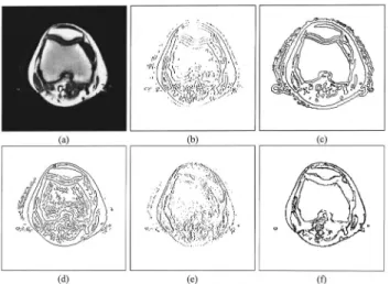
Figure 10共a兲 is an MR knee-joint-based transverse im-age. The edges of Fig. 10共a兲 obtained using the Laplacian-based method with threshold⫽5, N⫽7, and␦⫽1 and the Marr-Hildreth method with N⫽7 and ␦⫽1 are illustrated in Figs. 10共b兲 and 10共e兲, respectively. As we can see, there fragments and redundant edges exist in Laplacian-based and wavelet-based methods. Figure 10共c兲 illustrates the re-sult of the Marr-Hildreth method, from which we can see that edges extracted by the Marr-Hildreth method are con-siderably continued; however, the method also resulted in double edges. The result using the Canny edge detector is shown in Fig. 10共d兲. It is obvious from Fig. 10共d兲 that many unwanted details are also falsely detected by the Canny method as edges. The result obtained by CHEFNN is shown in Fig. 10共f兲 from which we can see that the bound-aries of the knee joint, articular, and patella were com-pletely and precisely detected.
6 Conclusion
In this paper, a modified Hopfield neural network architec-ture, the CHEFNN, is presented for edge detection of
medi-cal images. The CHEFNN extends the one-layer 2-D Hopfield network at the original image plane into a two-layer 3-D Hopfield network with the third dimension used for edge detection. With the extended 3-D architecture, the network is capable of including each pixel’s contextual in-formation into a pixels-labeling procedure. As a result, the effect of tiny details or noises can be effectively removed, and the drawback of disconnected fractions can also be overcome. The experimental results show that the CHEFNN produces more appropriate, continued, and intact edges in comparison with the Laplacian-based, Marr-Hildreth, Canny, and wavelet-based methods. In addition, using the competitive learning rule to update the neuron states prevents CHEFNN from satisfying strong con-straints. Thus, it enables the network to converge rapidly. In addition, the CHEFNN is a self-organized structure that is highly interconnected and can be implemented in a par-allel manner. It can also be easily designed for hardware devices to achieve high-speed implementation.
References
1. D. Marr and E. Hildreth, ‘‘Theory of edge detection,’’ Proc. R. Soc. London B207, 187–217共1980兲.
2. Y. Zhu and H. Yan, ‘‘Computerized tumor boundary detection using a Hopfield neural network,’’ IEEE Trans. Med. Imaging 16共1兲, 55–67 共1997兲.
3. S. W. Lu and J. Shen, ‘‘Artificial neural networks for boundary ex-traction,’’ in Proc. IEEE Int. Conf. on Systems, Man and Cybernetics, pp. 2270–2275共1996兲.
4. C. Y. Chang and P. C. Chung, ‘‘Using a three-dimensional Hopfield neural network for image segmentation,’’ in Proc. 1998 Conf. on Computer Vision, Graphics, and Image Processing, pp. 266–273, Taipei, Taiwan共1998兲.
5. J. J. Hopfield and D. W. Tank, ‘‘Neural computation of decisions in optimization problems,’’ Biol. Cybern. 52, 141–152共1985兲. 6. P. C. Chung, C. T. Tsai, E. L. Chen and Y. N. Sun, ‘‘Polygonal
approximation using a competitive Hopfield neural network,’’ Pattern Recogn. 27共11兲, 1505–1512 共1994兲.
7. J. S. Lim, ‘‘Two-dimensional signal and image processing,’’ Prentice-Hall, Englewood Cliffs, NJ共1989兲.
8. J. Canny, ‘‘A computational approach to edge detection,’’ IEEE Trans. Pattern. Anal. Mach. Intell. PAMI-8共6兲, 679–697 共1986兲. 9. T. Aydm, Y. Yemez, E. Anarim, and B. Sankur, ‘‘Multidirectional
and multoscal edge detection via M-band wavelet transform,’’ IEEE Trans. Image Process. 5共9兲, 1370–1377 共1996兲.
Fig. 9 (a) Original CT image; (b) result by the Laplacian-based method with threshold⫽5,N⫽7, and␦⫽1; (c) result by the Marr-Hildreth method (N⫽9,␦⫽1); (d) result by the Canny method; (e) result by the wavelet-based method; and (f) the result of CHEFNN (p⫽q⫽1,A⫽0.01,B⫽0.032).
Fig. 10 (a) Original MR knee-joint-based transverse image; (b) re-sult by the Laplacian-based method with threshold⫽5, N⫽7, and d⫽1; (c) result by the Marr-Hildreth method (N⫽9,d⫽1); (d) result by the Canny method; (e) result by the wavelet-based method; and (f) result by CHEFNN (p⫽q⫽1,A⫽0.01,B⫽0.03).
Chuan-Yu Chang received the BS degree in nautical technology from the National Taiwan Ocean University, Taiwan, in 1993, and the MS degree from the Department of Electrical Engineering, National Taiwan Ocean University, Taiwan, in 1995. Cur-rently, he is a PhD degree student with the Department of Electrical Engineering, Na-tional Cheng Kung University. His current research interests are neural networks, medical image processing, and pattern rec-ognition.
Pau-Choo Chung received the BS and the MS degrees in electrical engineering from National Cheng Kung University, Tainan, Taiwan, in 1981 and 1983, respectively, and the PhD degree in electrical engineer-ing from Texas Tech University, Lubbock, in 1991. From 1983 to 1986, she was with the Chung Shan Institute of Science and Technology, Taiwan. Since 1991, she has been with the Department of Electrical En-gineering, National Cheng Kung University, where she is currently a full professor. Her current research includes
neural networks, and their applications to medical image process-ing, medical image analysis, telemedicine, and video image analy-sis.