LECTURE 2

LECTURE 2

SAMPLED DATA ANALYSIS

LECTURE 2 - SAMPLED DATA ANALYSIS

• Sampling

• Shannon’s Sampling Theory

• Aliasing (Frequency folding)

• Zero-Order-Hold

WHAT IS SAMPLING?

• A continuous-time signal is replaced by a discrete sequence of

numbers that represents the signal value at certain (usually equally spaced) time intervals.

• A microprocessor based controller measures the physical process at discrete sample times and transmits new control signals at

discrete sampling times— sampled systems.

What is Sampling?

• A continuous-time signal is replaced by a discrete

sequence of numbers that represents the signal value at certain (usually equally spaced) time intervals.

• A microprocessor based controller measures the

physical process at discrete sample times and transmits new control signals at discrete sampling times—

sampled systems.

0 T 2T 3T 4T 5T

x(t)

x(t)

^Sample

x(kT) = x*(t)

x*

A sequence of number

x*(t) :

sampled signal

EFFECT OF SAMPLING

• “Sampling” creates certain effects that need to be understood.

• It is also important to understand whether it is possible, and if so how to reconstruct a continuous signal from its sampled data.

ME561 Lecture2- 3

Effect of Sampling

• “Sampling” creates certain effects that need to be understood.

• It is also important to understand whether it is

possible, and if so how to reconstruct a continuous signal from its sampled data.

0 T 2T 3T 4T 5T

x(t) reconstruct

x(t)

x(kT)

0 T 2T 3T 4T 5T

A SIMPLE LOOK AT ALIASING A Simple Look at Aliasing…

• Sampling frequency needs to be fast enough…

(Ex2_1)

0 0.5 1 1.5 2

-1.5 -1 -0.5 0 0.5 1 1.5

Time

Signal Amplitude

Orignal Signal Sampled Signal

-1 -0.5 0 0.5 1 1.5

Signal Amplitude

Original Signal Sampled Signal "o"

sampled Signal "x"

Twice as fast as the signal is fast enough?

WHAT IS SAMPLING

ME561 Lecture2- 5

What is Sampling? (revisit)

Mathematical representation of sampling

—the continuous-time signal is modulated with a train of (uniformly spaced) impulses

Taking periodic samples from a continuous-time signal x(t) to produce a sampled signal x(kT).

δ _T δ

k

t t kT

( ) = ( − )

=−∞

∑

∞

a train of impulses

CHARACTERISTICS OF IMPULSE FUNCTIONS Characteristics of Impulse Functions

• A time function with unitary area, with growing amplitude and shrinking duration.

• When it is multiplied to another time function

• Also known as the

Dirac Delta Function

– Paul Dirac (1902- 1984), English physicists

δ τ τ ( )

d

( )

t

t

=

z

−∞

¹

f t ( ) ( δ − t a dt ) = f a ( )

−∞

z

∞

The shifting property, true for all functions continuous at t=a.

L

δ ( )

t

= δ τ ( )

e^−sτ

⋅

d

τ =

−∞

z

∞

¹

( ) 0 when t t 0 & ( ) t dt 1 (Area = 1)

δ

^∞

δ

= ≠ ∫

−∞

=

SAMPLE OF A CONTINUOUS FUNCTION

ME561 Lecture2- 7

Sampling of a Continuous Function

* ( ) ( )

_T

( ) ( ) ( )

k

x t x t δ t

^∞

x t δ t kT

=−∞

= ⋅ = ∑ −

Sampled signal

Continuous-time

signal Impulse train

0 T 2T 3T 4T 5T

x*

0 T 2T 3T 4T 5T

x(t)

⊗

⊗

0 T 2T 3T 4T 5T

δ_T Impulse Train

( ) ( )

T

k k

t t kT

δ ^=∞ δ

=

∑

=−∞ −

• The sampling process can be interpreted as an amplitude

modulation (AM) process, where the C.T. signal x(t) is modulated by a carrier signal

δ

_T(t) with a carrier frequency

ω

_S ^{= 2}

π

/ T rad/sec, i.e.

LAPLACE TRANSFORM OF SAMPLED SIGNAL Laplace Transform of Sampled Signal

By definition

X *( ) s = x *( ) t = x *( ) ⋅ e d

^−s

−∞

z

∞

L τ

^τ

τ

* ( ) ( ) ( )

( ) ( ) ( )

s k

s skT

k k

X s x kT e d

x e kT d x kT e

τ

τ

τ δ τ τ

τ δ τ τ

∞ ∞ −

−∞ =−∞

∞ ∞ − ∞ −

=−∞ −∞ =−∞

 

=   −   ⋅

 

=   ⋅ −   =

∫ ∑

∑ ∫ ∑

Define z e =

^Ts

( ) *( ) ( )

^kTs

( )

^k

k k

X z X s

^∞

x kT e

^{− ∞}

x kT z

⁻

=−∞ =−∞

= = ∑ ⋅ = ∑ ⋅

The

“z-transform”

SIMPLE USAGE OF Z-TRANSFORM

• Given X(kT), find X(z)

• Given X(z), find X(kT)

X(z) = X*(s) = ∑

^∞

k=−∞

x(kT) ⋅ e

^−kTs

= ∑

^∞

k=−∞

x(kT) ⋅ Z

^−k

FREQUENCY INTERPRETATION OF SAMPLING Frequency Domain Interpretation of Sampling

Since δ

_T

(t) is periodic => can be represented by Fourier series

δ(t kT) C e

k

N

j T N t N

− = ⋅

=−∞

∞ F

HG I KJ

=−∞

∑ ∑

∞ ^2π

where C

_N

are the Fourier coefficients

C

_N

T e

^{j T N t}

dt

T

T t kT

k

=

⁻

⋅

=−∞

∑

∞ ⁻

^{F HG I KJ}

z

−

1

²

2

2 δ( )

π

T t e dt

T

j T N t T

=

T

⋅

⁻

F =

HG I KJ

z

−

1

²

1

2

2

δ( )

π

δ (t kT )

T e

k

j T N t N

− =

=−∞

∞

F

HG I KJ

=−∞

∑

¹

∑

∞ ^2π

ME561 Lecture2- 11

Frequency Domain Interpretation of Sampling(cont.)

Define the sampling frequency as (rad/sec)

ω _S = 2π T

X s x t x e d

e d

x e d x

T e d

T x e e d

T x e d

s

s

s s

j N s

s jN

x t kT

t kT e

k

k

j N N

N

N

S

S

S

*( ) *( ) *( )

( ) ( )

( ) ( )

( ) ( )

( )

= = ⋅

= ⋅

= L

NM O

QP ^{⋅ =} L

NM O

QP ^⋅

= ⋅ ⋅

⋅

−

−∞

∞

−

−∞

∞

−

−∞

∞ −

−∞

∞

−

−∞

∞

− −

−∞

∞

z z

z z

z z

−

−

=

=−∞

∞

=−∞

∞

=−∞

∞

=−∞

∞

=−∞

∞

∑

∑ ∑

∑

L

τ τ

τ

τ τ τ τ

τ τ

τ τ

τ

τ

τ τ

ω τ τ

ω τ

τ δ

δ

1

^{ω τ}

1 1

a f b g

b g

∑

X s

T X s jN _S

N

*( ) = ( − )

=−∞

∑

∞

1 ω

where X(s) is the Laplace

transform of x(t)

Frequency Domain Interpretation of Sampling(cont.)

ω X(jω)

1

ω₀ -ω₀

H(j

ω)

T x(t)

X(jω) x*(kT)

X*(jω) x_R(t)

X_R (jω)

ω₀

-ω₀ ω_S

-ω_S

1/T

X*(jω)

(ω_S – ω₀) ω

H(jω)

T

ω_C -ω_C

ω X_R(jω)

1

ω₀ -ω₀

X s

T X s jN _S

N

*( ) = ( − )

=−∞

∑

∞

1 ω

The frequency content is duplicated and created at multiple of The sampling frequency . There is a gain of 1/T due to sampling.

ω_S = 2π T

Ideal

Frequency Domain Interpretation of Sampling(cont.)

ω X(jω)

1

ω₀ -ω₀

H(j

ω)

T x(t)

X(jω) x*(kT)

X*(jω) x_R(t)

X_R (jω)

ω₀

-ω₀ ω_S

-ω_S

1/T

X*(jω)

(ω_S – ω₀) ω

H(jω)

T

ω_C -ω_C

ω X_R(jω)

1

ω₀ -ω₀

X s

T X s jN _S

N

*( ) = ( − )

=−∞

∑

∞

1 ω

The frequency content is duplicated and created at multiple of The sampling frequency . There is a gain of 1/T due to sampling.

ω_S = 2π T

Ideal

ME561 Lecture2- 13

Problem When ω

_S

^{< 2} ω

₀

ω X(jω)

1

ω₀

-ω₀ -2ω_S -ω_S 0 ω_S 2ω_S

××

2π/T

ω₀

-ω₀ ω_S

-ω_S

1/T

X*(jω)

(ω_S – ω₀) ω_S /2

ω_S > 2ω₀

1/T

X*(jω)

(ω_S – ω₀) ω_S -ω_S

-2ω_S 2ω_S

ω_S < 2ω₀

To reconstruct the (frequency content of the) original signal, a

necessary (but perhaps not sufficient) condition is that ω

_S

> 2ω

₀

SHANNON’S SAMPLING THEORY

• B.S. in EE & MATH, UMICH, 1932

• M.S. in EE, MIT, 1937

• “A Symbolic Analysis of Relay and Switching Circuits”

• The paper was a landmark in that it helped to

change digital circuit design from an art to a science

• Ph.D. in EE, MIT, 1940

• “An Algebra for Theoretical Genetics”

• Bell Labs & MIT

SAMPLING THEORY

ME561 Lecture2- 14

Shannon's Sampling Theorem

• (Sampling) Given a continuous-time band-limited signal x(t) with X(j ω)=0 for , x(t) can be uniquely determined by its samples x*(t) = x(kT), where k = 0,

±1, ±2, , if the sampling frequency ω

_S

> 2 ω

₀

Where

(Reconstruction) Given the sampled signal x*(t) = x(kT), x(t) can be reconstructed by processing x*(t) through an ideal low pass filter with cutoff frequency greater than ω

₀

and less than ( ω

_S

− ω

₀

) and a gain T in the pass band and 0 in the blocked region. The continuous-time signal can be computed from the sampled signal by the interpolation formula

ω ω >

₀

ω

_S

= 2π T

x t x kT

t kT t kT

S

k S

( ) ( )

sin ( )

( )

=

L

−

NM O

−

QP

=−∞

∑

∞

ω

ω 2

2

ME561 Lecture2- 14

Shannon's Sampling Theorem

• (Sampling) Given a continuous-time band-limited signal x(t) with X(jω)=0 for , x(t) can be uniquely determined by its samples x*(t) = x(kT), where k = 0,

±1, ±2, , if the sampling frequency ω_S > 2ω₀ Where

(Reconstruction) Given the sampled signal x*(t) = x(kT), x(t) can be reconstructed by processing x*(t) through an ideal low pass filter with cutoff frequency greater than ω₀ and less than (ω_S − ω₀) and a gain T in the pass band and 0 in the blocked region. The continuous-time signal can be computed from the sampled signal by the interpolation formula

ω ω> ₀

ω_S

= 2Tπ

x t x kT

t kT t kT

S

k S

( ) ( )

sin ( )

( )

=

L

−

NM O

−

QP

=−∞

∑∞

ω

ω 2

2

Proof of Shannon's Sampling Theorem

• The proof for the first half (sampling) of the sampling theorem has been sketched out in previous

discussions.

• We only need to figure out the “reconstruction” part

ω X(jω)

1

ω₀ -ω₀

H(j ω)

T x(t)

X(jω) x*(kT)

X*(jω) x_R(t)

X_R (jω)

ω₀

-ω₀ ω_S

-ω_S

1/T

X*(jω)

(ω_S – ω₀) ω

H(jω)

T

ω_C -ω_C

ω X_R(jω)

1

ω₀ -ω₀

ME561 Lecture2- 16

Proof of Shannon's Sampling Theorem

H(jω)

T

ω_C -ω_C

H j T

_S

S

( ω ) ω ω

= ω ω <

RS >

T ^{0 for for 2 2}

Ideal low pass filter (with a gain of T)

Sampled signal frequency

X j T X j

R

S S

( ) *( )

ω ω ω ω

= ⋅ ω ω <

RS >

T ^{0 for for 2 2}

If the ideal low pass filter is used, we have, between [- ω

_S

/2. ω

_S

/2], X

_R

(j ω)=X(jω).

• Reconstruction with an ideal low-pass filter H(j ω ^):

Perfect reconstr

( ) ( ) uction ! ! !

x t

R

x t

⇒ =

Proof of Shannon's Sampling Theorem (cont.)

2 2

( )

2 2

( ) 2

2 ( )

2

2

( ) 1 ( ) ( )

2 2

1 1

( ) ( )

( )

( )

sin 2

( ) (

( )

2

S S

S S

S S

S

S

j kT j t j t kT

k k

j t kT j t kT

k k

S S

S

k S

x t T x kT e e d T x kT e d

x kT e d x kT e

j t kT t kT

x kT x k

t kT

ω ω ω ω ω

ω ω

ω ω

ω ω

ω ω

ω ω

ω ω ω

ω ω

∞ ∞

− −

− −

=−∞ =−∞

∞ ∞ −

−

=−∞ − =−∞ −

∞

=−∞

 

= π ⋅   ⋅   ⋅ = π ⋅

= = ⋅

−

 − 

 

 

= − =

∑ ∑

∫ ∫

∑ ∫ ∑

∑ ^{) sinc}

^S

⁽ ₂ ⁾

k

T

ω

t kT

∞

=−∞

 − 

⋅    

∑

x t x t X j e d

T X j e d

R R

j t

j t

S S

( ) ( ) ( )

* ( )

= = ⋅

= ⋅ ⋅

−∞

∞

−

z z

1 2 1

2

²

2

π π

ω ω

ω ω

ω

ω

ω ω

sin( )

sinc( ) x

x =

Proof of Shannon's Sampling Theorem (cont.)

2 2 ( )

2 2

( ) 2

2 ( )

2

2

( ) 1 ( ) ( )

2 2

1 1

( ) ( )

( )

( )

sin 2

( ) (

( )

2

S S

S S

S S

S

S

j kT j t j t kT

k k

j t kT j t kT

k k

S S

S

k S

x t T x kT e e d T x kT e d

x kT e d x kT e

j t kT t kT

x kT x k

t kT

ω ω ω ω ω

ω ω

ω ω

ω ω

ω ω

ω ω

ω ω ω

ω ω

∞ ∞

− −

− −

=−∞ =−∞

∞ ∞ −

−

=−∞ − =−∞ −

∞

=−∞

 

= π ⋅  ⋅  ⋅ = π ⋅

= = ⋅

−

 − 

 

 

= − =

∑ ∑

∫ ∫

∑ ∫ ∑

∑

^{) sinc S (} ₂ ⁾

k

T ω t kT

∞

=−∞

 − 

⋅  

∑

x t x t X j e d

T X j e d

R R

j t

j t

S S

( ) ( ) ( )

* ( )

= = ⋅

= ⋅ ⋅

−∞

∞

−

z z

1 2 1

2

²

2

π π

ω ω

ω ω

ω

ω

ω ω

sin( )

sinc( ) x

x =

OBSERVATIONS

ME561 Lecture2- 18

Observations

The frequency ω

_N

⁼ ω

_S

/ 2 plays an important role in the sampling process. This frequency is called the Nyquist Frequency.

The reconstruction is only valid for signals that contains no frequency components higher than the Nyquist frequency ω

_N

⁼ ω

_S

^{/ 2.}

ω₀

-ω₀ ω_S

-ω_S

1/T

X*(jω)

(ω_S – ω₀) ω_S /2

ω_S > 2ω₀

1/T

X*(jω)

(ω_S – ω₀) ω_S -ω_S

-2ω_S 2ω_S

ω_S < 2ω₀

OBSERVATIONS Observations

• To achieve perfect reconstruction of the original signal at a specific time t*,

⇒ we will need all values of x(kT), past, present and future ! May be OK for some signal processing applications,

however, its not very practical for control applications …

( ( * )

( *) ) sinc

2

R S

k

t kT x

t k

x

^∞

T ω

=−∞

 − 

= ∑ ⋅    

ME561 Lecture2- 20

Ex2_2 Direct Implementation of SST

x t x kT

t kT t kT

S

k S

( ) ( )

sin ( )

( )

=

L

−

NM O

−

QP

=−∞

∑

∞

ω

ω 2

2

0 0.05 0.1 0.15 0.2 0.25 0.3 0.35 0.4 0.45 0.5

-0.2 0 0.2 0.4 0.6 0.8 1 1.2

Time (sec)

Amplitude Original Signal

Reconstructed Signal Sampled Signal

Why the lag?

sampled signal did not contain values before t = 0 and only has finite terms.

ALIASING Aliasing

• When the condition ω

_S

^{> 2} ω

₀

⁽ ω

_N

^> ω

₀

) is violated, the frequency content in the sampled data will be contaminated .

1/T

X*(jω)

(ω_S – ω₀) ω_S -ω_S

-2ω_S 2ω_S

ω_S < 2ω₀

The frequency components are copied, created and added

to the (true) low-frequency point.

ME561 Lecture2- 22

Aliasing (cont.)

X T X N

_s

*( ) ω = b g ¹ ∑

^∞N_=−∞

( ω − ω ) The frequency content of X*( ω) contains not only

that of X( ω), but also X(ω − ω

_S

), X( ω + ω

_S

), X( ω − 2ω

_S

), X( ω + 2ω

_S

), ...

Consider only positive frequencies, the spectrum at frequency ω actually includes (is the alias of) all the spectral components at ω, ω

_S

− ω, ω

_S

+ ω, 2ω

_S

− ω , 2ω

_S

+ ω, ... etc., where ω < ω

_N

^.

Mathematically

ω = |(ω + ω _N ) mod (ω _S ) − ω _N |

ALIASING

Aliasing (cont.)

• Graphical interpretation

• Mathematically,

ω = ( ω

₁

+ ω

_N

) mod( ω

_S

) − ω

_N

ω_N ω_S 3ω_N 2ω_S

ω_N

Actual Frequency

Sampled Frequency

ω

ω

(ω_S − ω ) (ω_S + ω ) (2ω_S − ω )

ME561 Lecture2- 24

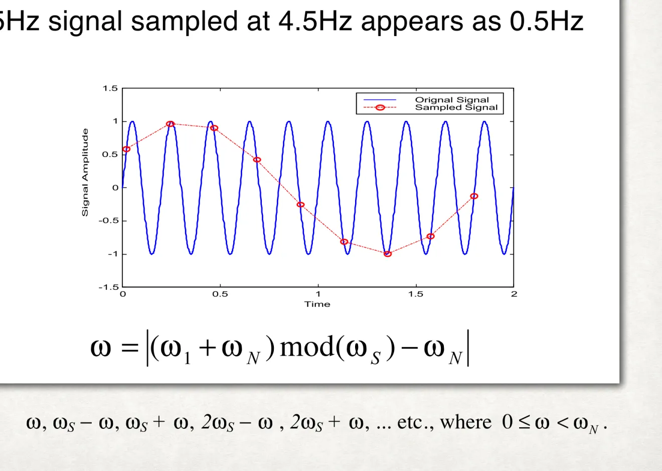
Ex2_1

• 5Hz signal sampled at 4.5Hz appears as 0.5Hz

0 0.5 1 1.5 2

-1.5 -1 -0.5 0 0.5 1 1.5

Time

Signal Amplitude

Orignal Signal Sampled Signal

ω = ( ω

₁

+ ω

_N

) mod( ω

_S

) − ω

_N

ME561 F^ALL 2001

H. Peng and George T.-C Chiu ©1994- 2001 SAMPLING – 9

0 0.1 0.2 0.3 0.4 0.5

-0.2 0 0.2 0.4 0.6 0.8 1 1.2

T i m e ( s e c )

Amplitude O r i g i n a l S i g n a l

R e c o n s t r u c t e d S i g n a l S a m p l e d S i g n a l

Figure 2.8 Signal Reconstruction

The result is illustrated in Figure 2.8. Note that the reconstructed signal is lagging behind the original signal. The reason is that the sampled signal did not contain values before t = 0 and only has finite terms. The interpolation formula is based on infinite series with both past and future samples available.

2 2 . . 3 3 A A l l i i a a s s i i n n g g

Shannon’s sampling theorem assumes that the continuous-time signal does not contain high frequency components outside the window (-ω0 , ω0 ) and the sampling time T is small enough that ω_N = π T > ω ₀ . When this assumption fails to hold, a phenomenon called aliasing will occur, which is illustrated in Figure 2.6.

When aliasing occurs, the original signal cannot be reconstructed even when the ideal low- pass filter H(jω) is used. From Eq. (2.5), if we treat the spectrum of X*(jω) as a function of ω, Eq.

(2.5) can be written as X *( )ω =

b g

¹ T

∑

_N^∞_=−∞ X (ω − Nω_s). Therefore, the frequency content of X*(ω) contains not only that of X(ω), but also X(ω − ωS), X(ω + ωS), X(ω − 2ωS), X(ω + 2ωS), ...

Since negative frequency components are used only for mathematics reasons, it is customary to consider only positive frequencies. The spectrum at frequency ω actually includes (is the alias of) all the spectral components in ω, ωS − ω, ωS + ω, 2ωS − ω , 2ωS + ω, ... etc., where 0 ≤ ω < ω_N . After sampling, a frequency thus cannot be distinguished from its alias. In general, a frequency component ω1 (ω1 > ωN ) appears as a low frequency component ω (ω < ωN ) after sampling, where

ω = (ω ω₁ + _N ) mod(ω _S ) − ω_N (2.9)

and all the frequencies are of the same units, rad/sec or Hz. Figure 2.9 shows a graph of the sampled frequency ω, in Eq. (2.9), versus the actual frequency.

Ex2_3 Example on Aliasing

• For a sampling time T = 0.2 seconds (5 Hz). Three sinusoidal signals (1Hz, 4Hz, and 6Hz) appear to be identical (as 1Hz, or rad/sec), since

ω

_S

− ω ^{= 5Hz} − ^{1Hz = 4Hz} ω

_S

⁺ ω = 5Hz + 1Hz = 6Hz

-1 -0.5 0 0.5

1

0 0.1 0.2 0.3 0.4 0.5 0.6 0.7 0.8 0.9 1

Time (sec)

Signal

6Hz

4Hz

ME561 Lecture2- 26

Ex2_4 Noise Aliasing

• Suppose you are trying to measure the acceleration of a vehicle, which has a limited bandwidth of 1.1Hz. If you select a sampling rate f

_S

= 11Hz (10 times faster than the system bandwidth), a noise of 700Hz (due to, say, the alternator) will appear as a 4Hz component.

ω = ( ω

₁

+ ω

_N

) mod( ω

_S

) − ω

_N

|(700+5.5)mod(11)-5.5| = 4.0

ANTI-ALIASING FILTERING Anti-Aliasing Filtering

• When a sampling rate ω

_S

is selected, it is implied that none of the frequency components larger than

ω

_N

, are of interest, since they cannot be reconstructed from the sampled data.

• Need to filter these components out to avoid contamination (aliasing, frequency folding).

• This anti-aliasing filter bandwidth is usually

selected to be higher than ω

_N

, but low enough to filter out major noise components.

Some important facts:

ME561 Lecture2- 28

Effects of Anti-Aliasing Filter

• The most significant effect due to anti-aliasing filter is the degradation of closed-loop phase margin.

Computer D/A

F(s) A/D

Anti-Aliasing Filter

G(s)

Plant

ZERO ORDER OF HOLD (ZOH) Zero Order Hold (ZOH)

• Zero order hold is a simple alternative (of SST) to

produce continuous-time signal from discrete-time

(sampled) signal.

SST - HARD TO IMPLEMENT

ME561 Lecture2- 30

SST—Hard To Implement

• SST

• Impulse response of the ideal low-pass filter:

x t x kT

t kT t kT

S

k S

( ) ( )

sin ( )

( )

=

L

−

NM O

−

QP

=−∞

∑

∞

ω

ω 2

2

-5 -4 -3 -2 -1 0 1 2 3 4 5

-0.4 -0.2 0 0.2 0.4 0.6 0.8 1

Normalized Time ( t / T )

Impulse Response

h t H j e d

T e d T e

jt

T

jt e e

t T t T

j t

j t T

T j t

T T

j t T j t T

( ) ( )

sin

= ⋅

= ⋅ = ⋅ = ⋅ −

=

F HG I KJ

−∞

∞

− −

−

z z

1 2

1

2 2 2

π

π π π

π π

π π

π π

π π

ω ω

ω

ω

ω ω

b g b g

e j

Non-causal—impossible to implement for time signals

ZOH ZOH

f t ( ) = f kT ( ) for kT ≤ < t ( k + 1 ) T Unit Impulse Response

X s x t t t T

s s e e s

R R

sT

sT

( ) = ( ) = ( ) − ( − )

= −

= −

−

−

L L 1 L 1

1 1 1

G

_ZOH

(jω)

^X*(jω)_x*(kT)

x_R(t) X_R (jω)

Time 0

1

Time 0

1

T

G s e

ZOH

s

sT

( ) = − 1

⁻

0 Time 1

T

FREQUENCY RESPONSE OF ZOH

ME561 Lecture2- 32

Frequency Response of ZOH

G j e

j

e e e

j T

T

T e

ZOH

j T j T j T j T j T

( )

sin

ω ω ω

ω ω

ω ω ω ω ω

= − = − =

F HG I KJ

_⋅

− − − −

1 2

2

2 2 2 1

a f

2

G s e

ZOH s

sT

( ) = −1 ⁻

( )

( )

sin 2 ( )

2

( ) sin 2

2

ZOH

ZOH

G j T T

T

G j T T

ω ω

ω

ω ω ω

 =



∠ = − + ∠



ME561 Lecture2- 33

Frequency Response of ZOH (cont.)

G_ZOH  T

0.637T

ω_N ω_S 2ω_S 3ω_S ω ω_S 2ω_S 3ω_S 0°

–180°

–360°

–540°

–720°

–900°

∠G_ZOH

ω_N ω_S 2ω_S 3ω_S 0

–20

– 40

– 60

G ZOH  dB

∠G ZOH

ω (rad/sec) 0°

–180°

–360°

–540°

–720°

–900°

ZOH V.S. IDEAL LOW PASS FILTER ZOH vs. Ideal Low Pass Filter

Hidden oscillation

ME561 Lecture2- 35

ZOH vs. FOH

[ ]

( ) ( ) t KT ( ) (( 1) ) for ( 1)

f t f kT f kT f k T kT t k T

T

= + − − − ≤ < +

ZOH FOH

Astrom and Wittenmark