適用於快取記憶體的封裝暨安置物件方法

(1)

國立臺灣大學電機資訊學院資訊工程學系博士論文

Department of Computer Science and Information Engineering College of Electrical Engineering & Computer Science

National Taiwan University Doctoral Dissertation

適用於快取記憶體的封裝暨安置物件方法 Cache Conscious Object Packing and Placement

林俊杰 Chun-Chieh Lin

指導教授：陳俊良博士 Advisor: Chuen-Liang Chen, Ph.D.

中華民國 98 年 1 月 January, 2009

(2)

(3)

(4)

(5)

致謝

99 年暮春、當我碩士畢業時，並沒有料想到十年之後，09 年初春，會再次地揮別母校與恩師陳俊良教授。追隨老師所學到的不僅僅是專業知識，還有許多人生的哲理和處事的態度。在這段漫長的求學過程中，看到老師辛勤的身影，弟子常常只能自覺汗顏。這篇論文與其說是我個人的研究成果，還不如說是老師與我的共同創作來得貼切。對於老師的感謝，無法全然一一道盡。

學長甘宗左博士在這幾年間給予我許多重要的協助，他一直鼓勵我要努力拼到畢業，長期以來在工作上也仰仗前輩的照顧，藉此機會也要表逹感謝。

這幾年花費了許多心力在學業上，因此要感謝內人思妤的支持。同時也要感謝我的父母多年來的栽培。此外岳父母、舍弟弟媳們，他們在戰線後方提供了許多後勤支援，也在此一齊感謝他們

2/1/2009, 俊杰於台北

(6)

摘要

快取記憶體在分層式記憶體架構中扮演加速存取動作的角色。程式與資料物件在記憶體中的排列順序是影響快取錯失率的重要原因之一。先賢們的研究都集中在找出適用於直接映射式快取記憶體的方法，其方法是把這些物件錯置排列至各個快取關連組。錯置排列的方法有助於減少衝突性錯失。然而某些系統的記憶區塊大到可以容納許多程式或資料物件，而且被讀進快取記憶體的最小單位是記憶區塊，而非物件，因此所有物件只得互搶快取記憶體內有限的空間。

本論文提出一套方法論，旨於利用調整物件在記憶體中排列的方法來改善快取記憶體的效率。這套方法包含兩項重點：探索物件的組織，以及針對各種快取架構產生專屬的物件排列法。探索物件組織的方法涵蓋了解構資料或程式的成份，以及產生物件存取活動的軌跡。此外本文亦特別提出一個適用於虛擬機器（例如爪哇虛擬機器）的探索技術，其著眼點是基於此類程式具有特殊的軟體架構。

本論文的重點是尋求產生適用於各類快取記憶體的物件排列之法。前提是假定物件的尺寸小於記憶區塊。這意味著賦予物件地址編號必須統合兩項動作，一則是用於快取關連組錯置物件法，二則是將物件合併到記憶體區塊。本論文提出的辦法是藉由存取活動的軌跡來建立物件關連模型。在發展的過程中，文本分析了物件關連模型、快取架構、及快取錯失之間的因果關係。然而這些因果關係實際上十分困難而無法算出最佳解。因此本文也提出頗具實用性的技術，用以產生適用於不同快取架構的物件排列法。本論文亦實作了相當繁複的實驗來驗證所提出來的方法。實驗的結果頗具有說服力，可以支持本文提出的技術的有效性。

關鍵字：快取記憶體;記憶體最佳化;程式碼排列;資料排列;虛擬機器

(7)

Abstract

The cache provides acceleration in access through the memory hierarchy. The order of arranging code and data objects in the main memory is an important factor that affects cache miss rates. Prior related researches focus on arranging objects interleaved between cache sets for the direct mapped cache. Interleaving the address of each items helps to resolve conflict misses. However, there are computer systems that a memory block can be large to collect a number of code and data objects, and the unit to be loaded to the cache is a memory block, not an object. Therefore, objects contend spaces within cache blocks as well.

This dissertation provides a methodology for optimizing cache memory utilization of applications in various fields by arranging their relocatable objects within the main memory. The methodology includes the exploration of object space and generation of object layouts for all kinds of cache organization. The object space exploration involves techniques in inspecting the data and program integrant and acquiring the profile of objects accesses. The exploration also contains a technique particular for the virtual machine, e.g., the Java virtual machine, because of its unique program structure.

Generating object layout adapted for cache memory is the keystone in this dissertation. The presumption is that objects are smaller than a memory block. That means assigning addresses to objects must incorporate two movements into one. The first is interleaving objects to cache sets. The second is gathering these objects to fit one cache block. Our study suggests creating the object affinity model by profile

(8)

information. This study analyzes the relationship between the object affinity model, cache configurations, and cache misses. The packing and placement problem turns to be hard to find an optimal solution. Thereafter, this study proposes practical techniques of generating object layouts for different cache organizations. This dissertation also includes experiments to evaluate the proposed techniques. The experiments provide convincible results and support the effectiveness of the proposed approaches.

Keywords: cache memory; memory optimization; code layout; data layout; virtual machine

(9)

List of Figures

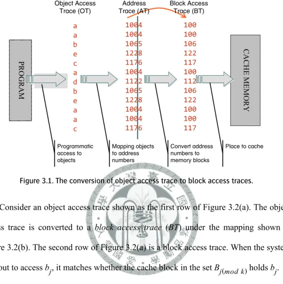
Figure 1.1. The framework of manipulating packing and placement for cache memory in different problem domains... 6 Figure 2.1 The memory hierarchy. ... 9 Figure 2.2. Execute programs stored in a NAND flash memory by using a shadow RAM... 16 Figure 2.3. Execute programs stored in a NAND flash memory by using a cache... 17 Figure 3.1. The conversion of object access trace to block access traces. ... 33 Figure 3.2. (a) An example of object access trace, block access trace, and compressed block

access trace in three rows. (b) A legal packing mapping that injects six objects to three memory blocks. ... 33 Figure 3.3 (a) The adjacent matrix. (b) The object access graph. (c) Group the original object trace graph into partitions... 37 Figure 3.4. Define the type of edges in the access graph. ... 40 Figure 3.5. (a) An example of object access trace, block access trace, block access sub-traces,

and compressed block access sub-traces. (b) A legal f

pp injects eight objects to four memory blocks... 43 Figure 3.6. The components of an object access graph for the direct mapped cache... 44 Figure 3.7. (a) An example of object access trace, block access trace, and compressed block

access trace in three rows. (b) A legal packing mapping that injects six objects to three memory blocks. ... 49 Figure 3.8. Choose the least used elements by the OPT replacement. ... 51 Figure 3.9. Compare the two locality sets along the object access trace... 52 Figure 3.10. The object locality set hold by the cache contributes lengths to the edges of the objects access graph. ... 52 Figure 3.11. Using Degree-2 and Degree-3 trace information to find the closest objects to

(13)

Figure 4.1. A partitioned graph satisfies MIN k-PARTITION. The symbols wi and pi denote

edge lengths. ... 62

Figure 4.2. A sample graph transformed from Figure 4.1. ... 63

Figure 4.3. The pseudo code of the partitioning algorithm ... 66

Figure 4.4. The pseudo code of distributing blocks to sets... 69

Figure 4.5. The partition result after the first pass. The gray edges connect the access trace graph before partitioning. The two shadowed blocks are the generated partitions. .... 73

Figure 4.6. The partition result after the second pass. ... 73

Figure 5.1. A program fragment to be rearranged. ... 79

Figure 5.2. Two layouts of program statements. ... 79

Figure 5.3. The basic blocks involved in a function call. ... 81

Figure 5.4. The example illustrates transformation between the ordinary and the variant basic block. The left pseudo code is what the CFG represents for... 84

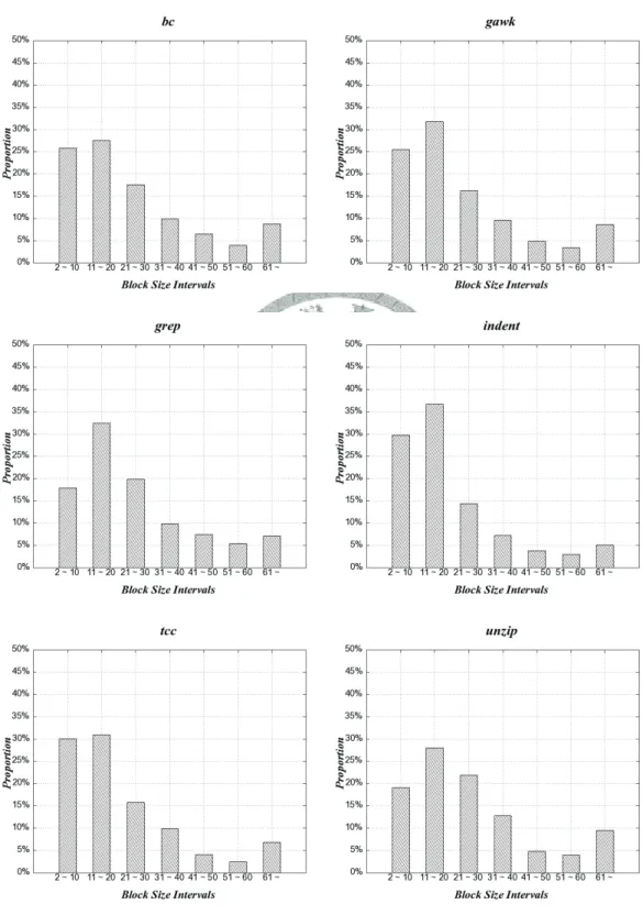
Figure 5.5. Distribution of different sizes of basic blocks within each benchmark programs. ... 88

Figure 5.6. The contributions of (non-zero length) edges in object access graphs of benchmark programs. The x-axis denotes number of edges arranged by the length in descending order, from left to right. The y-axis represents the sum of edge length from the left-most edge to the current position. The x-axis is cut-off at 30% since 30% of edges contribute more than 90% of overall edge lengths. ... 90

Figure 5.7. The number of vertexes connected by the non-zero length edges in the object access graphs. The meaning of the x-axis is identical to the previous chart. The y-axis represents the sum of connected vertexes of the edges from the left-most end to the current position. ... 91

Figure 5.8. The chart shows the ratio between the sum of edge length and the number of connected vertexes of benchmark programs. The meaning of x-axis is identical to the y-axis of Figure 5.6, and the meaning of y-axis is identical to the y-axis of Figure 5.7.92 Figure 5.9 Pseudo code of KVM interpreter... 97

(14)

Figure 5.10 Control flow graph of the interpreter ... 97

Figure 5.11. The organization of the interpreter at assembly level ... 98

Figure 5.12 Distribution of Bytecode Handler Size (compiled by gcc-3.4.3) ... 99

Figure 5.13 The CFG of the simplified interpreter... 101

Figure 5.14. An ICFG example. The number inside the circle represents the size of the handler. ... 101

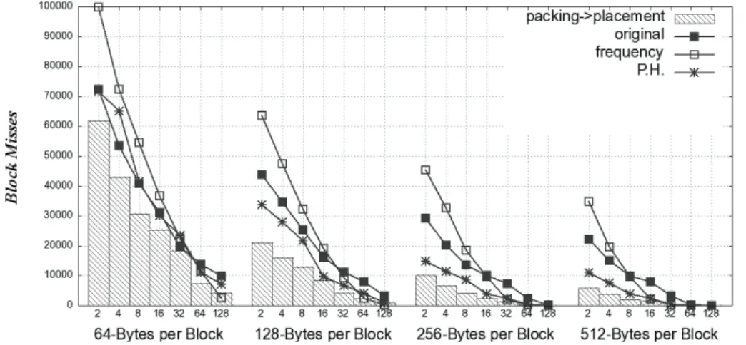
Figure 6.1. Block misses of bc by the four packing and placement implementation. The chart juxtaposes the results from those working on different cache configurations; differ by block size and number of sets (x-axis)... 118

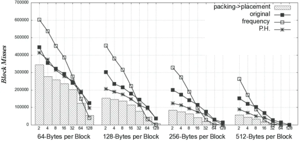
Figure 6.2. Block misses of gawk by the four packing and placement implementation, from experiments working on caches differ by blocks size and sets. ... 118

Figure 6.3. Block misses of grep by the four packing and placement implementations, from experiments working on caches differ by blocks size and sets ... 118

Figure 6.4. Block misses of indent by the four packing and placement implementations, from experiments working on caches differ by blocks size and sets ... 119

Figure 6.5. Block misses of the tcc by the four packing and placement implementations, from experiments working on caches differ by blocks size and sets ... 119

Figure 6.6. Block misses of unzip by the four packing and placement implementation, from experiments working on caches differ by blocks size and sets ... 119

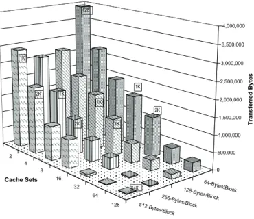
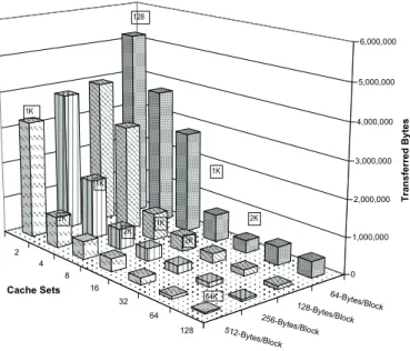
Figure 6.7. An overall observation, in both the respect of block size and cache set counts, of the block misses caused by the layout of bc by the packing first and placement next approach. The label aside the column indicates the total size of the cache of the given experimental condition. ... 120

Figure 6.8. An overall observation, in both the respect of block size and cache set counts, of the block misses caused by the layout of gawk by the packing first and placement next approach... 120

(15)

Figure 6.9. An overall observation, in both the respect of block size and cache set counts, of the block misses caused by the layout of grep by the packing first and placement next approach... 121 Figure 6.10. An overall observation, in both the respect of block size and cache set counts, of

the block misses caused by the layout of indent by the packing first and placement next approach... 121 Figure 6.11. An overall observation, in both the respect of block size and cache set counts, of

the block misses caused by the layout of tcc by the packing first and placement next approach... 122 Figure 6.12. An overall observation, in both the respect of block size and cache set counts, of

the block misses caused by the layout of unzip by the packing first and placement next approach... 122 Figure 6.13. Estimate the amount of data read from main memory by all cache misses (bc).

... 123 Figure 6.14. Estimate the amount of data read from main memory by all cache misses

(gawk)... 123 Figure 6.15. Estimate the amount of data read from main memory by all cache misses (grep).

(indent)... 124 Figure 6.17. Estimate the amount of data read from main memory by all cache misses (tcc).

(unzip). ... 125 Figure 6.19. Compare layouts of bc by packing and placement with other approaches. .... 126 Figure 6.20. Compare layouts of gawk by packing and placement with other approaches.126 Figure 6.21. Compare layouts of grep by packing and placement with other approaches.. 126

(16)

Figure 6.22. Compare layouts of indent by packing and placement with other approaches.

... 127 Figure 6.23. Compare layouts of tcc by packing and placement with other approaches. ... 127 Figure 6.24. Compare layouts of unzip by packing and placement with other approaches.

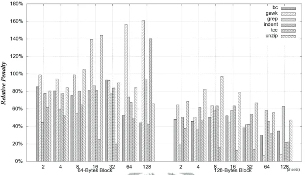
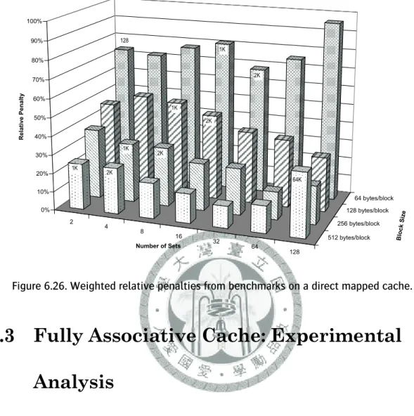
... 127 Figure 6.25. Relative penalties of all benchmarks for the cases that block size are 64 and 128

bytes. ... 128 Figure 6.26. Weighted relative penalties from benchmarks on a direct mapped cache... 129 Figure 6.27. The miss counts caused by all kinds of layout of bc working on a fully

associative cache with FIFO replacement. ... 132 Figure 6.28. The miss counts caused by all kinds of layout of bc working on a fully

associative cache with LRU replacement. ... 133 Figure 6.29. The miss counts caused by all kinds of layout of gawk working on a fully

associative cache with FIFO replacement. ... 133 Figure 6.30. The miss counts caused by all kinds of layout of gawk working on a fully

associative cache with LRU replacement. ... 133 Figure 6.31. The miss counts caused by all kinds of layout of grep working on a fully

associative cache with FIFO replacement. ... 134 Figure 6.32. The miss counts caused by all kinds of layout of grep working on a fully

associative cache with LRU replacement. ... 134 Figure 6.33. The miss counts caused by all kinds of layout of indent working on a fully

associative cache with FIFO replacement. ... 134 Figure 6.34. The miss counts caused by all kinds of layout of indent working on a fully

associative cache with LRU replacement. ... 135 Figure 6.35. The miss counts caused by all kinds of layout of tcc working on a fully

associative cache with FIFO replacement. ... 135 Figure 6.36. The miss counts caused by all kinds of layout of tcc working on a fully

associative cache with LRU replacement. ... 135

(17)

Figure 6.37. The miss counts caused by all kinds of layout of unzip working on a fully associative cache with FIFO replacement. ... 136 Figure 6.38. The miss counts caused by all kinds of layout of unzip working on a fully

associative cache with LRU replacement. ... 136 Figure 6.39. Relative penalties of all benchmarks for the cases that block size are 64 and 128

bytes on a fully associative cache with FIFO replacement. ... 136 Figure 6.40. Relative penalties of all benchmarks for the cases that block size are 64 and 128

bytes on a fully associative cache with LRU replacement... 137 Figure 6.41. Weighted relative penalties from benchmarks on a fully associative cache with FIFO replacement. ... 138 Figure 6.42. Weighted relative penalties from benchmarks on a fully associative cache with LRU replacement. ... 139 Figure 6.43. Weighted relative penalties from benchmarks on a set associative cache. .... 148 Figure 6.44. Perform packing and placement on a subset of basic blocks. The percentage of

each column stands for the threshold for screening basic blocks by adjacent edges’

lengths (bc)... 151 Figure 6.45. Perform packing and placement on a subset of basic blocks. The percentage of

lengths (gawk). ... 151 Figure 6.46. Perform packing and placement on a subset of basic blocks. The percentage of

lengths (grep). ... 151 Figure 6.47. Perform packing and placement on a subset of basic blocks. The percentage of

lengths (indent). ... 152 Figure 6.48. Perform packing and placement on a subset of basic blocks. The percentage of

lengths (tcc)... 152

(18)

Figure 6.49. Perform packing and placement on a subset of basic blocks. The percentage of each column stands for the threshold for screening basic blocks by adjacent edges’

lengths (unzip)... 153 Figure 6.50. Weighted relative penalties of all threshold levels for different cache

organizations. ... 153 Figure 6.51. Pack subsets of basic blocks for the fully associative cache, and calculate the

relative penalties of the packed layout and the original layout. (bc)... 155 Figure 6.52. Pack subsets of basic blocks for the fully associative cache, and calculate the

relative penalties of the packed layout and the original layout. (gawk) ... 156 Figure 6.53. Pack subsets of basic blocks for the fully associative cache, and calculate the

relative penalties of the packed layout and the original layout. (grep) ... 156 Figure 6.54. Pack subsets of basic blocks for the fully associative cache, and calculate the

relative penalties of the packed layout and the original layout. (indent)... 156 Figure 6.55. Pack subsets of basic blocks for the fully associative cache, and calculate the

relative penalties of the packed layout and the original layout. (tcc)... 157 Figure 6.56. Pack subsets of basic blocks for the fully associative cache, and calculate the

relative penalties of the packed layout and the original layout. (unzip) ... 157 Figure 6.57. Weighted relative penalties of all threshold levels for different cache

organizations. ... 157 Figure 6.58 Hierarchy of simulation environment ... 159 Figure 6.59. Entities in the refinement process... 160 Figure 6.60. The chart of the experimental relative penalty. Each line is an experiment

works on a given memory block size. The x-axis is the size of the cache memory ( number_of_blocks * block_size ). ... 165 Figure 6.61. The chart of the experimental relative penalty. The x-axis is the number of

cache blocks. ... 165

(19)

List of Tables

Table 2.1. Typical combinations of NAND flash blocks and pages... 16

Table 5.1. A briefing of benchmark programs... 87

Table 5.2. The basic block statistics of benchmark programs... 87

Table 5.3. The basic block statistics of object access traces ... 87

Table 6.1. Cache misses caused by layouts of bc program and its relative penalties. ... 142

Table 6.2. Cache misses caused by layouts of gawk program and its relative penalties. ... 143

Table 6.3. Cache misses caused by layouts of grep program and its relative penalties... 144

Table 6.4. Cache misses caused by layouts of indent program and its relative penalties. . 145

Table 6.5. Cache misses caused by layouts of tcc program and its relative penalties... 146

Table 6.6. Cache misses caused by layouts of unzip program and its relative penalties.... 147

Table 6.7. Sub-graph size and computation costs by different levels of threshold... 150

Table 6.8. Sub-graph size and computation costs by different levels of threshold... 155

Table 6.9. Experimental cache miss counts. Data of 21 to 32 pages are omitted due to being less relevant... 164

Table 6.10. Average accessed page of each bytecode handler and the bottom position of the curves of relative penalty... 166

(20)

(21)

Chapter 1

Introduction

1.1 Motivation

The memory hierarchy of a computer system breaks into levels by speed and capacity. A higher-level memory has shorter access time, but the unit cost of capacity is higher. On the contrary, a lower-level memory offers large capacity but suffers slower access time. Cache memory is a compromising approach for accelerating access to a large amount of data. A cache is a temporary storage area resides in the faster memory.

It constantly holds frequent-accessed items duplicated from the slower memory or secondary storage. Therefore, access operations to the slower memory can be replaced with fast accesses to the cache memory once it holds desired data items. This is how cache memory helps to increase the system performance. There are several ways to improve the cache performance. One aspect is to increase the cache hits (or reduce the cache misses, vice versa). If the cache memory can hold more active data items, one can decrease the accesses to the slower memory.

There are several factors affect cache misses. One among those is the arrangement of code/data items, or say object, in the memory space. The term “object” can be a program variable in the main memory or basic blocks in programs. The activities of

(22)

accessing objects are actually manipulating contents in the cache memory. The activities comprise a series of invalidating cache blocks and loading memory blocks, and cause consecutive cache hits and misses.

The address number is the key parameter of the cache mapping function. It determines the placeholder in the cache memory for an object associated with a given address. The address translation consists of arithmetical steps. The activities of accessing objects can be considered as manipulating contents in the cache memory. A cache memory accesses main memory by blocks, and the address space is segmented into blocks. As a result, the access activities comprise a series of invalidating cache blocks and loading memory blocks, and cause consecutive cache hits and misses.

Besides, the objects belonging to the same set contend for the same cache block.

Summarizing these factors, the assignment of address numbers to objects indirectly affects the activity of accesses to the cache memory and the occurrences of cache misses. This is the origin of the object placement problem.

The problem is not a new topic in the study of compilers. At the code generation stage of a compiler, it has to assign basic blocks in a control flow graph to the linear address space. That is to render instructions following a certain arrangement. The arrangement of instruction codes may incorporate with the optimization process for memory hierarchy (as discussed in [1]). Furthermore, this problem can be applied to arrange general data items in the memory or storages beyond the optimizing compilers.

Typical object placement methods consider that an object is roughly the same size as one cache block and memory block, e.g., Gloy et al. [2]. That implies a memory

(23)

block can hold one object. This is true in many real applications. However, there are also real applications that a memory block is bigger than an object. Therefore, a memory block can gather a number of objects. The nature of some architectures leads to large memory blocks and cache blocks. This is significant to embedded systems, since a processor or a program often manipulates memory devices with large storage blocks directly. For example, a modern embedded processor may have built-in NAND flash memory interface, and the program can interact the chips directly. The unit of a read operation of a NAND flash memory is a page with 4096-byte in size. In this case, one flash page can gather several data objects. The assignment of data objects to flash pages can affect the number of the accesses to the flash memory by a program. This causes one of the performance issues for embedded systems.

Properly grouping objects to memory blocks can help to gather more information being used into cache blocks, and reduce cache misses eventually. Consider a simple example that accesses objects (a, b, c) in the following order {a,c,a,c,b}. It is easy to find that packing (a,b) into one memory block can cause more misses than packing (a,c) together. The policy is to figure out closely appeared objects and packs them together into a group. Eventually, this policy acts like a predictor that helps to load the objects being used in advance. When object a is loaded into the cache for the first access activity, object c is loaded spontaneously, because both of them are located in the same memory block. Therefore, the next access activity can reach object c immediately without any miss.

These preconditions make assigning addresses to objects a complicated problem, and it is not covered by other pioneers’ works. Our study suggests the address

(24)

assignment task must incorporate two movements into one. The first is interleaving objects between cache sets. The second is gathering objects to fit one memory block.

We term the first movement “placement” and the second one “packing”. This dissertation presents a systematic approach in dealing with this problem. Our approach uses profile information as a guide to arrange objects in the memory spaces. The profile information is used to create object access model. The relations between the object access model, cache configurations, and the origin of cache misses are investigated.

Finally, our research proposes a technique to generate object layout that can be expected to improve cache performance.

1.2 Usefulness

Our approach is good for the real application that needs to gather objects to one block. Consider the scenario of interfacing to a file system. A file system segments a file and save them to the storage units, or say blocks, clusters, or chunks in different terms. For instance, the Ext2 file system, widely used in Linux ([3]), supports block size of 1024, 2048, or 4096 bytes. That means a block can hold some records of the file. If all the records are randomly arranged, it leads the possibilities of accessing each block distribute uniformly. That means the process is apt to access blocks absent in the disk cache, and the benefit of using the disk cache is reduced. However, if the record arrangement follows our approach, the locality of accessing blocks would be improved.

Precisely speaking, the process is likely to access blocks reside in the disk cache within a certain duration.

(25)

NAND flash memory plays multiple roles to a computer system. It can be used as a secondary storage device, as well as a non-volatile memory that directly connected to a CPU. Because of the hardware characteristics, demand paging is a common technique used to interface NAND flash [4]. Therefore, there are challenges in using NAND flash in an embedded system. Using NAND flash as code memory is called execute-in-place (XIP), and we shall discuss about XIP in the next section. On the other hand, in either the respect of NAND flash page or block, a storage unit is large enough to hold several data objects together. Naturally, storing data objects in NAND flash also faces the packing and placement problem.

(26)

1.3 Scope and Organization

Capture trace information of generic

data objects Classify data objects

from the problem domain

Using packing and placement techniques to generate object layout

For Fully Associative Cache

For Direct Mapped Cache

For Set Associative Cache

Arrange data objects in the memory

Use profiler to capture trace information of

code objects Classify code objects

in programs using a compiler

Generate a refined program with give code object layout

Capture indirect trace information of the

executed Java programs Analysis the program

structure of a Java virtual machine

Java Programs

Generate a refined Java virtual machine

Pre-Processing Stage Object Class-dependentProcessing Stage Object Class-independentPost-Processing Stage Object Class-dependent

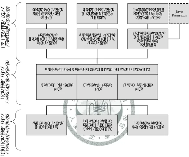
Figure 1.1. The framework of manipulating packing and placement for cache memory in different problem domains.

The main purpose of this dissertation focuses on modeling the object packing and placement for the three major kinds of cache organization. In addition, the treatment to different field of applications is also included in this research. Figure 1.1 illustrates the entire framework associated with the object packing and placement process.

The top part in the framework prepares parameters that are used by the packing and placement algorithms. The mission of the top part is to mark out the scope and

(27)

usage of objects for profile information. The techniques used to collect the profile information vary by the field of application. Dealing with generic data items can be straightforward. Technique for program code arrangement may involve with the study in compilers. The arrangement of a virtual machine, like Java Virtual Machine, can be a unique class. Developing the technique requires insight into the design of a virtual machine. Therefore, it deserves a detailed discussion in this dissertation. All these relevant techniques are presented in Chapter 5.

The block in the middle of the framework can be regarded as a black box. The inputs of the black box are parameters describes object characteristics and profile information. The mission of the black box is generating object layout for a specific type of cache memory. The design of the black box is the core of our research. To characterizing the nature of the problem, this dissertation formulates the problem model in Chapter 3. A thorough understanding of the problem model helps us to propose solutions of packing and placement problems, in Chapter 4, that practical enough to be utilized in real compilers or applications.

Chapter 6 has a series of experiment that utilize the proposed techniques to face real application. The experiments demonstrate the proposed techniques should work fine with program code arrangement on different cache organizations.

Before digging into the major article of this dissertation, Chapter 2 shall widely survey topics related with our research and explain why the pioneers’ works did not cover our research subject.

(28)

(29)

Chapter 2

Background

2.1 Memory Hierarchy

A computer system may require a large memory for storing program and data. Not all of them are accessed by the computer system simultaneously at any moment because of the principle of locality ([5]). A computational process typically accesses program codes and data items in the memory in a clustered manner. The locality behavior has two extents. Temporal locality models the access activties along time axis. A temporal locality set of objects are likely to be referenced occasionally within a given period.

Spatial locality means that a process is likely to access objects in several geometric neighborhoods in storage devices during the whole lifetime.

CPU

Level-1 Cache Level-2 Cache

Main Memory

Hard Drive / CDROM

within the chip

Figure 2.1 The memory hierarchy.

(30)

The memory hierarchy is a compromised approach to manage massive code and data objects in an efficient way. As shown in Figure 2.1, memory devices are stacked by access speed. The fastest memory is attached to the CPU directly, such as an on-chip static RAM. The slowest memory device is placed in the bottom layer, such as hard drive or CDROM. Objects are loaded to the upper layer before being used. Because a small portion of objects will be used, the capacity of the upper layer is usually smaller than the lower layer. The concept can be applied to many places in a computer system, such as the CPU cache in a processor, TLB to paged memory management, and virtual memory in an operating system [6][7]. Technically speaking, the system design policy can freely devise the scheme of exchanging objects between the upper and lower memories. However, cache memory plays an important role for this purpose.

2.1.1 Cache Organization

Cache memory is a mechanism dedicated for using a piece of small and fast memory to manipulated data contents stored in a large and slow main memory. In respect of functionality, it is a set of protocol to manage buffers in the memory. A cache memory consists of cache blocks (cache lines), thereby dividing the main memory into blocks. When a processor is about to access raw data in the main memory, raw data are transferred to cache block from main memory on block basis. The modified raw data are written back to the main memory from a cache block on block basis as well. Selecting a cache block for swapping a specific memory block is very important. That mapping is the origin of cache misses. By the method of mapping memory blocks to cache blocks, cache memories can be classified into three types as follows.

(31)

 Direct Mapped Cache

The cache blocks a separated into isolated sets. Conversely, each cache set has exactly one cache block. For a direct mapped cache with K cache sets, there are K cache blocks available. For a given memory address x, the formula (2.1) is used to calculate the corresponding cache set k.



 





size block cache

K k x

_ _

mod (2.1)

In other words, all the memory blocks are divided into K sets, and each memory block is mapped to a fixed cache set. Memory blocks belonging to the same cache set have to contend for the only one cache block. If a cache set holds unwanted memory block, it will be invalidated, and loads the demanded memory block into that cache block. This leads to a conflict miss. Direct mapped cache is popular because of the simplicity in cache block management. However, the conflict misses could be awesome in the worst case, as discussed in Hill’s work [8].

 Fully Associative Cache

There is no restriction in mapping memory blocks to cache blocks. A memory block can be swapped to any cache blocks in this configuration. If there is no cache block contains wanted memory block, the cache system have to invalidate a victim cache block and load the desired memory block into it. Choosing the victim cache block uses a sort of replacement algorithm. Such kind of cache misses is called a capacity miss.

 Set Associative Cache

(32)

It can be regarded as a combination of the above two organization. The cache blocks are grouped into K sets, as a direct mapped cache. Each cache sets has N cache blocks, where N > 1. The term N-way describes the capacity of each cache set. When the processor is about to access a memory block absent in the k-th cache set, the cache memory uses the replacement algorithm to choose and invalidate a victim cache block in this set. The reclaimed cache block is used to hold the wanted memory block. The activity within a cache set is identical to a fully associative cache.

It is worth to briefly survey the replacement algorithms. Belady has made intensive research in these algorithms ([9]). Smith [10] categorizes the replacement algorithm to three classes.

 Class 1 – They are non-usage-based algorithms. It assumes all the blocks shares equal usage frequency. The choice of victim pages has no concern with the activities of accessed items. FIFO and random replacement (RAND) are the in this class.

 Class 2 – They are usage-based algorithms. They make decisions based on history or other statistics, such as LRU.

 Class 3 – The algorithm knows everything, past and future. That is the optimal algorithm, or denoted as OPT in the relevant literatures.

OPT algorithm is for analytic purpose. It is not used in real cache memory system.

LRU usually outperforms than FIFO and others, but it is too costly to implement LRU in a real system. There are pseudo LRU algorithms ([6][11]) approximate LRU, such as the one used in the Intel Pentium processor [12]. FIFO and RAND are the simplest in

(33)

The performance of the cache memory can be evaluated in terms of the average access time, as the Equation (2.2), defined in [5].

Average memory access time = Hit time + Miss rate × Miss penalty (2.2)

The Equation tells that performance of the cache memory is dependent on cache miss rate. The lower cache miss rate leads to higher performance. In the book by Hennessy and Patterson [5], they enumerate the techniques in reducing cache misses.

Two of them are related to our research. The first is to enlarge the cache block size, and the second is using the compiler to generated code and data optimized for the cache memory.

The size of a cache block concerns with the fundamental assumption of our proposed packing and placement problem, because larger block can gather more objects. Smith [10] has discussed the pro and con of small and large cache block (and also discussed in [13][14][15][16][17][18][19][20][21]). The advantages of the former become the disadvantages of the later. Naturally, it takes less time in transferring data from main memory to a small cache block, and it reduces miss penalty. Conversely, the overall miss count is higher while transferring a fix amount of data in contrast to the cache with large cache block. Large cache block has advantages in simpler hardware circuit because of the smaller tag memory. Therefore, the search cost is reduced. It can result to shorter access time for “hits”. On the contrary, one of the disadvantages for typical applications is that a cache block may contain many unused data in respect of a small locality. Nonetheless, this disadvantage can be suppressed by putting more

(34)

information being used in a cache block. Such that load them in one time can be more efficient.

The choice of small or large cache block depends on several factors. The first is the geometry of the main memory. The readable/writable unit of the main memory usually bounds the minimal size of cache block. Besides, for high transfer latency (transmission overhead) and high bandwidth main memory, the choice of the cache block is in favor of large ones. That causes minor increasing in miss penalty in contrast to small cache block. Since the increasing in bandwidth is a technology trend, it implies larger cache block size can be a trend as well.

Programmers and compilers can help to arrange code and data items in a program.

This is the origin of our research. There are several aggressive ways to help skillful programmers to increase the localities of their programs, such as rewriting the loops, changing the directions of iterating arrays (such as [22][23]), or incorporating cache-aware algorithms (for example, graph algorithms optimal for caches in the work of Park, Penner, and Prasanna in [24]).

There is another kind of approach to refine the locality. By altering the code or data placements in the memory or storage devices, it is possible to improve the spatial locality [1]. The intuition is to gather frequently used objects into one area; therefore, the spatial locality of the process is changed. The cache memory loads the concentrated area and satisfies most of accesses. A further step is considering the cache organization besides locality while creating the placement, such that the placement is more efficient in increasing cache hits for the given application.

(35)

2.1.2 XIP and NAND Flash

In a regular computer system, RAM is the major addressable component in the main memory space. The operating system loads a program from storage devices to RAM before execution. The CPU fetches machine codes from RAM and carries out instructions. Since a program should not modify itself, the RAM for placing program codes (called code memory) is treated as ROM.

However, a low-level embedded system seldom has sufficient RAM as a desktop PC does. In such circumstance, it becomes expansive to use RAM as code memory.

Using ROM to serve as code memory is a classical approach, but it is not rewritable, impossible to update programs. Therefore, NOR flash memory is a popular alternative because its physical interface is identical to ROM. A NOR flash chip can be connected to processor’s host bus and it is good for programs to execute-in-place (XIP) without extra hardware ([25][26]). Its programming interface (erasing and writing) is quite straightforward, and designers do not have to worry about bad block management.

However, NOR flash memory is small in capacity, the trend is migrating the code memory to NAND flash memory ([27]).

NAND flash memory has some important characteristics. The storage space consists of blocks. An erase operation is performed on block-basis. Each block consists of pages. The read operations are performed on page-basis. It does not allow random byte access, and the CPU must read out the whole page at a time, which is a slow operation compared with access to RAM. Table 2.1 lists typical combinations of blocks and pages.

(36)

Table 2.1. Typical combinations of NAND flash blocks and pages Block Size (bytes) # Pages / Block Page Size

16K 32 512 256K 64 4096 512K 128 4096

NAND Flash

Flash Memory Interface Shadow RAM

ROM, or NOR Flash.

with Bootloader

CPU Address/Data Bus

Figure 2.2. Execute programs stored in a NAND flash memory by using a shadow RAM

These properties cause a processor hardly to execute programs stored in NAND flash memory using the “execute-in-place” (XIP) technique. Nowadays, most implementations treat NAND flash memories as second storage devices like hard drives, the system duplicate entire content including both program code and data from NAND flash memory to a shadow RAM (as the configuration in Figure 2.2). Although this implementation is straight forward, but there are several drawbacks. First, it requires RAM large enough to hold everything regardless of useful content or not, sometimes up to 1 GB. After system boot, NAND flash memory is useless. The run time performance is definitely good because everything is already in RAM, but it is obviously uneconomic for small-scale embedded system. Second, the system suffers from long boot delay due to waste time in reading everything from NAND flash memory to RAM, it could take 15 seconds to download entire content from 512M NAND. Third, if the program code grows beyond original design, both NAND flash memory and RAM must upgrade

(37)

NAND Flash Memory

Flash Memory Interface

Cache RAM Optional ROM, NOR Flash

CPU

Address/Data Bus

Figure 2.3. Execute programs stored in a NAND flash memory by using a cache.

Yet another approach is adopting a memory management unit (MMU) and a small cache memory. Program codes always resident in NAND flash memory. CPU will fetch instructions from cache memory. When CPU is about to run a code fragment absent in cache memory, MMU will load code fragments from NAND flash pages to cache memory. A system may implement such kind of MMU by either hardware (as the configuration in Figure 2.3), such as Park et al. in [28], or by the operating system’s virtual memory mechanism. This is known as “execute-in-place”, which efficiently utilizes NAND flash memory without leaving it alone after boot, and retains precious RAM resource to applications.

2.2 Graph and Combinatorial Algorithms

In this dissertation, we try to transform the modeled problems to well-known graph problems. Since there are rich researches dealing with these well-know problems, which implies our modeled problems can be handled by those pioneer researches. Two well-known graph problems were adopted in our research. The first one is graph partitioning problem, and the second is the MAX k-CUT problem.

(38)

Definition 2.1 GARPH-PARTITIONING. Graph G=(V,E) weights w(v)Z⁺ for each vV and length l(e)Z⁺ for each eE. Given K, J Z⁺, find a partition of V into disjoint sets {V₁, V₂,..,V_m} such that ∑_vVi w(v) ≤ K. Such that if E’E is the set of edges that have two endpoints in two different set V_i, then ∑_eE’ l(e) ≤ J.

Graph partitioning problem is known to be NP-complete, as discussed in the book by Garey and Johnson [29]. It is a widely surveyed in many researches, so we review only key development in this topic. MIN-BISECTION is a simplified version of it. That breaks a weighted graph into two parts and minimizes the sum of inter-partition edges.

Some graph partitioning heuristics are done by recursive invocation of MIN-BISECTION until generating desired number of partitions. These methods are surveyed in Wang et al. [30]. Furthermore, the local-refinement technique partially exchanges elements in given partitions to get better results. Kernighan and Lin [31] first propose local refinement method to refine the bisection partitions, and there are many improved heuristics based on their approach.

Alternatively, Hendrickson and Leland [32] propose a multi-level scheme to solve the graph-partitioning problem. The whole process contains three major steps. The first step constructs a coarse graph by using the maximal matching, which merges vertexes to coarser vertexes and preserves the properties of the original graph. The second step uses global partitioning algorithms to generate unrefined partitions, and then use local-refinement algorithms (i.e., method by Kernighan and Lin) to generate desired number of partitions. The third step uncoarsens each partition and restores the vertexes within it.

(39)

Definition 2.2 MAX k-CUT. Given a weighted graph G=(V,E). Let w_i,j denotes weight of edge e_i,j. The aim is to partition V into K subsets, as partition P={P₁,P₂,..P_K}, where K>2. Maximize the total weight of inter-partition edges, as maximize the following equation.

 





  



K s

r i P j P

j i

s r

w P

w

1 ,

) ,

( (2.3)

MAX k-CUT is known to be a NP-complete problem, as discussed in [33][34]. It is a generalization of the other two well-known problems. In the case of K=2, it becomes the MAXCUT problem. It is a NP-hard problem as discussed in [29][35]. Applying MAX k-CUT to an unweighted graph, or say w_i,j=1 for any i and j, it becomes the k-COLORING problem. k-COLORING can be used for resolving resource confliction.

For example, it is used to assign registers to variables during the code generation stage of compilers. Aho et al. have explained using a k-COLORING heuristic algorithm for register-allocation in their book [36]. It is no wonder that some prior researches in code/data placements adopt k-COLORING (shall be discussed in Section 2.3.1), since they aim to resolve conflicts of assigning cache sets (colors) to code/data fragments (vertexes).

Since MAX k-CUT is NP-hard, it is not possible to solve it in polynomial time unless P=NP. Pioneers seek for approximation algorithms in polynomial time. A simple random method that randomly distributes vertexes to partitions is a

k

k 1 -approximation

algorithm ([33]). The technique of semidefinite programming (SDP) is widely used in dealing with combinatorial optimization problems. Goemans and Williamson, in [37][38], use SDP to provide an approximation algorithm for MAXCUT problem. The

(40)

techniques in solving MAXCUT inspire the development in solving MAX k-CUT.

Frieze and Jerrum [39] generalize the work of Goemans and Williamson and use SDP and randomized algorithm ([40]) to provide an approximation algorithm for MAX k-CUT problem. We briefly restate their approach here. The original problem can be formulated as follows:

Given G=(V,E), |V|=n, and maximize 1 (1 ) ij j

i wij X k

k 



,

such that X_{i i}=1 and X_{i j}= 1 1



k , i,jV.

Using the technique of SDP relaxation, the constraint of X_{i j}is changed as follows:

1 1



 

X_ij k and X <0^*, i,jV.

The next step solves X={X_ij}, and find unit vectors {v₁, v₂,…,v_n}, such that

ij T j

i v X

v   . Meanwhile, it generates k random unit vectors {r₁, r₂,…,r_k}, and assign each vertex i to a partition P_k as long as v_i is close to r_k.

There are successive researches that improve the work of Frieze and Jerrum, including Klerk, Pasechnik, and Warners [41], Kann et al. [42][43], Coja-Oghlan, Moore, and Sanwalani [44], and Ghaddar, Anjos, and Liers [45].

(41)

The above approaches using SDP can provide good approximation, but it could take long time for solving SDP (as discussed in [46]) in real applications, such as using it in VLSI layout. Therefore, Kahruman et al. [47] propose a greedy heuristic for solving MAXCUT. Their algorithm iteratively separates endpoints from heavy edges into two partitions. Our algorithm devised in this dissertation (Section 4.2) shares the similar concept with their method. Cho, Raje, and Sarrafzadeh [48] propose a linear-time heuristic for solving MAX k-CUT. Their approach uses a MAXCUT heuristic and recursively breaks a graph into 2ⁿ partitions.

2.3 Related Works

2.3.1 Placements

Code placement is a topic closed to our research. Each of these researches usually comprises two parts: the first part models the control flow. The second part places the code fragments to the memory space using certain heuristic approaches. Some placement heuristics try to avoid conflict miss for set-associative and direct-mapped caches, and the others wholly ignore the characteristics of the cache memory.

Hwu and Chang incorporate basic block and function placements in their IMPACT-I C compiler [49]. Profile information of the compiling program must be provided upon compilation. The compiler constructs the weighted call graph of basic blocks with profile information. Then, it selects popular execution traces and uses them to arrange basic blocks and functions in the memory. The trace selection algorithm is

(42)

discussed in [50]. Its concept is to build the trace of executed basic blocks by calling frequency. The generated program is expected to cause less cache misses while execution.

McFarling [51] uses directed acyclic graph (DAG) to represent the program structure, and use the DAG to evaluate the code placement in set-associative cache.

Then it uses a labeling procedure to arrange codes. The work of Pettis and Hansen [52]

is the classic in code placement. The approach creates the weighted procedure call graph (WCG) of the program, each vertex represent a procedure. It iteratively merges vertexes connected with the heaviest edge until no more edge left. The steps of merging the WCG determine the placement order of procedure blocks.

Gloy et al. [2][53] criticize the insufficiency of the weighted call-graph. They indicate that WCG provides neither the importance of conflicts between siblings nor more distant temporal relationships. They proposed the construction of temporal relationship graph (TRG) to capture temporal information. The vertexes of the TRG are the sliced code trunks, and each trunk properly fits one cache block. Their approach iteratively merges the TRG, similar to the merge procedure by Pettis and Hansen. It determines the relative placement and distributes trunks into cache blocks to avoid conflict misses. Calder et al. [54] apply the similar technique (TRG) to arrange data items (local variables, heap) generated by a compiler. Furthermore, Sherwood, Calder, and Emer, in [55], realize the TRG technique by hardware. Guillon et al., in [56], improve the approach of Gloy et al. in [2][53]. Gloy’s approach slices procedures into fractions and places them to align cache blocks, thereby expanding the code size.

(43)

Guillon et al. provide an enhanced version that reduces the useless gaps between fractions.

Hashemi, Kaeli, and Calder propose a coloring-like approach that arranges the procedures for direct mapped cache [57]. First, it breaks each procedure into pieces, and each piece fits a cache block. A weighted call graph of procedures is created and used to determine the order of applying a coloring heuristic.

To avoid conflict miss, it had better to map a pair of caller/callee procedures to disjoint cache sets. For example, procedure A calls procedures B, and procedure B returns to procedure A at last. If procedure A and B share the same cache set, procedure A will be discarded from cache when it calls procedure B. At the time returns from procedure B to procedure A, it causes a cache miss due to reloading procedure A back to the cache.

The concept of the coloring heuristic is to interleave procedures to different cache sets. If there is an edge connects two procedures in the call graph, they should be painted with different color. This policy is equivalent to place them to different cache sets.

Instead of WCG or TRG, Kalamatianos and Kaeli, in [58], propose to construct a Conflict Miss Graph (CMG) to manipulate the placement of procedures. The vertexes of the CMG correspond to procedures. The weight of an edge is the highest cache misses possibly cause by two incident procedures. In another respect, higher cache misses implies higher affinity between two incident procedures. Their approach divides a

(44)

procedure into pieces and uses a k-coloring algorithm to interleave procedure pieces to cache sets. The edges of the CMG are used to determine the steps of coloring.

The approach of Janapsatya et al. [59] finds out the loop structure from the control flow graph (CFG), and divides the CFG into pieces. The last stage is addressing code block ordered by usage count. It considers cache blocks when assigning code blocks to real addresses. The work of Tomiyama and Yasuura, in [60][61], breaks the WCG into traces. The approach constructs traces that the sum of weights of edges in the traces is maximized. The traces are used for the reference of distributing blocks into cache blocks. They adopt an integer linear programming (ILP) algorithm to minimize the cache conflict misses and assign addresses to blocks.

Um and Kim propose a code placement approach [62] which uses the concept of scheduling in real-time system. Their approach treats a code block as a task and cache sets as processors. The goal is to schedule these tasks (code blocks) to processors (cache sets) and complete the mission as early as possible.

Data placement deals with arranging and packing data objects. It is similar to “code placement” problem in many ways, but not necessary to analysis the program structure.

The approach of Chilimbi et al. [63] has two strategies: clustering and coloring.

“Clustering” is dividing the hierarchy tree of the data objects into sub-trees. The size of a sub-tree fits for a cache block. Because the data objects within the same sub-tree are likely to be accessed simultaneously, packing them into the same cache block should reduce cache misses as shown in the experiment. “Coloring” is distributing sub-trees into cache blocks so that accessing should causes less conflict misses, and data objects

(45)

within the same sub-tree are arranged by access frequency. Similar researches in restructing abstract data structures in a program include Panda, Semeria, and Micheli in [64], Rabbah and Palem in [65], Palem et al. in [66], Chilimbi, Davidson, and Larus in [67].

What is the nature of the placement problem? The works of Petrank and Rawitz [68][69] discover the principle of the placement problem. They conclude that finding optimal placements for direct mapped and set associative caches is a NP-complete problem. As a result, there is no efficient approach to find optimal placements, and one can only use heuristics to generate placements. Furthermore, the comparison of such heuristics is meaningless, and “the measure of such algorithms should be their improvement over existing non-cache-conscious algorithms on given benchmarks.”

Nonetheless, their works exclude fully associative cache from discussion. Since the addresses of arranged blocks in the memory makes no difference to their activities in the cache memory.

Panda, Dutt, and Nicolau (in [70], also in Panda et al. [71]) propose an approach to pack variables to fit cache block and distribute the block of variables to cache sets. They first create a “closeness graph” (CIG) of variables from the access sequences. The graph is used to create “clusters” for grouping variables. The grouping algorithm iteratively performs a knapsack heuristic to create clusters. Finally, the generated clusters are distributed to cache sets using a coloring heuristic. Their research has involved with both the packing and placement movements, but their approach can process unit length variables only in contrast to our work.

(46)

Some placement researches focus at specific field of applications. There are code/data arrangement techniques focused on reducing power consumption, as in the work of Parameswaran and Henkel in [72], Choi and Kim in [73][74], and Hettiaratchi and Cheung in [75]. Their common feature is to introduce parameters of DRAM, e.g., burst cycle, and power consumption, to characterize the placement problem. Kulkarni et al., in [76], propose a cache-conscious technique to arrange multimedia data embedded in C source programs.

2.3.2 XIP and NAND Flash

Park et al., in [28], propose a hardware module to allow direct code execution from NAND flash memory. In this approach, program codes stored in NAND flash pages will be loaded into RAM cache on-demand instead of moving entire contents into RAM.

Their work is a universal hardware-based solution and does not consider application-specific characteristics.

Samsung Electronics offers a commercial product called “OneNAND” based on the same concept ([77]). It is a single chip with a standard NOR flash interface.

Actually, it contains a NAND flash memory array for storage. The vendor intents to provide a cost-effective alternative to NOR flash memory used in existing designs. The internal structure of OneNAND comprises a NAND flash memory, control logic, hardware ECC, and 5KB buffer RAM. The 5KB buffer RAM is comprised of three buffers: 1KB for boot RAM, and a pair of 2KB buffers used for bi-directional data buffers. Our approach is suitable for systems using this type of flash memories.

(47)

Park et al., in [78], propose a pure software approach to achieve execute-in-place by using a customized compiler that properly inserts NAND flash reading operations into program code. Their compiler determines insertion points by summing up sizes of basic blocks along the calling tree. Special hardware is no longer required, but in contrast to earlier work [28], there is still a need for tailor-made compiler.

2.3.3 Locality

The principle of locality is the foundation to all researches in the related fields.

Peter Denning, in his early research [79], stated that there are “localities” in the execution trace of code blocks. Therefore, the concept of “working set” is introduced to observe the usage of memory pages of a process. Later, he began to use the “locality set” to explain the memory demands of a program (as stated in [80] by Denning). The memory block access trace of a program is a concatenation of a series of locality sets. In [81], Denning defines the measure of “locality” as the distance from a processor to an object x at time t, denoted as D(x,t). An object x is said to be in the locality set means the distance is constraint by T, that is, D(x,t) < T. Therefore, the phrase “better locality”

in our research always means the locality set has more elements under the same constraint.

2.3.4 Other Related Topics

The work of Rubin, Bodik, and Chilimbi [82] focuses on a framework to evaluate cache performance of a given data placement for the cache memory. Since it is difficult