Analysis and Simulation of Characteristics and Maximum Power Point Tracking for Photovoltaic Systems
Ting-Chung Yu
Member, IEEE
Department of Electrical Engineering Lunghwa University of Science and Technology
Taoyuan, Taiwan, R.O.C.
Tang-Shiuan Chien
Global R&D Center Electrical Design Department TECO Electric & Machinery Co., Ltd.
Taipei, Taiwan, R.O.C.
Abstract--The main purpose of this paper is to develop a photovoltaic simulation system with maximum power point tracking (MPPT) function using Matlab/Simulink software in order to simulate, evaluate and predict the behaviors of the real photovoltaic system. A model of the most important component in the photovoltaic system, the solar module, is the first to have been established. The characteristics of the established solar module model were simulated and compared with those of the original field test data under different temperature and irradiance conditions. After that, a model of a photovoltaic system with maximum power point tracker, which was developed using DC-DC buck-boost converter with the perturbation and observation method, was then established and simulated. According to comparisons of the simulation results, the I-V curves of the established solar module model could closely match those of the original field test data, and the model of the photovoltaic system that was built in this paper can track the maximum power point of the system successfully and accurately under arbitrary temperature and irradiance conditions. The accuracy and practicability of the photovoltaic simulation system proposed in this paper are, therefore, validated.
Index Terms-- Photovoltaic system; solar module; maximum power point tracking (MPPT); DC-DC buck-boost converter;
perturbation and observation method.
I. INTRODUCTION
According to the literature, the amount of traditional energy such as petroleum and coal has been gradually becoming insufficient to meet demands. The problem of a looming energy crisis has stimulated rapid development of renewable energy to accommodate requirements worldwide as economies continue to grow and develop. In all kinds of renewable energy technologies, photovoltaic technology is one of the best renewable energy technologies because it won’t produce noise, air pollution or greenhouse gases.
Most of the photovoltaic simulation systems proposed in literature [1]–[4] were established using hardware and software to perform and simulate the operation of equipment in the system such as solar modules, maximum power point trackers, PWM controllers, DC-DC converters, and so on. Y.
Yusof, S. Sayuti and M. Wanik [1] proposed a solar cell model that simulated the maximum power and I-V curve diagram of the proposed model using C language. However, it is hard to connect the proposed solar cell model to the other equipment in the photovoltaic system model. C. Hua, J. Lin and C. Shen [3] used DSP to implement their proposed MPPT controller, which controls the DC/DC converter in the
photovoltaic system. K.H. Hussein, I. Muta, T. Hoshino and M. Osakada [4] also used hardware to implement an incremental conductance algorithm to track the maximum power. The main distinguishing feature of this paper is to establish a model for the photovoltaic system with maximum power point tracking function that solely uses software simulation. This simulation system could predict and evaluate the behaviors of a real photovoltaic system without using any hardware equipment.
This paper includes six chapters. The first chapter briefly describes the background of renewable energy, explains the importance of solar energy and provides a literature review.
The second chapter introduces the characteristics of solar modules and shows the relationship of current and voltage for the solar modules along with the variations of irradiance and temperature. The third chapter interprets the modeling of the DC-DC buck-boost converter. The fourth chapter introduces and explains the algorithm of the maximum power point tracking used in the paper, the fifth chapter shows the simulation results of the proposed photovoltaic simulation system, and the last chapter is the conclusion of this paper.
II. CHARACTERISTICS OF ASOLAR MODULE
The basic structure of solar cells is to use a p-type semiconductor with a small quantity of boron atoms as the substrate. Phosphorous atoms are then added to the substrate using high-temperature diffusion method in order to form the p-n junction. In the p-n junction, holes and electrons will be rearranged to form a potential barrier in order to prevent the motion of electrical charges.
When the p-n structure is irradiated by sunlight, the energy supplied by photons will excite the electrons in the structure to produce hole-electron pairs. These electrical charges are separated by the potential barrier at the p-n junction. The electrons will move towards the n-type semiconductor and the holes will move towards the p-type semiconductor at the same time. If the n-type and p-type semiconductors of a solar cell are connected with an external circuit at this moment, the electrons in the n-type semiconductor will move to the other side through the external circuit to combine with the holes in the p-type semiconductor. The phenomenon above shows how currents of the external circuit generate.
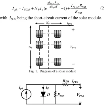
Because the output voltage of a solar cell is extremely low (about 0.5–0.7V), solar cells have to be connected in series and in parallel in practical applications first. After connection,
solar cells have to be strengthened by a supported substrate and covered by tempered glass in order to comprise the solar module (Fig. 1). After this, solar modules can be connected in series and in parallel to create a solar array according to capacity demands. At present solar modules are combined with architecture, such as walls and rooftops, in order to achieve the broadest development.
Each solar cell can be represented as a structure consisting of a photocurrent source, diode and resistors. Therefore, the equivalent circuit of a solar module [5], [6] can be shown in Fig. 2.
According to the equivalent circuit shown in Fig. 2, the relationship between output voltage and output current of the solar module is as follows [5], [6]:
PM SM PVB kT PVB
nN R I V q o P ph
PVB R
R I e V
I N I
I S
SM PVB
PVB − − +
−
=
+
) 1 (
) (
(1) with
IPVB: output current of the solar module (A).
VPVB: output voltage of the solar module (V).
Iph: current source of the solar module by solar irradiance (A).
Io: reverse saturation current of a diode (A).
NP: parallel connection number of the solar module.
NS: series connection number of the solar module.
n: ideality factor of the diode (n = 1~2).
q: electric charge of an electron (1.6×10⁻¹⁹C).
k: Boltzmann's constant (1.38×10⁻²³J/oK).
T: absolute temperature of the solar cell (oK).
RSM and RPM are the internal series resistance and parallel resistance, respectively, of the solar module. Since the value of RSM is usually small and the value of RPM is usually very large, RSM and RPM are negligible under ideal conditions. In order to make the simulation results more realistic in this paper, RSM and RPM are considered to be included in an equivalent circuit. The equation of the photocurrent source can be expressed as
PM SM kT SCM
nN R qI o P SCM
ph R
R e I
I N I
I S
SM SCM
+
− +
= ( 1) (2)
with ISCM being the short-circuit current of the solar module.
Fig. 1. Diagram of a solar module
Fig. 2. The equivalent circuit of a solar module
Since the open-circuit voltage and short-circuit current of the solar module are dependent on the variation of solar irradiance and temperature, the equation of open-circuit voltage and short-circuit current of the solar module can be derived from the following expressions:
) 1000 ( C ref
SCM ISCB T T
S
I = +α − (3) )
( C ref
OCB
OCM V T T
V = +β − (4) with
ISCB: short-circuit current of the solar module under the conditions of reference temperature and 1000W/m2. VOCM: open-circuit voltage of the solar module.
VOCB: open-circuit voltage of the solar module under the conditions of reference temperature and 1000W/m2. S: solar irradiance (W/m2).
Tref: reference temperature of the solar module (25oC).
TC: temperature of the solar module.
α: temperature coefficient of the short-circuit current for the solar module (mA/ oC).
β: temperature coefficient of the open-circuit current for the solar module (V/ oC).
The output power of the solar module can be expressed as follows:
PM SM PVB PVB kT PVB
nN R I V q o PVB P ph PVB PVB PVB
PVB R
R I V e V
I V N I V I V
P S
SM PVB
PVB ( )
) 1 (
)
( − − +
−
=
=
+
(5) In the following section, Matlab/Simulink is used to set up the solar module model as well as to simulate the I-V curve and output power of the solar module according to the equations derived above. The test solar module used in this paper is HIP-200NHE1 HIT (Heterojunction with Intrinsic Thin Layer), manufactured by SANYO Electric Company.
The electrical parameters of the test solar module were measured by SANYO Electric Company under the reference conditions (AM1.5, irradiance of 1000W/m2 and temperature of 25oC) as shown in TABLE I.
Fig. 3 shows the comparisons of I-V curves for simulation results and original field test data of the test solar module under fixed temperature of 25oC and the variation of solar irradiances. Fig. 4 shows the comparisons of I-V curves for simulation results and original field test data of the test solar module under fixed irradiance of 1000W/m2 and a variety of temperatures. According to Fig. 3 and Fig. 4, the simulated I- V curves of the proposed solar module model in this paper match very closely the measured I-V curves of SANYO’s field test data under different irradiance and temperature conditions. The proposed solar module is, therefore, validated to be accurate and practicable.
TABLEI
ELECTRICAL PARAMETERS OF THE SANYOSOLAR MODULE
Parameter Value
Maximum power (Pmax) 200 (W)
Max. power voltage (Vmp) 40.0 (V) Max. power current (Imp) 5.00 (A) Open-circuit voltage (VOC) 49.6 (V)
Short-circuit current (ISC) 5.50 (A) Temperature coefficient of ISC 1.65 (mA/oC)
Temperature coefficient of VOC -0.129 (V/oC)
Fig. 3 Comparisons of the I-V curves of the test solar module under fixed temperature and different irradiance conditions
Fig. 4. Comparisons of the I-V curves of the test solar module under fixed irradiance and different temperature conditions
III. MODELING OF ADC-DCBUCK-BOOST CONVERTER Generally speaking, the output voltage of a typical photovoltaic system is usually less than that of its load.
Therefore, a DC-DC boost converter is used as the maximum power point tracker in most photovoltaic systems. In order to extend the applicability of the photovoltaic simulation system proposed in this paper, a DC-DC buck-boost converter is used as the maximum power point tracker in the photovoltaic system model.
A DC-DC buck-boost converter is a switched-mode converter that periodically cycles the operation of an electrical switch on and off. The output voltage of this converter can be greater or less than the input voltage of the converter. A DC- DC buck-boost converter with a maximum power point tracking algorithm can adjust the output voltage of the solar module in order to operate on maximum power point in the photovoltaic system.
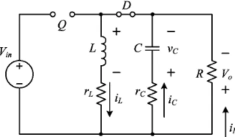
The circuit diagram of the DC-DC buck-boost converter is shown in Fig. 5 [7], [8]. The rL and rC shown in Fig. 5 represent the parasitic resistors of inductor L and capacitor C respectively. The DC-DC buck-boost converter used in this paper is operated in continuous current mode (CCM), and the parasitic components are also included in the converter model to conform realistic circuit operation.
The power switch Q is an electronic switch, usually a field effect transistor (MOSFET) or, at higher power levels, an insulated gate bipolar transistor (IGBT). This switch is able to switch on and off at high speed, with low resistance when on and very high resistance when off. The power switch operation can be divided into two states:
A. The power switch Q is turned on
When the power switch Q is turned on, the diode is cutoff due to reverse-biased voltage. The equivalent circuit of the converter is shown in Fig. 6.
The state-space equation of DC-DC buck-boost converter can be derived in the following section. According to Kirchhoff’s voltage law, the voltage across the inductor L can be expressed as
L L in
L V i r
v = − (6) Since
dt Ldi
vL = L , (2) can be modified to
( in L L)
L V i r
L dt
di = 1 −
(7) According to Kirchhoff’s current law, the current of the capacitor C can be expressed as
C R C
C R r
i v
i =− =− + (8) Equation (8) can be modified to
C C C
r R
v C dt dv
− +
= 1
(9) The output voltage of the converter can be expressed as
C C
o v
r R V R
= + (10) B. The power switch is turned off
When the power switch Q is turned off, the diode is conducted due to forward-biased voltage. The equivalent circuit of the converter is shown in Fig. 7. According to Kirchhoff’s current law, the current of the inductor L can be expressed as
Fig. 5. The circuit of the DC-DC buck-boost converter
Fig. 6. The equivalent circuit of the DC-DC buck-boost converter when the power switch is closed
Fig. 7. The equivalent circuit of the DC-DC buck-boost converter when the power switch is opened
R dt r Cdv v dt Cdv i i
i C
C C R C
C L
+ +
= +
= (11)
Equation (11) can be modified to
⎟⎟⎠
⎜⎜ ⎞
⎝
⎛
− +
= + C
C L
C
C v
r i R r R
R C dt
dv 1 1 (12)
According to Kirchhoff’s voltage law, the loop of the inductor L and capacitor C can be expressed as
=0 + +
+ L C CC
L
L v i r
dt Ldi r
i (13)
Equation (13) can be rearranged to
⎟⎟⎠
⎜⎜ ⎞
⎝
⎛
+ + +
+
− +
= C
C L C
C L C L
L v
r R i R r R
Rr r r Rr L dt
di 1 (14)
The output voltage of the converter can be expressed as
C C C L
o C v
r R i R r R V Rr
+ +
= + (15) By adding switching control parameter u and rearranging (7), (9), (12) and (14), the derivative of iL and vC can be expressed as
( )( L L C)
C
C Ri Ri u v
r R C dt
dv − −
= 1+
(16)
]}
) (
1 [ 1{
u Rv Rv i Rr r r Rr u i r Rr u R L V dt di
C C L C L C L L C C
L i − + + − +
+ +
= (17)
When the DC-DC buck-boost converter operates in steady-state, the net change of the inductor current over one period should be zero; that is,
( ) ( )ΔiL on+ ΔiL off =0 (18)
(1 ) 0
)
(− − =
+ L
T D V L
DT
Vin o
(19) The output voltage of the converter can be derived from (19) and is expressed as
in
o V
D V D
= −
1 (20) with
T t t t
D t on
off on
on =
= + ; 10< D< ; D is the duty ratio.
The Vin and Vo in (20) indicate magnitude of input and output voltage, respectively, of the converter. According to
Figs. 5 to 7, the output voltage Vo has opposite polarity from the input voltage Vin. Output voltage magnitude of the buck- boost converter could be greater or less than the source voltage, depending on the duty ratio of the switch. If D > 0.5, Vo is greater than Vin. If D < 0.5, Vo is less than Vin.
The operation of the DC-DC buck-boost converter used in this paper is in CCM, the minimum inductance and capacitance designed to generate continuous current can be expressed as [8]
( )
f R L D
2
1 2
min = − (21)
) /
min (
o o V V Rf C D
= Δ (22) with
o o
V
ΔV : output voltage ripple
In order to verify the correctness of the DC-DC buck-boost converter model proposed in this paper, a test case is performed in the following section. The input voltage of the test case is 40V, and the output voltages are set to be 60V and 20V respectively. The load resistance, switching frequency and output voltage ripple are set to be 50Ω, 25Hz and 1%
respectively. The minimum value of inductance and capacitance of the converter can be calculated by (21) and (22).
The appropriate parameters chosen for the DC-DC buck- boost converter in the test case are listed in TABLE II. The converter simulation results for voltage step-up and voltage step-down are shown in Fig. 8. According to Fig. 8, it can be observed that the buck-boost converter can transform the source voltage to 60V (voltage step-up) and 20V (voltage step-down) successfully. The correctness of the DC-DC buck- boost converter model is therefore validated.
IV.THE ALGORITHM OF MAXIMUM POWER POINT TRACKING
The method used in this paper to implement maximum power point tracking function is the perturbation and observation method [3], [9], [10], which is the most popular method. The advantages of the perturbation and observation method include simple structure, less measured parameters and no need of measurement in advance.
By continuously perturbing the output power of the solar module, the perturbation and observation method could find the location of maximum power point and send a control signal to the DC-DC buck-boost converter through a PWM controller to modulate the operating point of the solar modules.
The basic algorithm of the perturbation and observation method is to periodically vary the duty ratio in order to adjust the voltage across the solar module, and hence the module current and power.
TABLEII
PARAMETRES OF THE DC-DCBUCK-BOOST CONVERTER
Parameter Value Input voltage (Vin) 40.0 (V) Load resistance (R) 50 (Ω)
Inductance (L) 0.16 (mH)
Capacitance (C) 48 (μF)
Switching frequency (f) 25 (kHz)
Fig. 8. Output voltage of the DC-DC buck-boost converter
The magnitudes of output voltage and power before and after the variation of duty ratio are observed and compared in order to determine that the duty ratio should be increased or decreased for the following perturbation. By using the procedures of perturbation, observation and comparison again and again, the output power of the solar modules can then reach its maximum working point gradually. The flow chart of the perturbation and observation method is shown in Fig. 9.
V. SIMULATION OF THE PHOTOVOLTAIC SYSTEMS
In order to verify the effect of the MPPT for the photovoltaic simulation system, some test cases are implemented under different irradiance, temperature and load conditions to observe whether the output power (load power) of the photovoltaic simulation system can reach the maximum power of the solar modules or not. The solar module used in the following test cases is the same as that used in Chapter II.
The schematic diagram of the photovoltaic simulation system is shown in Fig. 10.
Fig. 9. Flow chart of the perturbation and observation method
Fig. 10. The schematic diagram of the photovoltaic simulation system
A. Voltage step-up cases
1) Irradiance: 1000W/m2; temperature: 25oC; load: 10Ω
Fig. 11. The comparison of output power for the photovoltaic system with and without MPPT.
2) Irradiance: 700W/m2; temperature: 28oC; load: 15Ω
Fig. 12. The comparison of output power for the photovoltaic system with and without MPPT.
B. Voltage step-down cases
1) Irradiance: 800W/m2; temperature: 23oC; load: 5Ω
Fig. 13. The comparison of output power for the photovoltaic system with and without MPPT.
2) Irradiance: 300W/m2; temperature: 20oC; load: 20Ω
Fig. 14. The comparison of output power for the photovoltaic system with and without MPPT.
According to the comparisons of the simulation results shown in Figs. 11 to 14, the photovoltaic system with MPPT function can supply more power to resistive load than the system without MPPT function. By comparing the output power diagram and P-V diagram in each test case, it can be observed that the photovoltaic simulation system could successfully track the maximum power under different weather conditions. The applicability and correctness of the photovoltaic simulation system are validated. Since the parasitic resistors of the inductor and capacitor are included in the DC-DC buck-boost converter model, the output power tracked by the MPPT in each of the simulation diagrams is less than the ideal maximum power. Therefore, the simulation
results of the photovoltaic simulation system established in this paper are more consistent with the actual situation of the photovoltaic system.
VI. CONCLUSION
The main purpose of this paper is to establish a model for a photovoltaic system with maximum power point tracking function completely through the use of software techniques. A model of a solar module was first established and then combined with an MPPT algorithm, as well as models of a PWM controller and a DC-DC converter, in order to set up a complete photovoltaic simulation system. In order to extend the operation range of the photovoltaic simulation system, a DC-DC buck-boost converter with perturbation and observation capabilities is used in this paper to implement the MPPT task.
The simulation result diagrams shown in the paper not only verify the accuracy of the characteristics for the established solar module model, but also prove that the photovoltaic simulation system can approximately track the maximum power point rapidly and successfully under different test conditions. The correctness and practicability of the photovoltaic simulation system established in this paper are then validated. According to Figs. 11 to 14, it can be observed that the tracked power is less than the ideal maximum power in each test case. The power losses are due to the parasitic resistance effect of the inductor and capacitor shown in the DC-DC buck-boost converter circuit. Therefore, the simulation results of the photovoltaic system with MPPT
function established in this paper show agreement with the real power generation situations.
REFERENCES
[1] Y. Yusof, S. Sayuti, M. Latif, and M. Wanik, “Modeling and simulation of maximum power point tracker for photovoltaic system,”
in Proceedings of Power and Energy Conference, Nov. 2004, pp. 88–
93.
[2] H.-L. Tsai, C.-S. Tu, and Y.-J. Su, "Development of Generalized Photovoltaic Model Using MATLAB/SIMULINK," in Proceedings of the World Congress on Engineering and Computer Science, Oct. 2008, pp. 846–854.
[3] C. Hua, J. Lin, and C. Shen, "Implementation of a DSP-controlled photovoltaic system with peakpower tracking," IEEE Transactions on Industrial Electronics, Vol. 45, no. 1, pp. 99–107, Feb. 1998.
[4] K.H. Hussein, I. Muta, T. Hoshino, and M. Osakada, "Maximum photovoltaic power tracking: an algorithm for rapidlychanging atmospheric conditions," IEE Proceedings-Generation, Transmission and Distribution, Vol. 142, no. 1, pp. 59–64, Jan. 1995.
[5] F. Lasnier, T. G. Ang, Photovoltaic Engineering Handbook, New York:
IOP Publishing Ltd, 1990.
[6] L. Castaner and S. Silvestre, Modelling Photovoltaic Systems Using PSpice, West Sussex, England: John Wiley & Sons Ltd, 2002.
[7] M.H. Rashid, Power Electronics Circuits: Devices and Applications, 3rd edition, Upper Saddle River, NJ: Prentice-Hall, 2004.
[8] D.W. Hart, Introduction to Power Electronics, Upper Saddle River, NJ:
Prentice-Hall, 1997.
[9] Y.-T. Hsiao and C.-H. Chen, “Maximum Power Tracking for Photovoltaic Power Systems,” in Proceedings of the IEEE 37th IAS Annual Meeting, vol. 2, Oct. 2002, pp. 1035–1040.
[10] M. El-Shibini and H. Rakha, "Maximum Power Point Tracking Technique,” in Proceedings of Electrotechnical Conference, Apr. 1989, pp. 21–24.