Volume19, No1, November 2014, pp. 49-62
1 Ph.D., Department of Geomatics, National Cheng Kung University Received Date: Apr. 08, 2013
2 Professor, Department of Geomatics, National Cheng Kung University Revised Date: Feb. 10, 2014
2 Professor, School of Civil Engineering and Geosciences, Newcastle University, Accepted Date: Oct. 21, 2014
*.Corresponding Author, Phone: 886-6-2373876 ext. 852, E-mail: miaowang@geomatics.ncku.edu.tw
Extraction of Surface Features from LiDAR Point Clouds Using Incremental Segmentation Strategy
Miao Wang 1* Yi-Hsing Tseng 2
ABSTRACT
LiDAR (Light Detection and Ranging) point clouds are measurements of irregularly distributed points on scanned object surfaces acquired with airborne or terrestrial LiDAR systems. Feature extraction is the key to transform LiDAR data into spatial information. Surface features are dominant in most LiDAR data corresponding to scanned object surfaces. This paper proposes a general method to segment co-surface points. An incremental segmentation strategy is developed for the implementation, which comprises several algorithms and employs various criteria to gradually segment LiDAR point clouds into several levels. There are four operation steps. First, the proximity of point clouds is established as spatial indices defined in an octree-structured voxel space. Second, a connected-component labeling algorithm for voxels is applied for segmenting neighboring points.
Third, coplanar points then can be segmented with the octree-based split-and-merge algorithm as plane features. Finally, combining neighboring plane features forms surface features. With respect to each step, processed LiDAR point clouds are segmented into organized points, neighboring point groups, coplanar point groups, and co-surface point groups. The proposed method enables an incremental retrieval and analysis of a large LiDAR dataset. Experiment results demonstrate the effectiveness of the segmentation algorithm in handling both airborne and terrestrial LiDAR data. The end results as well as the intermediate results of the segmentation may be useful for object modeling of different purposes using LiDAR data.
Keywords: LiDAR Point Cloud, Segmentation, Octree, Voxel Space, Spatial Feature, Incremental
1. Introduction
Light detection and ranging (LiDAR) is an advanced and efficient technology for the acquisition of three-dimensional (3D) spatial data by airborne or terrestrial LiDAR systems since the late twentieth century (Ackermann, 1999). The point measurements acquired are also known as point clouds. A typical LiDAR point records both the geometric and radiometric properties of the scanned object. The 3D coordinates of LiDAR points implicitly describe the geometric properties of objects, and the intensity data of a reflected laser pulse present the radiometric properties of objects. The 3D coordinates of each point contain certain random error that results from laser ranging and scanning error and may also contain systematic errors from imperfect system installation or calibration.
As collections of surface point
measurements of scanned objects distributed in 3D space, LiDAR data are the digital surface models of the scanned targets. A common LiDAR point cloud may contain the points of natural objects, such as the terrain and trees, and man-made objects, such as buildings, roads, bridges, and pipelines. LiDAR point clouds implicitly contain abundant spatial information about the scanned targets that can be exploited through various data processing methods for applications such as digital elevation model (DEM) generation (Sithole and Vosselman, 2004), 3D building modeling (Chio, 2008), forestry management (Maas et al., 2008), transportation network design (Oude Elberink and Vosselman, 2009), power line extraction (McLaughlin, 2006), and reconstruction of industrial installations (Rabbani, 2006). For every LiDAR data application, the ultimate objectives are the identification and recognition of the contents in the data (Vosselman et al.,
2004). The process can be regarded as the interpretation of LiDAR data.
For 3D city modeling, terrain and buildings are the objects of most interest. The extraction of spatial features is often the first task in the reconstruction of 3D object models using LiDAR data. A visual inspection of LiDAR data easily reveals the shapes and appearances of the scanned targets. From the geometric point of view, although the shapes of the terrain and buildings vary and are sometimes very complex, they are composed of basic geometric primitives, namely surfaces, lines, and points. Therefore, it is often preferable to model objects using compact models, such as a boundary representation (B-rep), to simplify the models and reduce the required storage space (Rottensteiner and Clode, 2008). 3D object models can then be reconstructed based on these spatial features.
Because the points are mainly distributed on the surfaces of scanned objects and are difficult to locate on the edges or vertices of objects accurately due to the inherent properties of laser scanning mechanism, surfaces features are the dominant spatial features that can be extracted from LiDAR data. Segmentation is the most commonly used method for extracting surface features from LiDAR point clouds. The point distribution is the major attribute used for segmenting LiDAR data. Segmentation algorithms segment point clouds into point groups based on the proximity and coherence of points; i.e., the points in a group are neighboring points with similar properties (Melzer, 2007).
Each segmented point group represents a spatial feature of the point distribution that is composed of coherent points. For the extraction of surface features, points distributed on a common surface are defined as being coherent. The segmentation results are groups of co-surface points related to surface features; the surface features are thus extracted. Similarly, segmentation that defines coplanar points as being coherent is used to extract planar features. The proximity of points is also known as the neighborhood of points. In a point cloud, two points are regarded as neighbors if the distance between them is shorter than a distance threshold. The distance threshold is usually related to the point spacing of the point cloud.
During a segmentation procedure, points must be retrieved from point cloud in 3D space to determine the neighboring points of each
point. Because a common LiDAR point cloud often has a very large number of points and the distribution of points is not uniform, searching for points is not an easy task. An additional data structure is thus required for handling points.
Many data structures have been used for the segmentation of point clouds. The design of data structures is strongly related to the design of segmentation algorithms. Earlier studies for segmentation of point clouds are performed on range images obtained from range cameras (Hoover et al., 1996). The inherent 2D data structure of the range image provides a regular spatial index for segmentation algorithms.
Segmentation concepts and algorithms designed for 2D images, such as clustering, region growing, and split-and-merge, have been modified and implemented for range images.
Segmentation algorithms for LiDAR point clouds are mainly adapted from those for range images. However, because most LiDAR point clouds are not stored in 2D arrays, the algorithms must be modified to employ data structures suitable for handling the neighborhood of the points. The triangulated irregular network (TIN) (Pu and Vosselman, 2006) or interpolated grid data structure (Chen, 2007) are often used for handling 2.5D airborne LiDAR point clouds. A k-d tree is often used to determine the k-nearest neighbors (k-NNs) of each point. Data structures and regular spatial indexing, such as quadtrees and octrees, are usually used to determine the fixed distance neighbors (FDNs) of points (Rabbani, 2006).
Filin and Pfeifer (2006) proposed a slope adaptive neighborhood to select appropriate neighboring points for the segmentation of airborne LiDAR point clouds. For the segmentation of points without regular order, a general 3D data structure is suitable for building neighborhoods of points (Bucksch et al., 2009).
Therefore, a 3D data structure called voxel space or 3D grid is used for organizing unordered point clouds in this study.
The strategy used to treat the proximity and coherence of points in LiDAR data segmentation is also important. Although the proximity and coherence of points are both required criteria for segmentation, they can be processed separately at different steps using different algorithms.
Therefore, the segmentation of LiDAR point clouds can be separated into several steps that employ different algorithms and the criteria of proximity and coherence to generate
Using Incremental Segmentation Strategy
segmentation results in an incremental fashion.
This study develops a general-purpose incremental segmentation scheme for segmenting co-surface points from general LiDAR data. A common LiDAR point cloud usually contains a large number of points of various spatial features which are difficult to well segment simultaneously using only one segmentation algorithm. In this study, the segmentation thus integrates several segmentation algorithms with different criteria of proximity and/or coherence step by step according to the given application. For each segmentation step, different criteria are gradually introduced to generate incremental results. The designed incremental segmentation strategy has three important properties. First, the segmentation algorithms use a common data structure so that the proximity of points can be determined on the same basis. Second, each segmentation step generates specific results with particular properties by using different combinations of proximity and/or coherence criteria for different purposes. Third, the results obtained at each step are used as the foundation data for the following step, thus incrementally generating the segmentation results. Based on these considerations, the number of segmentation steps, the type of segmentation algorithm, and the criteria used at each step depend on the purpose of segmentation.
2. Methodology
Wang and Tseng (2011) proposed a four-step incremental segmentation strategy for the segmentation of co-surface points of general surfaces. This segmentation strategy gradually produces incremental results step by step using different algorithms and criteria of coherence and proximity, allowing the results obtained in a given step to be the input data for the next step.
The details of each step are described in the follows.
2.1 First Step: Organizing a Point Cloud with Regular Grids
The distribution of LiDAR point clouds is usually anisotropic. Airborne LiDAR points are usually recorded one by one in sequence rather than in a regular gridded format. Some studies have interpolated airborne LiDAR points into regular 2D grids (Miliaresis and Kokkas, 2007).
Although data processing for gridded data can
be easily implemented using mature image processing tools, the source data are distorted due to the interpolation, which influences the quality of the processing results. Point clouds obtained from most terrestrial laser scanners are designed to be recorded with 2D-array data structures. However, the benefits of the 2D gridded data structure are lost if the point set is arbitrarily cut from the original point cloud or is a registered point cloud combined with several scans.
At this study, an octree-structured voxel (volumetric element) space is used for the organization of both airborne and terrestrial LiDAR point clouds. The purpose of organizing LiDAR point clouds using the voxel space is to reorder the sequence of points to provide an efficient spatial index for accessing points. After the organization, point searching can be accelerated through the octree structure.
To organize a point cloud using the voxel space, the 3D space occupied by the point cloud is partitioned into connected and equal-size subspaces. Each subspace is a voxel and is regarded as a container that may contain any number of points (including none). After the organization, all points are sorted in descending order according to the spatial index of their voxel. This puts the sequence of the reordered points in the Morton order. Points inside a given voxel are sorted together in the reordered point sequence. Because the points of a common point cloud are mainly distributed on the surfaces of the scanned objects, most points are located in a few voxels (i.e., most voxels are empty).
Recording the voxel space using a standard 3D array is thus inefficient. Instead, an octree structure can be used to record the constructed voxel space. Each voxel of the voxel space is recorded as a leaf node of the octree. Fig. 1 illustrates the concept of organizing a point cloud with the octree-structured voxel space. Fig.
1 (a) shows a profile of an airborne LiDAR point cloud covering buildings, trees, cars, and the terrain. Figs. 1 (b) and (c) show the corresponding octree representation of a part of the voxel space and the Morton order of voxels containing the points, respectively.
Determining point neighborhoods is one of the major tasks in the segmentation of LiDAR point clouds. If the distance between two points is smaller than a defined threshold, the points are considered neighboring points; otherwise, they are non-neighboring points. The distribution of
LiDAR points is usually uneven so that the distances between pairs of points vary.
Practically, it is infeasible to calculate the distance between each pair of points for a large point cloud. An appropriate threshold for determining point neighborhoods is thus required. The threshold is usually defined according to the average point spacing of the original dataset. Points of airborne LiDAR point clouds are mainly distributed on the surfaces of the terrain and objects. The average point density of the point cloud, i.e., the number of points per square meter of the horizontal plane, is usually used as the quality measure of the distribution of a point cloud. The average point spacing can be determined from the average point density. Because the distribution of points is not even, the derived average point spacing may not represent the actual point spacing. In real cases, the determination of the average point density for point clouds that contain empty areas,
such as water, is not very precise. The scanning pattern and the distributions of point clouds varies with the terrestrial LiDAR system. The point density and the point spacing are difficult to determine for terrestrial LiDAR point clouds because there is no reference plane for determining the average point density.
In a 2D image, the adjacency of pixels is defined by 4- or 8-connectivity. Similarly, the adjacency of voxels is defined by 6-, 18- or 26-connectivity (Fig. 2). Because the voxel space is recorded using an octree structure, the adjacency of voxels can also be represented using the adjacency of nodes. Retrieving the adjacent voxels of a voxel in an octree-structured voxel space can be achieved using two methods, one which uses the spatial index of the voxels and one which uses the node relationship of the octree (Samet, 1990).
Figure 1. (a) Constructing a voxel space for a point cloud (side view); (b) octree presentation of a part of the voxel space (to simplify the drawing, a quadtree is drawn instead of an octree); (c) the corresponding Morton order of some voxels. (adapted from Wang and Tseng (2011))
Figure 2. Neighborhoods of a voxel: (a) 6-neighborhood; (b) 18-neighborhood; (c) 26-neighborhood (adapted from Lohmann (1998)).
2.2 Second Step: Segmentation of a Point Cloud Based on Proximity of Points
1 1 1 4, 0
4, 1 5, 0
I,K Layer 0 Layer 1 Layer 3
Layer 2
Index of node (voxel)
1 Leaf node and number of contained points
Branch node containing no point Branch node containing point(s) I(X)
K(Z)
(a)
(b) 1
0 2 3 4 5 6 7 0
1 5
2 3 4 6 7
9
8 10 11 1213 14 1516171819
1 1 0 0 0 0 0 0 0 1 0 0 0 0 0 0 0,
0
3, 3 2, 3 3, 2 2, 2 1, 3 0, 3 3, 1 2, 1 3, 0
1, 2 2,
0
0, 2 1,
1, 1 0
0 5, 1
4, 0
4, 1 5,
0 0,
0 1, 2 1, 0
7, 2
1, 4 0, 4 6,
0 6, 2 4, 2
4, 4
4, 5 5,
4 2,
5 3, 6 2, 6
9, 2 6, 6
8, 2
11,0
(c) 0,
1
(a) (b) (c)
Using Incremental Segmentation Strategy
A visual inspection of a common LiDAR point reveals that the distribution of points is not uniform and that the points can be separated into several groups of neighboring points. The scanning manner of LiDAR systems is mostly responsible for the uneven point distribution pattern. Point clouds obtained from airborne LiDAR systems may contain building shadows due to the occlusion of the laser beams (Shih and Huang, 2009). The point spacing of vertical surfaces is rather large because these surfaces are nearly parallel to the direction of the laser beam. Terrestrial laser scanning has issues of point undersampling and varying point density (Bucksch et al., 2009).
Closely distributed points often tend to belong to the same surface. In some cases, the points of a surface may be distributed far apart due to some scanning occlusions. Because proximity of points is a necessity for the segmentation, there is no need to process non-neighboring points simultaneously. For datasets with a large number of points, it is helpful to separate non-neighboring points and to group neighboring points before the segmentation. The grouping of neighboring points can be regarded as segmentation based on proximity. This segmentation allows point clouds of a large number of points to be processed and undesired segmentation results caused by inappropriate point neighborhoods to be eliminated.
Once a point cloud is organized using the octree-structured voxel space, the point neighborhood of the point cloud can be substituted using the adjacency of voxels.
Therefore, the grouping for neighboring points may be achieved by grouping adjacent voxels using the connected-component labeling (CCL) algorithm (Lohmann, 1998). Fig. 3 shows the results of CCL of the example data shown in Fig.
1. The example data are separated into several
groups of neighboring points that belong to different surfaces, such as a gable roof, curved roof, tree crown, and the terrain. Notice that points of the terrain are separated from non-terrain points because there is an insufficient number of dense vertical points for airborne LiDAR point clouds. Therefore, the voxels of terrain points and non-terrain points are not connected.
The voxel size is critical to the results of CCL. A voxel size that is either too large or too small may lead to undesired results, as shown in Fig. 3 (b) and Fig. 3 (c), respectively. The larger voxel size groups more points to a group and generates fewer point groups. Some points belonging to different surfaces or objects are grouped into the same group. For example, in Fig. 3 (b), the points of the curved roof are grouped with the terrain point groups. If the voxel size is smaller than the point spacing, CCL obtains over-segmented results of piecewise groups of points. In Fig. 3 (c), the points of the gable roof, curved roof, and the terrain are all separated into an excessive number of point groups after CCL. An appropriate voxel size for CCL should be set according to the point spacing of the point cloud. The voxel size must be a little larger than the average point spacing derived from the average point density for airborne LiDAR point clouds. However, there is no rule for automatically determining the appropriate voxel size for terrestrial point clouds.
When an appropriate voxel size is set, CCL for voxels can be used for the neighboring test of points to determine whether the points of a dataset are all neighboring points. If the voxels containing these points are all connected, i.e., only one connected voxel group is obtained using the CCL algorithm, these points are neighboring points and pass the neighboring test.
(a) (b) (c)
Figure 3. Voxel and point group results of CCL for an (a) suitable and excessively (b) large and (c) small voxel size. (adapted from Wang and Tseng (2011))
2.3 Third Step: Segmentation of Coplanar Points
Previous studies on the segmentation of LiDAR point clouds have mostly focused on the segmentation of coplanar points. Wang and Tseng (2010) proposed a segmentation method called the octree-based split-and-merge algorithm for the automatic extraction of plane features from unstructured LiDAR point clouds.
At this study, the algorithm is extended to the octree-structured voxel space.
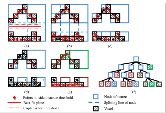
The algorithm includes two major recursive processes: split and merge. The split process explores coplanar point patches from the point cloud by recursively examining the coplanar properties of point distribution and splitting the point set. Then, in the merge process, neighboring coplanar point patches are merged to form coplanar point groups to complete the segmentation. At both the split and the merge processes, the criteria of coherence and proximity are used for the segmentation.
Principal component analysis (PCA) is applied to determine the best-fit plane of the points. A coplanar test is used to evaluate the quality of the fitting plane (Rabbani, 2006). Then, the connected component labeling algorithm is used to check the proximity of the voxels and points.
During the split process, the built octree-structured voxel space is used for
recording the splitting results and is the kernel structure throughout the algorithm. The spatial indices of the octree-structured voxel space provide efficient access to the points throughout the segmentation procedure. Because the proposed algorithm employs a 3D data structure, the octree structure, for organizing point clouds, it can be applied to both airborne and terrestrial LiDAR point clouds without modification. The algorithm can be performed without scan-line information.
Fig. 4 shows an example of the split-and-merge algorithm for points of a gable roof building. Fig. 4 (a) shows the space containing all points extended to a cubic space covering all the voxels. The space is recorded as the root node of the octree. A best-fit plane is determined. Since none of the points (red) contained in the root node passed the coplanar test, the space is split into 8 sub-spaces (only 4 nodes are shown). The plane fitting processes, the coplanar test, and space splitting are performed on each sub-space until points contained in all sub-spaces satisfy the stop splitting criteria (Figs. 4 (b)-(d)). The final merging result and the tree representation of the split process are shown in Figs. 4 (e) and (f), respectively.
Figure 4. Split-and-merge segmentation for the point group of a gable roof building. (a)-(d) split process; (e) results of merge process; (f) tree representation (using a quadtree for simplicity)
2.4 Fourth Step: Segmentation of Co-surface Points
Best-fit plane
Voxel
Splitting line of node Points outside distance threshold Node of octree
Coplanar test threshold
(a) (b) (c)
(e) (f)
0
1 2 11
10 9
8
6 7 4 5 2 3
1 9 10 11
12
8
3 7
1
0 2 4 5 6
(d)
Using Incremental Segmentation Strategy
The extraction of surface features from LiDAR points can be achieved by determining co-surface points from the point cloud using segmentation algorithms. In this step, the co-surface properties of points are used to gather co-surface points from the coplanar point groups obtained in the previous step. Because general surfaces have various shapes, the criteria for the co-surface property may have a variety of definitions. In this study, the criteria of the co-surface property are the included angles of the neighboring fitting planes obtained at the third step. Fig. 5 (a) shows the side view of possible results for coplanar point segmentation on the points of a curved surface. The angle
variation of two neighboring fitting planes of the coplanar point groups is the included angle of the normal vectors of the planes. An angle threshold (a) can be set to determine whether two neighboring coplanar point groups can be merged. If the angle variation is smaller than the co-surface threshold, the two point groups are merged into a co-surface point group. The value of the threshold should be determined according to the properties of the point cloud and the given application.
To summarize the four-step incremental segmentation strategy, the criteria and the input and output of the methods described above are listed in Table 1.
Table 1. Criterion and input/output data of each step
Figure 5. Criterion of co-surface points. (a) Points of a curved surface segmented into neighboring coplanar point groups; (b) included angle of normal vectors of neighboring coplanar point groups; (c) angle variation of neighboring coplanar points
3. Experiments and Discussion
An airborne LiDAR point cloud of aCoplanar test threshold Coplanar points
Direction of fitting plane
Angle variation of two fitting planes Best-fit plane
(a) 0
(b) 0
Co-surface points
(c) 0
Weight center Normal vector
Included angle of two normal vectors
Intersection line of neighboring planes
Step Criterion Input Output
1st Neighboring Unordered point cloud Organized points and octree-structured voxel space
2nd Neighboring Voxels Groups of connected voxels and corresponding neighboring points
3rd Coplanar Neighboring
Neighboring point groups
Groups of coplanar points and properties of best-fit plane: normal vector, weight center, boundary
4th Co-surface Neighboring
Normal vectors and centroids of best-fit
planes
Groups of co-surface points
campus and a terrestrial LiDAR point of a building were used to test the proposed incremental segmentation strategy.
Airborne LiDAR point cloud
This dataset is the point cloud of the Kuang Fu Campus of National Cheng Kung University;
it includes terrain, buildings and trees. The point cloud was cut from a combination of three overlapped strips. The number of points is 2,772,880 and the average density is about 10.7 pts./m2, or a point spacing of about 0.31 m. Fig.
6 (a) shows an aerial image of the test area. The red rectangle and circle in Fig. 6 (a) are a gable roof building and a curved-roof building, respectively. Figs. 6 (b) and (c) show the top view and perspective view of the point cloud, respectively.
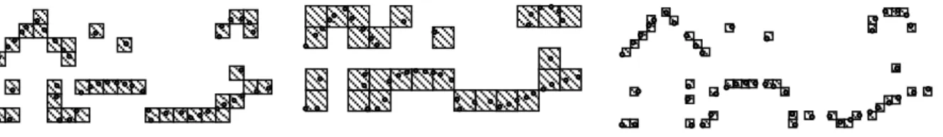
In the first step, the point cloud was organized using a voxel size of 0.5 m. The organization generated 1,484,772 voxels. In the second step, the CCL algorithm generated 35,836 neighboring point groups. Figs. 7 (a)
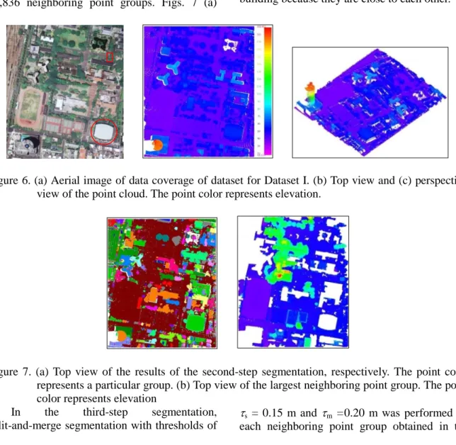
shows the top view of the results of CCL, respectively. Most points of the buildings and trees are separated from the terrain. Some points of trees are grouped with the building groups because the points are distributed close to each other. The largest and smallest point groups contain 1,599,020 and 1 points, respectively. Fig.
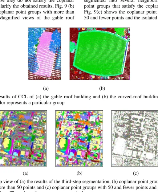
7 (b) shows the points of the largest neighboring point group. Most points in this group belong to the terrain. Some points of the buildings and trees are grouped into this group because the points of the vertical walls and trunks are dense and close to the ground that makes their voxels being connected to terrain voxels. Figs. 8 (a) and (b) show the results of CCL of the gable roof building and curved-roof building, respectively.
Points of the gable roof are grouped into the same group and separated from points of the trees and the terrain. Points of the curved-roof building are also separated from the trees and the terrain. However, some points of the trees are grouped with points of the eaves of the building because they are close to each other.
Figure 6. (a) Aerial image of data coverage of dataset for Dataset I. (b) Top view and (c) perspective view of the point cloud. The point color represents elevation.
Figure 7. (a) Top view of the results of the second-step segmentation, respectively. The point color represents a particular group. (b) Top view of the largest neighboring point group. The point color represents elevation
In the third-step segmentation, split-and-merge segmentation with thresholds of
s = 0.15 m and m =0.20 m was performed on each neighboring point group obtained in the
Using Incremental Segmentation Strategy
second step. Fig. 9 (a) shows the resulting coplanar point groups. Points of the buildings and trees are separated from the ground point group because they do not satisfy the coplanar criteria. To clarify the obtained results, Fig. 9 (b) shows the coplanar point groups with more than 50 points. Magnified views of the gable roof
building and the curved-roof building are shown in Figs. 10 (a) and (b), respectively. As described in Section 4, points of the curved surface are segmented into several neighboring coplanar point groups that satisfy the coplanar criterion.
Fig. 9(c) shows the coplanar point groups with 50 and fewer points and the isolated points.
(a) (b)
Figure 8. Results of CCL of (a) the gable roof building and (b) the curved-roof building. The point color represents a particular group
(a) (b) (c)
Figure 9. Top view of (a) the results of the third-step segmentation, (b) coplanar point groups with more than 50 points and (c) coplanar point groups with 50 and fewer points and isolated points. The point color represents a particular group
(a) (b)
Figure 10. Results of the third-step segmentation of (a) the gable roof building and (b) the curved-roof building. The point color represents a particular group
In the fourth-step segmentation, the neighboring coplanar point groups obtained in the third step are merged to form co-surface
point groups with a threshold a = 10°. Fig. 11 shows the resulting co-surface point groups. The points of the ground are merged into one group.
Magnified views of the gable roof building and the curved-roof building are shown in Figs. 12 (a) and (b), respectively. The points of the curved roof are merged into one co-surface group because the neighboring coplanar point groups satisfy the co-surface criterion. The points of the gable roof are merged into the four main coplanar point groups because the included angles of the best-fit plane of these point groups are larger than the co-surface criterion. Fig. 11 (b) shows the co-surface point groups with more than 50 points and Fig. 11 (c) show the coplanar point groups with 50 and fewer points and the isolated points. Most of the points are located in the trees and the boundaries of the building, and can thus be used for building boundary and tree crown detection.
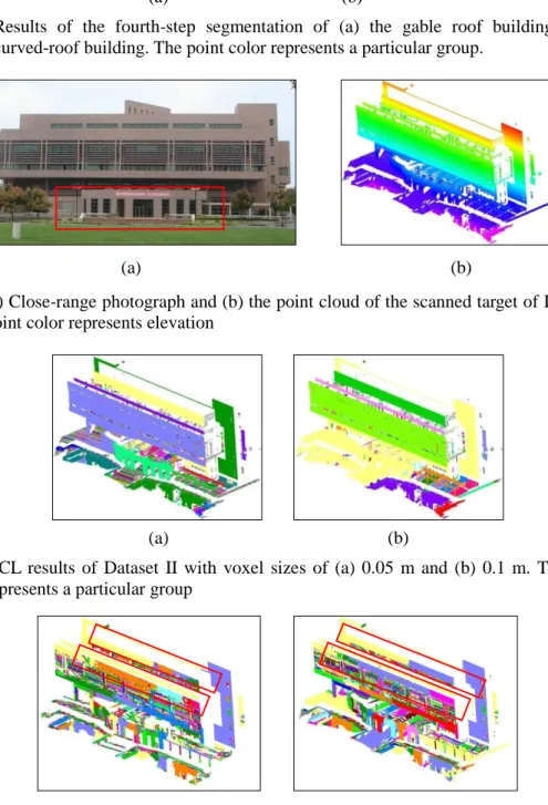
Terrestrial LiDAR point cloud
This dataset is the point cloud of the façade of the main library building of NCKU, which was cut from a scan of terrestrial LiDAR data.
Figs. 13 (a) and (b) show the close-range photograph and the point cloud of the scanned targets, respectively. The point cloud covers the façade of the building, the ground, and other objects. The façade of the building is composed of planar and curved (red rectangle in Fig. 13 (a)) surfaces. The number of points is 1,745,490. The point distribution of the walls is fairly even and dense but the point distribution of the ground is sparse. The point spacing is about 0.03m at the
wall and 0.12 at the ground along the scan direction.
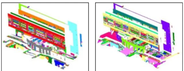
In order to determine the effect of voxel size, the point cloud was organized using voxel sizes of 0.05 m and 0.1 m, respectively. The organization generated 1,008,666 and 356,973 voxels, respectively. The CCL process generated 10,323 and 2,589 neighboring point groups for voxel sizes of 0.05 m and 0.1 m, respectively.
Figs. 14 (a) and (b) show the results of CCL for voxel sizes of 0.05 m and 0.1 m, respectively.
The points of the ground are separated into several groups when the voxel size is smaller than the point spacing (Fig. 14 (a)), and grouped together when the voxel size is larger than the point spacing (Fig. 14 (b)). In Fig. 14 (b), the points of some walls are grouped with the ground through the connection of the ground.
In the third-step segmentation, the coplanar point groups were generated using the split-and-merge segmentation algorithm with thresholds of s = 0.05 m and m =0.10 m. The split-and-merge algorithm was performed on the 343 large neighboring point groups in Fig. 15 (a) and 243 large neighboring point groups in Fig.
15 (b). The results are shown in Fig. 15. The points of the plane surfaces are segmented into large coplanar point groups. Some points of a given plane surface are not grouped into the same group because they did not pass the coplanar test or the neighboring test (red rectangles in Fig. 15). The points of curved surfaces are segmented into neighboring coplanar point groups, as expected.
(a) (b) (c)
Figure 11. Top view of (a) the results of the fourth-step segmentation, (b) co-surface point groups with more than 50 points and (c) co-surface point groups with 50 and fewer points and isolated points. The point color represents a particular group.
Using Incremental Segmentation Strategy
(a) (b)
Figure 12. Results of the fourth-step segmentation of (a) the gable roof building and (b) the curved-roof building. The point color represents a particular group.
(a) (b)
Figure 13. (a) Close-range photograph and (b) the point cloud of the scanned target of Dataset II. The point color represents elevation
(a) (b)
Figure 14. CCL results of Dataset II with voxel sizes of (a) 0.05 m and (b) 0.1 m. The point color represents a particular group
(a) (b)
Figure 15. Results of the third-step segmentation for voxel sizes of (a) 0.05 m and (b) 0.1 m. The point color represents a particular group
In the fourth step, the co-surface point groups were generated using an angle threshold
a = 10°. Fig. 16 shows the resulting co-surface point groups. Because the curvatures of the curved walls are small, the small angle threshold is sufficient to group the neighboring coplanar point groups into co-surface point groups. The separate coplanar point groups in the rectangles in Fig. 16 were merged in this step.
(a) (b)
Figure 16. Results of the fourth-step segmentation for voxel sizes of (a) 0.05 m and (b) 0.1 m. The point color represents a particular group
4. Conclusion and Future Work
Segmentation is the primary method used to extract spatial features from LiDAR data to interpret data content implied in point clouds.
Proximity and coherence of point distribution are two major criteria involved in segmentation algorithms. The data structures used to organize points for handling point neighborhood and processing strategy of algorithms are also important properties for LiDAR point cloud segmentation. At this study, a 3D data structure, octree-structured voxel space, is employed to organize LiDAR point clouds to establish neighborhoods for points. The organization is also a segmentation of points based on the proximity of point distribution. The 3D data structure can apply to both airborne and terrestrial LiDAR point clouds without modification. The octree-structured voxel space is the kernel for handling points through this study.
A four-step incremental segmentation strategy is proposed for segmentation of co-surface points. The major idea of the method is that segmentation of LiDAR point clouds can be achieved step by step using several segmentation algorithms that gradually using different proximity and/or coherence criteria of point distribution according to applications. At
this study, the segmentation integrates four segmentation methods, namely octree-structured voxel space organization, connected component labeling, octree-based split-and-merge, and a simple region growing. The four-step segmentation strategy generates incremental results, including the organized points, neighboring point groups, coplanar point groups, and co-surface point groups. The octree-structured voxel space is used for managing the proximity of points throughout the whole process. The method is implemented and tested with airborne and terrestrial LiDAR data.
The experiments demonstrate that segmentation of LiDAR point clouds can be achieved through several separated procedures with different criteria of proximity and coherence.
The current version of the incremental segmentation strategy stops at the segmentation of co-surface points. Based on the present results, some studies like detecting and grouping non-neighboring co-surface points, modeling co-surface points using a general geometric model, and detecting and modeling points of trees can be developed to further extend the research. Once the segmentation is completed segmentation-based classification is possible based on the inherent or derived features of the segmentation results. The classification can be simple (terrain or non-terrain points) or complex (recognition of scanned objects).
References
Ackermann, F., 1999. Airborne Laser Scanning - Present Status and Future Expectations.
ISPRS Journal of Photogrammetry and Remote Sensing, 54(2-3): 64-67.
Bucksch, A., Lindenbergh, R. and Menenti, M., 2009. SkelTre-Fast Skeletonisation for Imperfect Point Cloud Data of Botanic Trees, Eurographics Workshop on 3D Object Retrieval. Eurographics, München, Germany, pp. 8.
Chen, Q., 2007. Airborne Lidar Data Processing and Information Extraction.
Photogrammetric Engineering and Remote Sensing, 73(2): 109-112.
Chio, S.-H., 2008. A Study on Roof Point Extraction Based on Robust Estimation from Airborne LiDAR Data. Journal of the Chinese Institute of Engineers, 31(4):
537-550.
Using Incremental Segmentation Strategy
Filin, S. and Pfeifer, N., 2006. Segmentation of Airborne Laser Scanning Data Using a Slope Adaptive Neighborhood. ISPRS Journal of Photogrammetry and Remote Sensing, 60(2): 71-80.
Hoover, A. et al., 1996. An Experimental Comparison of Range Image Segmentation Algorithms. IEEE Transactions on Pattern Analysis and Machine Intelligence, 18(7):
673-689.
Lohmann, G., 1998. Volumetric Image Analysis, John Wiley & Sons Ltd, West Sussex, England, 243 p.
Maas, H., Bienert, A., Scheller, S. and Keane, E., 2008. Automatic forest inventory parameter determination from terrestrial laser scanner data. International Journal of Remote Sensing, 29(5): 1579-1593.
McLaughlin, R.A., 2006. Extracting Transmission Lines from Airborne LIDAR Data. IEEE Geoscience and Remote Sensing Letters, 3(2): 222-226.
Melzer, T., 2007. Non-parametric Segmentation of ALS Point Clouds Using Mean Shift.
Journal of Applied Geodesy, 1(3): 159-170.
Miliaresis, G. and Kokkas, N., 2007.
Segmentation and Object-based Classification for the Extraction of the Building Class from LIDAR DEMs.
Computers & Geosciences, 33(8):
1076-1087.
Oude Elberink, S.J. and Vosselman, G., 2009.
3D Information Extraction from Laser Point Clouds Covering Complex Road Junctions. The Photogrammetric Record, 24(125): 23-36.
Pu, S. and Vosselman, G., 2006. Automatic Extraction of Building Features from Terrestrial Laser Scanning. International Archives of Photogrammetry, Remote Sensing and Spatial Information Sciences, 36(Part 5): 5 pages (on CD-ROM).
Rabbani, T., 2006. Automatic Reconstruction of Industrial Installations Using Point Clouds and Images. Ph.D. Thesis, Delft University of Technology, 175 p.
Rottensteiner, F. and Clode, S., 2008. Building and Road Extraction by LiDAR and Image.
In: J. Shan and C.K. Toth (Editors), TOPOGRAPHIC LASER RANGING AND SCANNING Principles and Processing,
CRC Press, Boca Raton, FL, pp. 445-478.
Samet, H., 1990. Applications of Spatial Data Structures: Computer Graphics, Image Processing, and GIS, Addison-Wesley, Reading, Massachusetts, 507 p.
Shih, P. and Huang, C., 2009. The building shadow problem of airborne lidar. The Photogrammetric Record, 24(128):
372-385.
Sithole, G. and Vosselman, G., 2004.
Experimental Comparison of Filter Algorithms for Bare-Earth Extraction From Airborne Laser Scanning Point Clouds.
ISPRS Journal of Photogrammetry and Remote Sensing, 59(1/2): 85-101.
Vosselman, G., Gorte, B.G.H., Sithole, G. and Rabbani, T., 2004. Recognising Structure in Laser Scanner Point Clouds. International Archives of Photogrammetry and Remote Sensing, 36(part 8/W2): 33-38.
Wang, M. and Tseng, Y.-H., 2010. Automatic Segmentation of LiDAR Data into Coplanar Point Clusters Using an Octree-Based Split-and-Merge Algorithm.
Photogrammetric Engineering and Remote Sensing, 76(4): 407-420.
Wang, M. and Tseng, Y.-H., 2011. Incremental Segmentation of LiDAR Point Clouds with an Octree-Structured Voxel Space. The Photogrammetric Record, 26(133): 32-57.
1國立成功大學測量及空間資訊學系 博士 收到日期:民國 102 年 04 月 08 日
2國立成功大學測量及空間資訊學系 教授 修改日期:民國 103 年 02 月 10 日
3中山科學研究院資訊通信研究所 助理研究員 接受日期:民國 103 年 10 月 21 日
*通訊作者, 電話: 06-2373876 ext. 852, E-mail: miaowang@geomatics.ncku.edu.tw
使用漸增式區塊化策略從光達點雲萃取面特徵
王淼
1*曾義星
2摘 要
以空載或地面光達(Light Detection and Ranging, LiDAR)掃瞄得到的資料是不規則分佈於被 掃瞄物體表面的點觀測量,特徵萃取是將光達資料轉換為空間資訊的關鍵程序,其中面特徵是 光達資料中最主要的空間特徵。本文提出一個通用性的方法-漸增式區塊化策略-進行共面點 雲區塊化,漸增式區塊化策略可依應用需求分為數個步驟,在每個步驟採用適當的演算法和運 算條件。本研究提出的方法將面特徵萃取分為四個步驟:第一、使用八分樹結構化體元空間建 立點雲間的相鄰關係;第二、使用相連成份標記(Connected Component Labeling)演算法將點雲區 分為數個相鄰點群;第三、使用基於八分樹之分割-合併演算法從每個點群中萃取出平面特徵;
最後,使用區域成長法將相鄰的平面特徵合併為曲面特徵。實際上,四個步驟分別將光達點雲 區分為組織化的點群、相鄰點群、共平面點群及共曲面點群。利用本研究提出的方法可採漸增 方式進行大量點雲資料集之擷取及分析,實驗證明此方法可有效率地處理空載和地面光達點雲 資料,而且,本方法的最終以及中間成果均可分別應用於不同目的的物體模塑。
關鍵詞:光達點雲、區塊化、八分樹、體元空間、空間特徵、漸增式