Chapter 4 Experimental Method and Results
4.1 Equipment
In this thesis, general commercial digital camera such as Casio Z4, or special
camera supported by half-frame shot function like Pentax S5i which is also called
stereoscopic module is used. The camera attached to slide plate with bar so that the
displacement is accurate. We also need stereoscopic glasses viewer to look at the
photograph which we get and make sure that the scene of the stereo photo is properly
attractive. The equipments that we used for experiment and entertainment are shown
in Figure 6 and Figure 7.
Figure 6. The equipment for experiment (a) Slide plate with bar which has 100
centimeter long. (b) Slide plate with bar which has 8 centimeter long. (c) Air bubble
for horizon. (d) Casio camera front view. (e) Pentax camera front view. (f)
Phototheodolite.
Figure 7. The equipment for entertainment (a) Stereoscopic glasses viewer. (b) Topcon MS-3 mirror stereoscope. (c) Machine of stereoscopic viewer.
4.2 Experimental Designs
We talked about linear regression equation for depth of objects estimated in the
flowchart shown in Figure 4. Now we want to talk about how to do the work in detail.
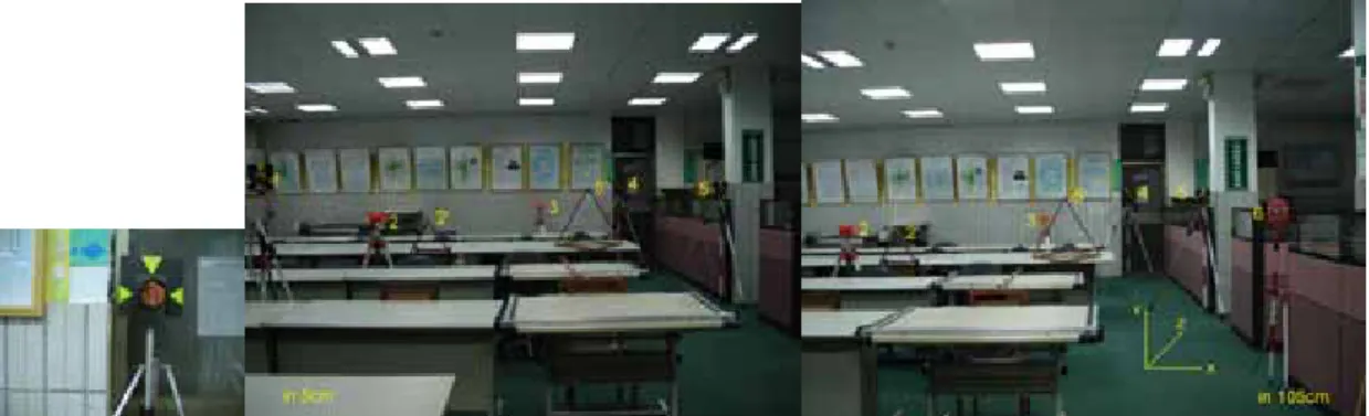
First, we marked the objects which were dispersed in the scene as shown in
Figure 8. We used phototheodolite to measure the absolute coordinates of the
markers as shown in Table 2. In Figure 8, we selected and labeled eight points in the
scene. In Table 2, we showed the absolute coordinates of each point.
Figure 8. The marker was dispersed in the scene. (a) The marker for phototheodolite
to measure the distance. (b) The scene we toke when the camera attached to slide
plate with bar in 5 cm. (c) The scene we toke when the camera attached to slide plate
with bar in 105 cm.
Table 2. The absolute coordinates of the markers.
coordinate x(m) z(m) y(m)
1 -2.131 3.724 1.484
2 -2.006 6.398 1.115
2' -1.416 6.398 1.115
3 0 10.631 1.118
5' 1.436 6.977 1.161
4 1.519 11.054 1.502
5 2.056 6.977 1.118
6 1.998 4.224 1.286
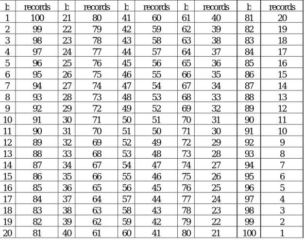
Second, we increased b value in regularity between one and one-hundred
centimeter to take picture for analysis. We took one hundred and one pictures in
each run. The numbers of the data records in b value are shown in Table 3.
Table 3. The numbers of the data records in different b value.
b records b records b records b records b records
1 100 21 80 41 60 61 40 81 20
2 99 22 79 42 59 62 39 82 19
3 98 23 78 43 58 63 38 83 18
4 97 24 77 44 57 64 37 84 17
5 96 25 76 45 56 65 36 85 16
6 95 26 75 46 55 66 35 86 15
7 94 27 74 47 54 67 34 87 14
8 93 28 73 48 53 68 33 88 13
9 92 29 72 49 52 69 32 89 12
10 91 30 71 50 51 70 31 90 11
11 90 31 70 51 50 71 30 91 10
12 89 32 69 52 49 72 29 92 9
13 88 33 68 53 48 73 28 93 8
14 87 34 67 54 47 74 27 94 7
15 86 35 66 55 46 75 26 95 6
16 85 36 65 56 45 76 25 96 5
17 84 37 64 57 44 77 24 97 4
18 83 38 63 58 43 78 23 98 3
19 82 39 62 59 42 79 22 99 2
20 81 40 61 60 41 80 21 100 1
For comparison, we used two kinds of digital cameras to offer the different
resolutions in our experiment. We also selected a number of different outdoor and
indoor scenes for evaluation.
As to how to train, validate and test we will talk them in the latter section.
4.3 Data Analysis
In our experimental design for each run we can get ninety-six pictures in
different baseline at least, so we can calculate b value from one to ninety-five
centimeter. Count of the data records in different b value is shown in Table 3. On
the other hand, we care very much about the confidence of the analysis, so we use b
value within one to eighty-one for data analysis. That means the data records less
than twenty will be omitted in analysis.
When we take pictures during the experiment, we must make sure that the bar
and slide plate are both horizontal. So we omitted the vertical coordinate and read
the horizontal coordinate of the corresponding point which we marked. We
calculated d values between two corresponding points as shown in Appendix A.1 for
Pentax and Appendix A.2 for Casio. The labels in the Appendix A.1 and A.2 are
shown in Figure 8 and illustrated as follows.
B value is the length of baseline between two shots. The unit of b value is
centimeter.
Z value is the vertical distance between the horizon of marker and camera. The
unit of z value is meter.
D value is the disparity of two corresponding points. The unit of d value is
pixel.
In Appendix A.1 abd A.2 we can see that the data of point 1 and point 6 are not
complete in all b values so we omitted it for analysis too. We left six points with
coordinate known for training and validation to find lineal regression equation.
For comparison we used two cameras with different resolutions, so we need to
normalize the value of disparity between two cameras. As we know in Eq. 2.3, base
line (b) is proportional to disparity (d), so we draw them to observe the relation as
shown in Figure 9.
z=3.724
z=6.398 z=6.398
z=10.631 z=6.977
z=11.054 z=6.977 z=4.224
0.0 50.0 100.0 150.0 200.0 250.0 300.0 350.0 400.0 450.0
1 5 9 13 17 21 25 29 33 37 41 45 49 53 57 61 65 69 73 77 81 85 89 93 97 Base line(cm)
Disparity(pixel)
Figure 9. The disparity with different base line show for each marker.
In Figure 9, we can find there are little differences between two types of cameras
after normalization and base line (b) is almost proportional to disparity (d) and the
slope is decreased with z values. The results is coincide with the Eq. 2.6.
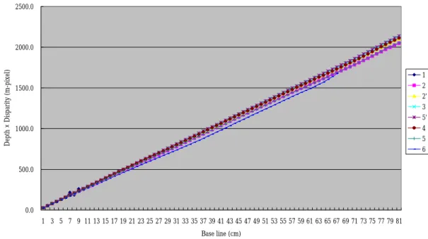
Previously we talked about data selection for analysis, and we left six points with
coordinate known for training and validation to find lineal regression equation. In
Eq. 2.3, base line (b) is proportional to disparity (d), so we can use least square
regression for analysis. In Eq. 2.6, we recalculate z×d for six points as shown in
Appendix A.3, A.4 and made the drawing Figure 10, 11 for for Pentax and Casio
respectively.
0.0 500.0 1000.0 1500.0 2000.0 2500.0
1 3 5 7 9 11 13 15 17 19 21 23 25 27 29 31 33 35 37 39 41 43 45 47 49 51 53 55 57 59 61 63 65 67 69 71 73 75 77 79 81 Base line (cm)
Depth × Disparity (m-pixel)
1 2 2' 3 5' 4 5 6
Figure 10. The relation between z×d and base line for Pentax.
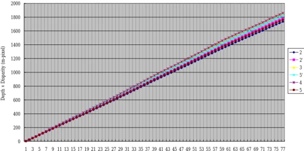
In Figure 11, we can find the lineal relation between b and z×d for each point.
The results are identical with the Eq. 2.7 and the slope is focus of the camera.
0 200 400 600 800 1000 1200 1400 1600 1800 2000
1 3 5 7 9 11 13 15 17 19 21 23 25 27 29 31 33 35 37 39 41 43 45 47 49 51 53 55 57 59 61 63 65 67 69 71 73 75 77 Base line (cm)
Depth × Disparity (m-pixel)
2 2' 3 5' 4 5
Figure 11. The relation between z×d and base line for Casio.
4.4 Calculation of Parameter
In this section, we tried to find out proper regression equation and how many
points we need to train. We also tried to calculate the predicted error rate in
validation sets.
Predicted error rate= | (estimated z - true z)/( true z) | (4-1)
We separated six points into two portions, one of them was called training data
sets and the other called validation data sets. In the training data sets we calculated
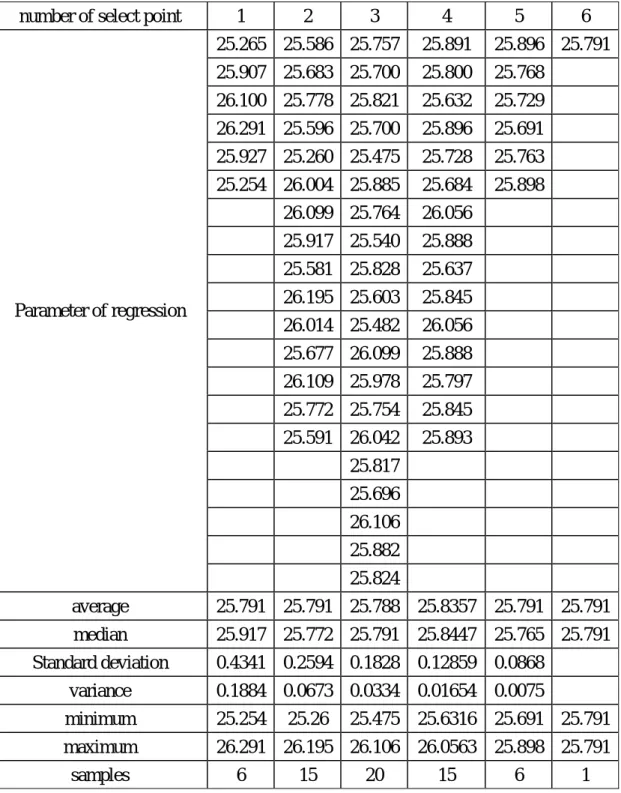
the parameter of regression as shown in Table 4.
In Table 4, we can see that the average numbers of parameters are quite similar
and lay between 25.254 (minimum) and 26.291 (maximum). In Table 5, we used
analysis of variation (ANOVA) to test significance. We found that F value was less
than critical value in 0.05 level of signification, so we accepted the null hypothesis.
It means that the numbers in the training set are not significantly different.
Table 4. Regression analysis with different number of training data sets.
number of select point 1 2 3 4 5 6 25.265 25.586 25.757 25.891 25.896 25.791 25.907 25.683 25.700 25.800 25.768 26.100 25.778 25.821 25.632 25.729 26.291 25.596 25.700 25.896 25.691 25.927 25.260 25.475 25.728 25.763 25.254 26.004 25.885 25.684 25.898 26.099 25.764 26.056 25.917 25.540 25.888 25.581 25.828 25.637 26.195 25.603 25.845 26.014 25.482 26.056 25.677 26.099 25.888 26.109 25.978 25.797 25.772 25.754 25.845 25.591 26.042 25.893 25.817 25.696 26.106 25.882 Parameter of regression
25.824
average 25.791 25.791 25.788 25.8357 25.791 25.791 median 25.917 25.772 25.791 25.8447 25.765 25.791 Standard deviation 0.4341 0.2594 0.1828 0.12859 0.0868
variance 0.1884 0.0673 0.0334 0.01654 0.0075 minimum 25.254 25.26 25.475 25.6316 25.691 25.791 maximum 26.291 26.195 26.106 26.0563 25.898 25.791
samples 6 15 20 15 6 1
Table 5. ANOVA with different number of training data sets.
variables SS df MS F P-value Critical value Between-class 0.024518 5 0.004904 0.100234 0.991678 2.376684
Within-class 2.788551 57 0.048922
sum 2.813069 62
We also calculated different ratio with all selected data as shown in Table 6.
Table 6. Different ratio with different number of training data sets.
point of no. we selected
Parameter of regression
different ratio with all selected
point of no. we selected
Parameter of regression
different ratio with all selected
point of no. we selected
Parameter of regression
different ratio with all selected 5' 26.291 -1.9% 35'4 26.106 -1.2% 2'35'4 26.056 -1.0%
3 26.100 -1.2% 2'35' 26.099 -1.2% 235'4 26.056 -1.0%
4 25.927 -0.5% 2'5'4 26.042 -1.0% 22'5'4 25.896 -0.4%
2' 25.907 -0.5% 2'34 25.978 -0.7% 35'45 25.893 -0.4%
2 25.265 2.0% 235' 25.885 -0.4% 22'35' 25.891 -0.4%
1
5 25.254 2.1% 35'5 25.882 -0.4% 235'5 25.888 -0.4%
35' 26.195 -1.6% 25'4 25.828 -0.1% 2'35'5 25.888 -0.4%
5'4 26.109 -1.2% 5'45 25.824 -0.1% 25'45 25.845 -0.2%
2'5' 26.099 -1.2% 22'5' 25.821 -0.1% 2'5'45 25.845 -0.2%
34 26.014 -0.9% 2'5'5 25.817 -0.1% 22'34 25.800 0.0%
2'3 26.004 -0.8% 234 25.764 0.1% 2'345 25.797 0.0%
2'4 25.917 -0.5% 22'3 25.757 0.1% 22'5'5 25.728 0.2%
25' 25.778 0.1% 2'35 25.754 0.1% 22'45 25.684 0.4%
5'5 25.772 0.1% 22'4 25.700 0.4% 2345 25.637 0.6%
23 25.683 0.4% 22'4 25.700 0.4%
4
22'35 25.632 0.6%
35 25.677 0.4% 2'45 25.696 0.4% 22'35'4 25.898 -0.4%
24 25.596 0.8% 25'5 25.603 0.7% 2'35'45 25.896 -0.4%
45 25.591 0.8% 235 25.540 1.0% 235'45 25.768 0.1%
22' 25.586 0.8% 245 25.482 1.2% 22'35'5 25.763 0.1%
2'5 25.581 0.8% 22'5 25.475 1.2% 22'5'45 25.729 0.2%
2
25 25.260 2.1%
3
5
22'345 25.691 0.4%
Different ratio= ( parameter with training data sets - parameter with all data)
/( parameter with all data) (4-2)
In Table 6, we can find that parameter different ratios all lie in between -2% and
2%.
We put point 2, 3, 4, 5 into training data set and the result of least square
regression in SPSS are shown in Table 7, and drawn in Figure 12.
Table 7. The result of least square regression in SPSS.
camera Unstandardized Coefficients t Sig.
b Std. Error
Pentax 25.637 .009 2888.383 .000
Casio 24.028 .020 1179.23 .000
Figure 12. The result of least square regression in SPSS (a) for Pentax (b) for Casio In Table 9, we can find the regression equation as follows, and we use it to
estimate the object distance. For Pentax, the regression equation is zd=25.637×b,
and focus is 25.637. For Casio, the regression equation is zd=24.028×b, and focus is
24.028.
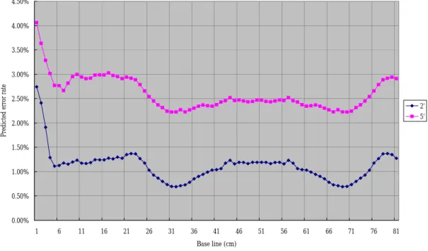
And we put the other point 2' and 5' into validation data sets to predict the depth
of the points and calculate the predicted error rate as shown in Table 8. In Figure 13,
we can seen the variation of the predicted error rate with different b value.
Predicted error rate= | (Predicted value- True value)/ (True value) | (4-3)
Table 8. Predicted error rate with 4 points training set.
No. of point 2 2' 3 5' 4 5
Average of predicted value 6.479 6.323 10.401 6.790 10.905 7.068 True value 6.398 6.398 10.631 6.977 11.054 6.977 Predicted error rate 1.3% 1.2% 2.2% 2.7% 1.3% 1.3%
In Table 8, we can find the predicted error rate between training and validation
are quite near.
0.00%
0.50%
1.00%
1.50%
2.00%
2.50%
3.00%
3.50%
4.00%
4.50%
1 6 11 16 21 26 31 36 41 46 51 56 61 66 71 76 81
Base line (cm)
Predicted error rate
2' 5'
Figure 13. The predicted value with respects to b value for 4 points training set.
We put point 2, 3 and 5 in training set and put point 2', 4 and 5' in validation set
recalculate predicted error rate for each b value as shown in Figure 14.
0.00%
0.50%
1.00%
1.50%
2.00%
2.50%
3.00%
3.50%
4.00%
4.50%
5.00%
1 6 11 16 21 26 31 36 41 46 51 56 61 66 71 76 81
Base line (cm)
Predicted erroe rate
2' 4 5'
Figure 14. The predicted value with respects to b value for 3 points training set.
0.22000 0.23000 0.24000 0.25000 0.26000 0.27000 0.28000 0.29000 0.30000 0.31000 0.32000 0.33000 0.34000 0.35000 0.36000 0.37000 0.38000 0.39000 0.40000 0.41000 0.42000 0.43000 0.44000 0.45000
1 6 11 16 21 26 31 36 41 46 51 56 61 66 71 76 81
Base line b/d
2_b/d_6.398 2'_b/d_6.398 3_b/d_10.631 5'_b/d_6.977 4_b/d_11.054 5_b/d_6.977