朗之萬方程式在蛋白質瞬間增量模型之應用

(1)

國立臺灣大學生命科學院生化科學研究所碩士論文

Graduate Institute of Biochemical Sciences College of Life Science

National Taiwan University Master Thesis

朗之萬方程式在蛋白質瞬間增量模型之應用 The Langevin approach for protein burst production

顏兆銘 Chao-Ming Yen

指導教授：陳水田博士許昭萍博士 Advisor: Shui-Tein Chen, Ph.D.

Chao-Ping Hsu, Ph.D.

中華民國 102 年 7 月

July, 2013

(2)

臣。

指導的框授許讓我這都感謝江蘇問完 Ram 大的謝你

能夠完成這因為有他們導教授陳水田框架，以系統許昭萍老師我得以用數學都歸功於許老謝許老師理論蘇峰和顏清哲完一些怪問題 mesh Anna 的啟發，解決你們。

這篇論文，

們無私的付田老師。陳統的角度去

，許老師願學模型一窺老師願意耐論物化實驗哲，謝謝你題後又帶著 avajjala 在 I

決了我在進

首先我想感付出和支持陳老師鼓勵我去看待複雜的願意讓一位沒窺生物系統的

耐心地解釋基驗室裡生物組

你們總是適時著滿意的答 IEEE Comm 進行電腦模擬

誌謝

感謝我的父

，使我得以我們自主思的生命現象沒有理論背的奧妙。雖然

基本觀念並組的成員們

時地為我解答案離開。

munications 擬時所碰到

父母，他們以專心完成思考，讓我象。再來我背景的學生然相處不到並同時包容們：陳奕丞、

解惑；尤其最後，我想 s Letters 上到的問題，

是這篇論文學業。然後有機會跳脫想感謝我的來參與電腦到一年，但我我的鑽牛角 Surendhar 是清哲學長想謝謝 Am 上發表的論文

進而催生了

文最大的幕後我想感謝脫以往微觀的另一位指腦模擬的研我學到了很角尖。然後 Reddy Che 長，總是能

mine Maare 文，它給了了這篇論文

幕後功謝我的觀生化指導教研究，

很多，

後我想 epyala、

能讓我 ef 和了我莫文，謝

(3)

中文摘要

基因的表達中牽涉了許多隨機的化學分子碰撞與交互作用。而這些隨機的特性反映在蛋白質上，造成量的不確定性且上下波動，類似雜訊。這些雜訊在近年的研究被證實對生物系統有絕對的重要性，舉凡幹細胞分化、或者噬菌體在裂解 (lytic)與溶源(lysogenic)間的決策行為，都與是生物體利用雜訊的現象。而這些基因雜訊的研究皆可以透過數學模型，或是利用電腦模擬隨機過程來獲得可靠的結論。在本論文中，我們利用 Gillespie 演算法來模擬最近提出的蛋白質瞬間增量(burst production)的現象，然後我們利用統計理論推導出朗之萬方程式(Langevin equation) 逼近 Gillespie 演算法所需要的正確雜訊強度。我們發現在蛋白質瞬間增量的情況

下，朗之萬方程式的雜訊強度是沒有瞬間增量的 2倍。這個結果讓我們在研究基

因調控網路中的雜訊行為時，可以用朗之萬方程式來取代原本的 Gillespie 演算法，

並利用朗之萬方程式可以分離雜訊的特點，去追縱調控網路中各個基因對雜訊的貢獻。

關鍵字：基因雜訊、Gillespie 演算法、朗之萬方程式、burst production、基因調控網路

(4)

ABSTRACT

The gene expression is inherently stochastic, and can be characterized by the distribution of protein levels in individual cells. This stochasticity has been discussed analytically and modeled in stochastic process. In this thesis, we model the recently observed burst effect in protein production and use the Gillespie algorithm for simulation. Later, we derive the corresponding Langevin equation mathematically, and we found that the noise size in burst case is 2 times of non-burst case. Hence we propose a numerical Langevin approach based on stochastic process for gene regulatory network modeling. This approach is capable of describing the burst effect, and it produces the same noise as the traditional Gillespie algorithm, which is an exact realization of the master equation. Furthermore, since it is possible to partition the noise in Langevin equation, this approach has an advantage of studying the noise behavior in specific gene regulatory network.

(5)

LIST OF FIGURES

Figure 2-1 One-dimensional random walk with discretized state. ... 5

Figure 3-1 Three stochastic trajectories generated by Gillespie SSA. ... 16

Figure 3-2 The steady state distribution of reactant species S in Eq.(3.19). ... 17

Figure 3-3 Comparison of the Gillespie algorithm and the Langevin equation. ... 21

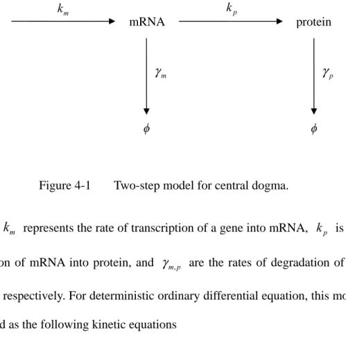
Figure 4-1 Two-step model for central dogma. ... 29

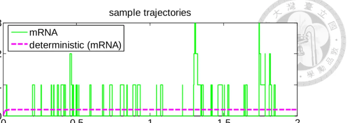
Figure 4-2 A sample stochastic trajectory of mRNA (top) and protein (bottom). Shown are stochastic trajectories simulated by Gillespie algorithm with parameters listed in Table 4-1. ... 34

Figure 4-3 Steady state distribution of mRNA in single expression model. ... 35

Figure 4-4 Steady state distribution of protein in single expression model. ... 35

Figure 4-5 Approximating Gillespie algorithm with different size of dt in Langevin. .. 38

Figure 4-6 Langevin trajectory for mRNA (green) with different size of dt, compared to the stochastic trajectory of Gillespie (red) and deterministic ODE solution (dashed line). Parameters used in simulation are listed in Table 4-1 of section 4.1. ... 39

Figure 4-7 Langevin trajectories for protein with different size of dt, compared to the trajectory of Gillespie algorithm and deterministic ODE solution. Parameters used in simulation are listed in Table 4-1 of section 4.1. ... 40 Figure 4-8 The errors of Langevin simulation as compared to analytical results,

different combination of parameters (km , dt) is used for scanning. Shown are error in Mean (upper panels) and in Fano factor (lower panels) for traditional Langevin (Eq. (4.9)). The error are the difference between the

(8)

statistic values of proteins from 10,000 trajectories as compared to analytical results at steady state (Eq. (4.8) in section 4.1). ... 42 Figure 4-9 Approximating Gillespie algorithm with (km = 0.006, dt = 250) in Langevin equation. (M denotes “mean” and F denotes “Fano factor,” respectively) ... 43 Figure 4-10 Particle number distribution in mRNA (left) and Protein (right) at a higher expression rate with parameters (km = 0.08, dt = 50), the figure shows that Langevin approximation can be valid in a higher expression case. ... 44 Figure 5-1 Transformation of the two-step gene expression model into the translational burst model. ... 47 Figure 5-2 Translational burst production model for central dogma. ... 50 Figure 5-3 Sample trajectories of Gillespie in two-step model and burst model. The

parameters used in simulation are listed in Table 4-1 of section4.1. ... 52 Figure 5-4 Steady state distributions of protein in two-step model and in burst model.

Shown are distributions from 10,000 trajectories simulated with the parameters listed in Table 4-1 of section 4.1. The simulation results of both models in Gillespie algorithm are quite the same. ... 52 Figure 5-5 Illustrated queuing problem ... 54 Figure 5-6 A schematic description for two-step model (left) or a bursting one-step

model (right), and for Gillespie algorithm (upper panels) and their corresponding Langevin equation (lower panels)... 64 Figure 5-7 A sample trajectory for Langevin simulation in burst model. The parameters used in simulation are listed in Table 4-1 of section4.1. The time step used in simulation is 150 sec. ... 65 Figure 5-8 Steady state distribution of protein in different simulation approaches.

(9)

parameters listed in Table 4-1 of section 4.1. The time step used in both Langevin forms is 150 sec. ... 66 Figure 5-9 Comparison of different error levels in two different Langevin forms.

Shown are error in Mean (upper panels) and in Fano factor (lower panels) for traditional Langevin (Eq. (3.37) in section 3.3.2 or Eq. (4.9) in section 4.2, panels to the left) and the Burst-Langevin (Eq. (5.32) in section 5.2.2, panels to the right) in simulating a single gene expression model with the parameters listed in Table 4-1. The error are the difference between the statistic values of proteins from 10,000 trajectories as compared to analytical results at steady state (Eq. (4.8) in section 4.1). ... 67

(10)

LIST OF TABLES

Table 3-1 An intuitive SSA ... 11

Table 3-2 Standard procedures for Gillespie SSA ... 14

Table 3-3 The τ-leap condition ... 24

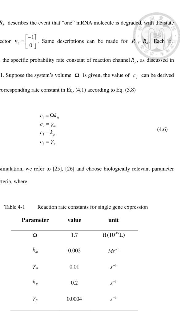
Table 4-1 Reaction rate constants for single gene expression ... 32

Table 4-2 Probability rate constants for single gene expression ... 33

Table 5-1 Statistical quantities derived from Gillespie simulation and analytical Gamma distribution. ... 49

(11)

Chapter 1 Introduction

Gene expression is a series of biochemical reactions, each involves a different degree of randomness. The stochastic fluctuation in gene expression can result in uncertainties of protein concentration, and leads to cell-to-cell variations, or heterogeneities [1]. Moreover, this phenomenon is ubiquitous and has been demonstrated through dual-fluorescence experiments in different biological systems such as E. coli [2], C. elegans [3], and mouse [4]. The gene expression noise can arise from multiple sources [5]. For gene expression level, it could be the different particle numbers of mRNA/protein degradation machinery, or different nucleosome occupancy, or even the different nuclear architecture. For other extrinsic factors, it could be the fluctuation in microenvironment, or different partitioning after cell division, or it could be some pathway-specific propagation, where the intrinsic noise from upstream regulatory gene becomes the extrinsic noise of the downstream gene through regulation [5]-[8]. The noise in gene expression is not just an unwanted effect; instead, it has important functional role in biological system. Since many biochemical processes involves low copy number, this makes cell more susceptible to noise, and it leads to a possibility that heterogeneity in phenotype could be the consequence of different level of fluctuation in genetic network [9].

One of the key functional advantages of noise is the ability to enable probabilistic differentiation of otherwise identical cells. For example, the stochastic mating-type switch in Saccharomyces cerevisiae; the stochastic choice of cell type in asymmetric cell division processes of Drosophila melanogaster [10]; or the fluctuation in Nanog expression of mouse embryonic stem cells, which leads to stochastic cell fate decision [4], [9]. Another noise-driven cellular phenomenon is the stochastic state-switching in

(12)

the context of physiology, development, stress response, cancer and pathogenicity [11].

For example, the switch between lysogenic and lytic state in bacteriophage λ is mediated through the molecular fluctuation of the repressor CI [12].

Cells may determine their fates by playing dice with controlled odds [13]. For example, increasing evidences have shown that cells evolved strategies to control, or to exploit this inherent stochasticity, through the specific architecture of gene regulatory networks (GRN) [1], [5], [9]. Such interactions could include transcriptional regulation and post-translational modifications. For example, the stochastic-state switching systems are often based on positive feedback loops, which amplify the noise and leads to a bimodal distribution in extreme cases; conversely, and negative feedback loops tends to attenuate the noise and narrow the distribution to uniform the cells [14]. Hence cells in differential process tend to maintain the variability and hence prefer the noise-amplifying circuits, while cells in mature state might choose noise-filtering circuits to maintain the stability [9].

As the rapid development of biological technology has provided evidence for stochasticity in gene expression, computer simulation and mathematical analysis on the dynamics can further help to confirm these architecture-dependent noise, or predict the noise of members in the interested gene circuits. To describe the stochasticity in gene expression properly, we need to model the gene networks in the stochastic way. Reliable numerical approaches are needed for generating proper size of noise. Two typical approaches are used in most of gene expression noise related articles: the Gillespie algorithm, and the Langevin equation. Although the Gillespie algorithm provides a more accurate realization of stochastic process, it is not capable of simulating a large network because of the computational cost is high. Conversely, the Langevin equation seems to

(13)

a larger-scale simulation. Moreover, the most important advantage of Langevin equation is the ability the partition the noise (as will be discussed in Section 3.2)

In this thesis, we propose a new formula for describing gene expression noise in the form of Langevin equation, which approximates the Gillespie algorithm in simulating a given single gene expression model that has the translational “bursting”

properties (discussed in chapter 5), and we found the Langevin equation with this new burst production noise is more robust for simulating a single gene expression. Our result provides a better approximation to Gillespie algorithm, compared to the traditional approach discussed in Ref. [19].

(14)

Chapter 2 The Stochastic Process and the Master Equation

A stochastic process, which is a collection of random variables, can often be modeled as a random walk. When applied in the dynamic description, it becomes a sequence of random variables of time. The concept of random walk comes from the famous Brownian motion, which is so unpredictable and full of randomness. To understand the stochastic process, it’s convenient to start from a simple example of one-dimensional random walk [15], [16]. Consider a “drunken” pedestrian that is restricted in one-dimension, and we can discretize the line so that each position equals to a unique state. The set of all possible state is then a state space. In order to make sure it is purely random, suppose the probability of moving forward and backward depends only on the “current state” of the pedestrian; in other words, for current state, the historical behavior has nothing to do with the decision of next move. This memoryless property also called the Markov property, which has been assumed very often in stochastic modeling, and this memoryless random walk also termed a Markov process.

The probability that our drunken pedestrian is in a particular state at some time, can be described as

).

, ( ) ,

| , ( )

,

(S t W S t S t P S t

P _i

i N i

N ⁺^τ ⁼



⁺^τ (2.1)

Here, )P(S_N,t+τ means the probability that the pedestrian is in state S at _N time t+τ, and it depends on where it was previously, orP(S_i,t), multiplied by the

(15)

lasting from t to t+τ . According to the assumption of Markov property, these transition probabilities W are constant functions of time. Taking the continuous time limit, the differential form of Eq. (2.1) becomes

).

( )]

| ( ' )

| ( ' [

) ( )

| ( ' ) ( )

| ( '

1 1

N N

N

N N

S P S S W S

S W

S P S S W S

P S S dt W

dP

+

−

+ +

−

+

−

+

= (2.2)

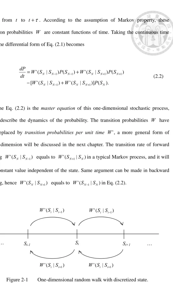
The Eq. (2.2) is the master equation of this one-dimensional stochastic process, which describe the dynamics of the probability. The transition probabilities W have been replaced by transition probabilities per unit time W , a more general form of ' higher dimension will be discussed in the next chapter. The transition rate of forward walking )W'(S_N |S_N₋₁ equals to W'(S_N₊₁|S_N)in a typical Markov process, and it will be a constant value independent of the state. Same argument can be made in backward walking, hence W'(S_N |S_N₊₁) equals to W'(S_N₋₁|S_N)in Eq. (2.2).

Si-1 Si Si+1

… …

)

| ( ' S_i S_i₊₁ W

)

| ( ' S_i S_i₊₁ W

)

| ( ' S_i S_i₋₁ W

)

| (

' S_i S_i₋₁ W

Figure 2-1 One-dimensional random walk with discretized state.

(16)

In Figure 2-1, Si denotes different state, and i is the index of state. This random walk is fully stochastic and can be used to construct a random birth-and-death model to describe the fluctuation in a reactant species. For example, we can substitute our drunken pedestrian with an interested particle, say, mRNA. A step moving forward means one more particle is produced; conversely, a step moving backward means one particle is degraded. We can also introduce more than one species to construct a higher dimensional random walk, and it will be just like a Brownian motion in state space! In other words, in simulating for a biochemical system, the reactions take place according to their reaction probabilities (determined by the corresponding reaction rates), and the

“state” of a system is the particle numbers of all relevant molecules.

In general, it is difficult to solve the master equation analytically in order to realize a stochastic process. Instead, it is usually “solved” in a numerical way by simulating the process with Monte Carlo approach, which collects a large amount of stochastic trajectories and computes the statistics. There are two frequently used numerical approach for describing a stochastic process: the Gillespie stochastic simulation algorithm (Gillespie SSA, or simply Gillespie algorithm) [17]-[19], and the Langevin equation. The Gillespie algorithm is a discrete, and particle number-based stochastic simulation, which can be used to simulate the stochasticity of chemical kinetics in molecular level. Besides, the simulation result of Gillespie algorithm is an exact realization of the master equation, which means there is no any approximation in the result. The Langevin equation is another way to describe stochastic process. It is a differential equation with additional random variables. More details on the Gillespie algorithm and Langevin equation are given in the next chapter.

(17)

Chapter 3 Numerical Approaches for Simulating Stochastic Process

3.1 The Gillespie algorithm

Consider a system of fixed volume Ω contains N different species of reactants, with M different reactions among those reactants, or reaction channels, denotes

) ,..., 1

(j N

R_j = . And assume particle number of each reactant can be expressed as a

continuous function of time X_i(t) (i=1,...,N) . For deterministic process, the dynamics of the system can be described by the following ordinary differential equation (O.D.E.) form:

) ,..., ( ...

) ,..., (

1 1 2 2

1 1 1

N N

N

N N

X X f X

=



(3.1)

For simplification, we use the state vector ))X(t)≡(X₁(t),X₂(t),...,X_N(t to describe the system state at time t. In stochastic process, X_i(t) is actually a random variable. To analyze it, define propensity function aj for reaction channel Rj , which is that

).

,..., 1 ( ) , [ interval time

mal infinitesi next

in the inside

somewhere

occur ill reaction w channel

one that

, (t) given y, probabilit the

) (

M j

dt t t R dt

a

j j

= +

Ω

=

≡ X x

x

(3.2)

(18)

Eq. (3.2) is the fundamental premise for numerically solving the master equation.

Previously it was thought to be an ad hoc assumption for stochastization of the deterministic chemical kinetics [20]. Later it has been proved that the Eq. (3.2) has a rigorous microphysical basis [21].

For each reaction channel Rj, we also need to define the state-change vector v , _j whose ith component is given by

channel.

one

by produced of

number in the

change the

j

i ji

R

X v ≡

(3.3)

Together, Eq. (3.2) and Eq. (3.3) specify the behavior of each reaction channel, the state-change vector v is a fixed vector with integer value, and it’s component is _j usually +1 for production channel, and -1 for degradation channel, while the propensity function aj changes value from time to time accords to the system state x . From previous argument [17], the function aj has mathematical form

).

( )

(x _j _j x

j c h

a = (3.4)

Here, cj is the specific probability rate constant for channel Rj, and cj dt gives the probability that “one” random chosen pair of reactant molecules in Rj will react accordingly in the next infinitesimal time. The unit of cj is the inverse of time, and the value can be determined from traditional reaction constant kj. If the system’s volume Ω is given, cj can be derived from kj by transforming the unit of kj into the same unit of cj. For example, consider two reactant molecular species S and S , and a reaction

(19)

channel R of which _μ S₁ reacts with S₂ to give the product S ₃

. 2

: S₁ S₂ S₃

R_μ + ⎯⎯→^c^μ (3.5)

The reaction channel R_μ was conventionally described by reaction rate constant

kμ in chemical kinetics, more precisely, it’s the average reaction rate per unit volume divided by the product of the average densities of the reactants [17]. Put the definition of cj together, we have

.

/ ₁ ₂

2

1x c x x

x

k_μ = Ω _μ (3.6)

Where x₁ and x₂ represents the molecular concentration of reactant species S₁ and S₂. However, in deterministic formulation we do not consider statistical variance, therefore x₁x₂ = x₁ x₂ , hence it gives the relation

μ.

μ c

k =Ω (3.7)

For other types of reaction channel, this relationship can vary, and we summarize it as following

2 /

; products reaction

2

) (

; products reaction

/

; products reaction

μ μ

μ

φ μ

c k

S

k i c

k S

S

c k S

c k

i k i

i

Ω

≅

→

≠ Ω

=

→ +

=

→

Ω

=

→

(3.8)

(20)

change the value of k of the first three types of reaction after we transfer it to _μ c in _μ stochastic simulation.

The function )h_j(x in Eq. (3.4) is defined to be the number of distinct combinations of Rj reactant molecules available in the state x [19]. For example, the

h for the following types of reaction can be j

2 / ) 1 (

; products reaction

2

; products reaction

1

; products reaction

−

=

→

=

→ +

=

→

=

→

i i j i

k i j k

i

i j i

j

x x h S

S

x h S

φ h

(3.9)

The time-dependent stochastic trajectory can thus be simulated once cj and v are _j given. Here, the evolution of Eq. (3.2) implies that the state vector X(t)is a jump-type Markov process non-negative N-dimensional integer lattice [19], and a traditional way to analyze it is to write it in the form of conditional probability function

}.

) ( iven that

, ) ( { Prob )

,

| ,

(x t x₀ t₀ ≡ X t =x g X t₀ =x₀

P (3.10)

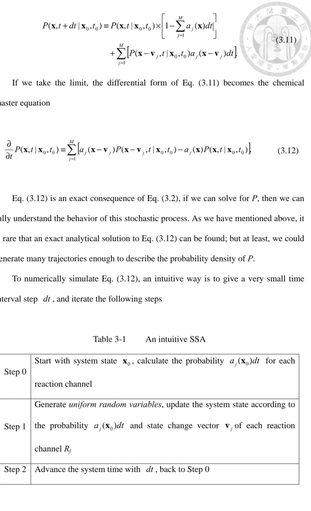
The time-dependent evolution of this conditional probability function can be derived by advance the system with a small time step dt one at a time, so that we can exclude the probability for two or more reactions to occur in dt . Using Eq. (3.2), together with the previous argument [21], the probability of the system being in state x at time t+ can thus be described dt

(21)

[

⁽ ^, ^| ^, ⁾ ⁽ ⁾

]

^.

) ( 1

) ,

| , ( ) ,

| , (

1

0 0

1 0

0 0

0



=

−

− +



 



 −

×

≡ +

M j

j j j

M j

j

dt a

t t P

dt a t

t P t dt t P

v x x

v x

x x

x

(3.11)

If we take the limit, the differential form of Eq. (3.11) becomes the chemical master equation

[

⁽ ⁾ ⁽ ^, ^| ^, ⁾ ⁽ ⁾ ⁽ ^, ^| ^, ⁾

]

^.

) ,

| , (

1

0 0 0

0 0

0



=

−

∂ ≡

∂ ^M

j

j j

j

j P t t a P t t

a t

t

tP x x x v x v x x x x (3.12)

Eq. (3.12) is an exact consequence of Eq. (3.2), if we can solve for P, then we can fully understand the behavior of this stochastic process. As we have mentioned above, it is rare that an exact analytical solution to Eq. (3.12) can be found; but at least, we could generate many trajectories enough to describe the probability density of P.

To numerically simulate Eq. (3.12), an intuitive way is to give a very small time interval step dt , and iterate the following steps

Table 3-1 An intuitive SSA

Step 0

Start with system state x , calculate the probability ₀ a_j(x₀)dt for each reaction channel

Step 1

Generate uniform random variables, update the system state according to the probability a_j(x₀)dt and state change vector v of each reaction _j channel Rj

Step 2 Advance the system time with dt , back to Step 0

(22)

The stochastic simulation result is an exact realization for Eq. (3.12), but the defect is that, since dt is required to be small enough, the probability a_j(x₀)dt that a reaction happens in reaction channel Rj will also be small, it means the computer repeat those three steps frequently, but most of time there’s no reaction happened, this leads to inefficiency of this naive stochastic simulation algorithm, and makes it even unusable if

→0

dt .

Another way to solve this problem of inefficiency is the Gillespie stochastic simulation algorithm, which defines another exact consequence of Eq. (3.2), the next-reaction density functionp(τ, j|x,t) [17], [21], where

reaction.

an be will and , ) ,

[

interval time

mal infinitesi in the

occur will in reaction next

the

, given

y that, probabilit

) ,

| , (

Rj

d t

t

(t) d

t j p

τ τ τ τ

τ

+ + +

Ω

=

≡ X x

x

(3.13)

The τ in Eq. (3.13) stands for the time that elapses without any reaction occurs in the system, and ^p⁽τ^,^j^|^x^,^t⁾^dτ can also be expressed as the product

. ) ( )

,

| ,

(τ ^j ^t ^dτ ^p₀ τ ^a ^dτ

p x = ⋅ _j (3.14)

Here, )^p₀(τ stands for the probability density of this τ , and it can be calculated

by elementary probability argument. Since



= M j

j dt

a

1

)

(x gives the probability that some

reaction will take place in the next dt according to the definition of Eq. (3.2), we can

(23)

divide τ , say, into K equal length subintervals. Let ε denotes the subinterval where ε =τ/K , K is a positive integer, the probability none of the reactions

RM

R ,...,₁ occurs in the first ε subinterval (t, t+ε)is

[

¹ ⁽ ⁾ ⁽ ⁾

]

¹ ⁽ ⁾ ⁽ ⁾^.

1 1

∏

_j^M₌ ⁻^a^j ^x ^ε⁺^o ^ε ⁼ ⁻



^M_j₌ ^a^j ^x ^ε⁺^o ^ε ^(3.15)

Where ^o(ε)describes the probability that more than one reaction occurs in )

,

(t t+ε , and we don’t really need to worry about it since this term can be very small for small ε. The right side of Eq. (3.15) is also the probability that no reaction occurs in the subsequent intervals(t, t+2ε),(t, t+3ε)and so on, since the system state x

remains if no reaction occurs, hence the term



= M j

aj 1

)

(^x ε remains the same. For the rest

of subintervals, using the same argument, we have

. ) ( ) ( 1

) (

1 0

M K

j

j o

a

p 



 



 − +

=



= ε ε

τ ^x ^(3.16)

For K→∞, together with ε =τ/K, Eq. (3.16) is equal to

. ) ( exp

) (

1

0 



 



−

=



= M j

aj

p τ ^xτ ^(3.17)

Hence, after plugging Eq. (3.17) into Eq. (3.14), it becomes

(24)

).

,..., 1

; 0

(

) ( exp

) ( ) ,

| , (

1

M j

a a

t j p

M k

k j

=

∞

<

≤



 



−

=



=

τ

τ ^x ^x ^x

(3.18)

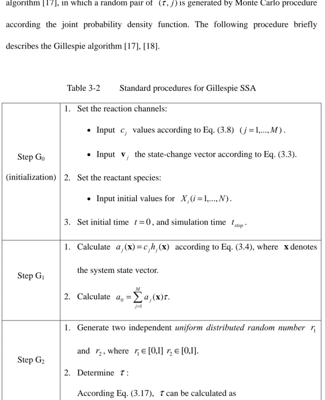
The Eq. (3.18) provides the fundamental basis for Gillespie stochastic simulation algorithm [17], in which a random pair of (τ, j)is generated by Monte Carlo procedure according the joint probability density function. The following procedure briefly describes the Gillespie algorithm [17], [18].

Table 3-2 Standard procedures for Gillespie SSA

Step G₀ (initialization)

1. Set the reaction channels:

• Input c values according to Eq. (3.8) _j (j=1,...,M).

• Input v the state-change vector according to Eq. (3.3). _j 2. Set the reactant species:

• Input initial values for X_i(i=1,...,N). 3. Set initial time t=0, and simulation time t_stop.

Step G1

1. Calculate a_j(x)=c_jh_j(x) according to Eq. (3.4), where x denotes the system state vector.

2. Calculate ( ) .

1

0



=

= ^M

j

aj

a ^xτ

Step G₂

1. Generate two independent uniform distributed random number r₁ and r₂, where r₁∈[0,1] r₂∈[0,1].

2. Determine τ^:

τ

(25)

1).

1 ln(

1

0 r

= a τ

3. Determine the reaction channel R in which the reaction happens: _μ

Take _μ so that .

1 0 2 1

1



=

−

=

≤

< ^μ

μ

j j j

j ra a

a

Step G3

1. Update the simulation time τ.

+

= t t

2. Update the system state according to R _μ

μ. v x

x= +

3. If t>t_stop, or if no more reactants left (all h_μ =0), terminate the simulation; otherwise, return to Step G1.

Here, we use a simple example to demonstrate the Gillespie algorithm. Consider a simple birth-and-death model for a species S , where

.

: :

2 1

φ φ

⎯→

⎯

⎯→

⎯

c c

S R

(3.19)

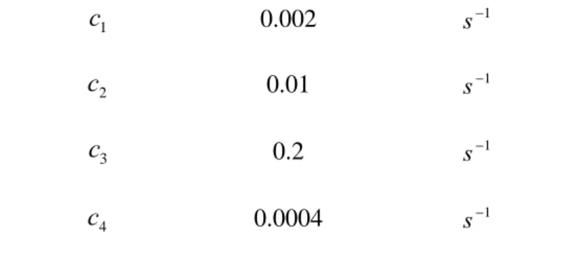
Reaction channel R₁ describes a zero order constant production of species S , and R₂ describes a first order degradation of S ; c₁, c ₂ is dimensionless probability rate constant, as defined in Eq. (3.8).

For conventional understanding in kinetic description, the ordinary differential equation form of this model will be

(26)

2 .

1 k x

dt k

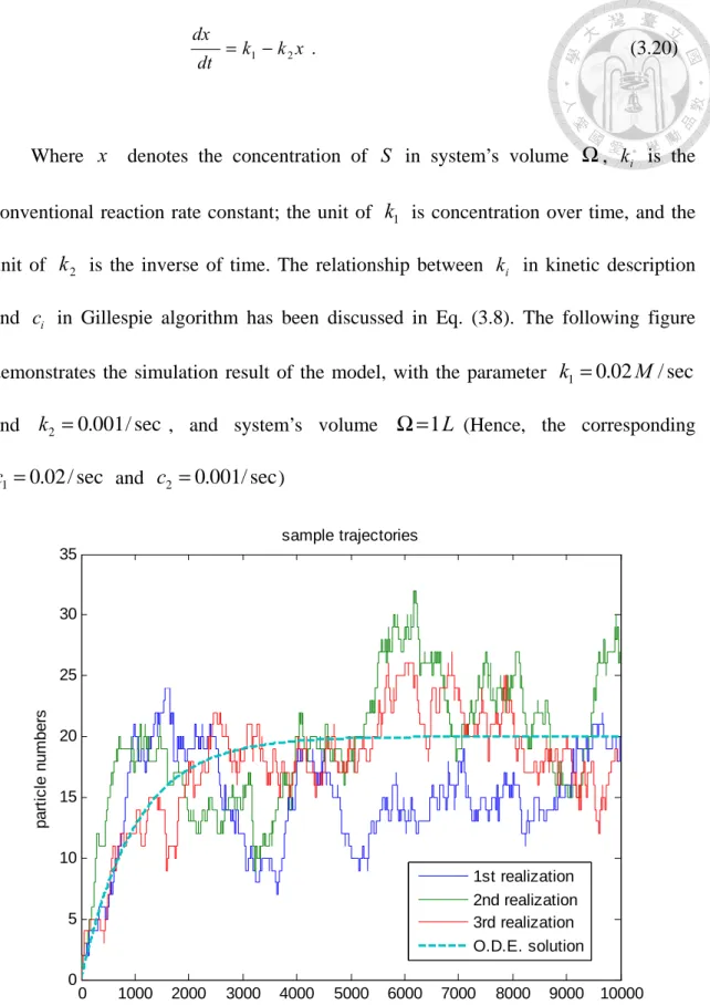
dx = − (3.20)

Where x denotes the concentration of S in system’s volume Ω^, k is the i

conventional reaction rate constant; the unit of k₁ is concentration over time, and the unit of k₂ is the inverse of time. The relationship between k in kinetic description _i and c in Gillespie algorithm has been discussed in Eq. (3.8). The following figure _i demonstrates the simulation result of the model, with the parameter k₁=0.02M/sec and k₂ =0.001/sec , and system’s volume Ω=1L (Hence, the corresponding

sec / 02 .

1=0

c and c₂ =0.001/sec)

Figure 3-1 Three stochastic trajectories generated by Gillespie SSA.

0 1000 2000 3000 4000 5000 6000 7000 8000 9000 10000 0

5 10 15 20 25 30 35

sample trajectories

time(sec)

particle numbers

1st realization 2nd realization 3rd realization O.D.E. solution

(27)

Three trajectories are shown in the Figure 3-1, which are generated by repeating Gillespie algorithm three times, using the birth-and-death model in Eq. (3.19), with parameters described in text. The dashed line represent the analytical solution of Eq.

(3.20), which is a continuous function with mathematical form )

1 ( )

( )

( ²

2

1 e kt

k t k x t

X =Ω =Ω − ⁻ . The capital X denotes the particle number of species

S , and the vertical axis shows the discrete particle number of species S . The

Gillespie algorithm is programmed by MATLAB^®.

In order to reconstruct the probability space of X(t), a large quantities of trajectories should be made. Here, since we are interested in the steady state X , we ^* take value of each trajectory at the end of simulation time (10,000 sec in this case) and analyze statistics of the distribution.

5 10 15 20 25 30 35 40

0 0.02 0.04 0.06 0.08 0.1 0.12 0.14 0.16 0.18

Steady state distribution

particle number

probability

mean = 20.0788 Var = 19.9798 Fano = 0.99507

(28)

The histogram shown in Figure 3-2 is generated by steady state values(value at 10,000 sec. in this case) of 10,000 trajectories simulated with Gillespie algorithm, using the birth-and-death model described in Eq. (3.19). The statistics is made by collecting the steady state value for each trajectory. The distribution of X has mean = 20.08, ^* variance = 19.98 and the Fano factor(defined as variance/mean) ≅ 1, which represents a Poisson distribution.

3.2 The Langevin equation

The Langevin equation is a stochastic differential equation (S.D.E.), which is an ordinary differential equation with noise terms. Originally, the Langevin equation was used to describe Brownian motion, the random movement of a particle resulting from random collision in the solution. The general mathematical form of Langevin equation can be described by

).

, )

(x x t

f

x= +η( (3.21)

Where x is a random variable which varies with time, and f(x) is conventional ordinary differential equation, describing the deterministic time-dependent behavior of

x . In mechanical approach of, f(x) is the sum of "regular forces" acting on the particle while x is velocity of the particle.

The noise term _η is added to make the deterministic equation become stochastic, and _η satisfies the following conditions:

(29)

. 0 )

, =

( tx

η (3.22)

. ( ) ( ) , )

, ( + = )

( η τ δ τ

η ^x ^t ^x ^t ^q ^x (3.23)

Here, δ⁽τ₎ denotes the Dirac delta function and q( x) is an unknown noise-generating function dependent on x, the autocorrelation function of noise equals

τ) δ⁽ )

q(x according to Eq. (3.23) . The first condition is that ensemble average of the noise term equals to zero, hence if we take ensemble average of Eq. (3.21), it equals to the ensemble average of the one with only deterministic part. The second condition describes Markov property, in other words, the noise density of different step is independent of time.

For numerically simulation of Langevin equation, according to [22], the Euler–Maruyama method can be applied. Consider a standard Brownian motion (or standard Wiener process), where a random variable W(t) defined over time interval

] , 0

[ T and depends continuously on time, satisfies the following conditions:

1. W(0)=0 (with probability equals 1)

2. For [0≤s<t<T], W(t)−W(s)~ t−sN(0,1) which means the increment of this stochastic process comes from a normal distribution with mean zero and variance t− , s N⁽⁰^,¹⁾ denotes the unit normal distribution.

3. For [0≤s<t<u<v<T] , the increments W(t)−W(s) and W(u)−W(v) are independent.

The stochastic integral of Eq. (3.21) will be the solution to the stochastic trajectory

(30)

].

, 0 [ ) ( )) ( ( ))

( ( )

(

0 0

0 f x s ds x s dW s t T

x t x

t t

∈ +

+

=

 

^η ^(3.24)

Here, )x₀ =x(0 is the initial condition, the first integral on the right side describes the historical trajectory of the deterministic part, and the second one describes the historical trajectory of the stochastic part. The differential equation form of Eq. (3.24) equals

].

, 0 [ , ) 0 ( ) ( )) ( ( )) ( ( )

(t f x t dt x t dW t x x₀ t T

dx = +η = ∈ (3.25)

To numerically simulate Eq. (3.24), we discretize the interval into L parts. Let L

T t= /

Δ for some positive integer L , and let τ_i =iΔt . The Euler–Maruyama method takes the form

).

,..., 1 (

)) ( ) ( ))(

( ( )) ( ( ) ( )

( ₁ ₁ ₁ ₁

L i

W W

x t x

f x

x _i _i _i _i _i _i

=

− +

Δ +

= τ₋ τ ₋ η τ₋ τ τ₋

τ (3.26)

If we take η ≡0, Eq. (3.26) simply reduced to x(τ_i)=x(τ_i₋₁)+ f(x(τ_i₋₁))Δt^{, and} it’s the form of Euler’s method. In other words, the fundamental concept of Euler–Maruyama method is from Euler’s method, where we use the present step to calculate the increment, and then proceed to the next step according to the increment.

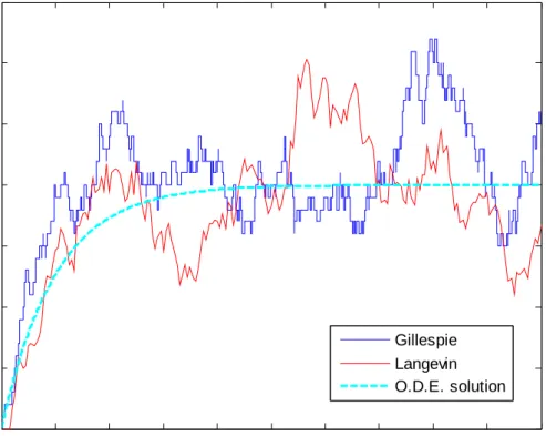
The following figure (Figure 3-3) shows numerical result of the Langevin equation (red), using the same model described in Eq. (3.19) and the same parameter set, compared to the result of the Gillespie algorithm (blue). We note that the Langevin equation takes continuous value, while the Gillespie algorithm displays the discrete

(31)

number of molecular particle. This problem can be bypassed if we further divided particle number with system’s volume, and use the “concentration” to show the result;

or if the system contains large quantity of particle number, the difference between discreteness and continuity could be sew up.

If we take away the noise term in Langevin equation, the Langevin trajectory (red line) in Figure 3-3 will exactly be the same as the trajectory of deterministic O.D.E.

solution (dashed line).

Figure 3-3 Comparison of the Gillespie algorithm and the Langevin equation.

A comparison for the trajectories derived from the Gillespie algorithm (blue line), the Langevin equation (red line), and the corresponding trajectory from the deterministic kinetics (dashed line in cyan).

0 1000 2000 3000 4000 5000 6000 7000 8000 9000 10000 0

5 10 15 20 25 30 35

sample trajectories

time(sec)

particle numbers

Gillespie Langevin O.D.E. solution

(32)

3.3 Approximation of Gillespie algorithm with the Langevin equation

At first glance, the Langevin equation seems to be artificial, since one can simply manipulate the noise term to generate different noise strength. Despite the fact that one can arbitrarily tune the noise, the best thing of Langevin is the ability to separate the deterministic and the stochastic part, and it will become very useful for tracking noise source. Since the Gillespie algorithm is an exact realization of chemical master equation [17], [18], we might ask what is the proper noise size for the corresponding Langevin equation, under the same stochastic model? Before answering this question, we must first realize that these two stochastic approaches are different in nature. First, for simulation aspect, the way of describing the history axis is different. In Gillespie, the history axis of a species in the system is described in different size of waiting time (Eq.

(3.13)). In Langevin, the history axis of every species is segmented into a uniform infinitesimal time interval dt (Eq. (3.25) and Eq. (3.26)), and the evolution of system is described by repeating this dt snapshot. Second, the Gillespie algorithm describe the discrete nature in molecular level, the reactants change numbers according to the reaction channels and the corresponding state change vectors (Eq. (3.3)), while the Langevin equation is a continuous function. Hence, if we want to make the Langevin equation “looks like” the Gillespie algorithm, the difference mentioned above must be overcome. According to the argument of Daniel T. Gillespie in [19], the Gillespie algorithm can be approximated by the Langevin equation, if dt in the Langevin equation satisfies the following two conditions.

(33)

3.3.1 Condition 1: The tau-leaping condition in Gillespie algorithm

For a typical realization of Gillespie algorithm, if we could divide the system’s history axis into a set of contiguous subintervals in such a way that we could forego determine how many times each reaction channel fires in each subinterval, then it’s conceivable to “leap” the history axis with these subintervals. This strategy is originally an acceleration approach for Gillespie algorithm, which is called the τ-leap method [23].

By notations of previous section, suppose the system’s state X(t) at the current time t is denoted as x . Let _t K xj( t,τ) (τ >0) defined as following

).

,..., 1 ( ) , [ interval me

ti

in the fire will channel

reaction e

th

, ) ( given times,

of number the

) , (

M j

t t

R

t K

j t

j

= +

=

≡

τ

τ ^X ^x

x

(3.27)

The number of reactant species S at time _i t+τ can then be expressed as

).

,..., 1 ( ) , ( )

( ) (

1

N i

v K

t X t

X

M j

ji t j i

i + = +



=

τ

τ ^x (3.28)

The second term on the right side of Eq. (3.28) means the summation of changes from each reaction channel, and v denotes the ith component in state change vector _ji

v (Eq. (3.3)). Under this construction, j K xj( t,τ) is a random variable, and it’s difficult to compute K xj( t,τ) just like it’s hard to solve the master equation, since every reaction that takes place within τ can change the system state, and hence the propensity functions a_j(x), since it depends on the current system state (Eq. (3.2) and Eq. (3.4)). In other words, every reaction that happens in τ is not independent of each other, the first reaction in τ will leave some “memory” on the history axis and affect

(34)

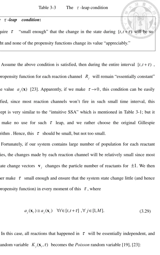
Table 3-3 The τ-leap condition The τ-leap condition:

Require τ “small enough” that the change in the state during [t,t+τ) will be so slight and none of the propensity functions change its value “appreciably.”

Assume the above condition is satisfied, then during the entire interval [t,t+τ) , the propensity function for each reaction channel R will remain “essentially constant” _j at the value a_j(x) [23]. Apparently, if we make τ →0, this condition can be easily satisfied, since most reaction channels won’t fire in such small time interval, this concept is very similar to the “intuitive SSA” which is mentioned in Table 3-1; but it will make no use for such τ leap, and we rather choose the original Gillespie algorithm . Hence, this τ should be small, but not too small.

Fortunately, if our system contains large number of population for each reactant species, the changes made by each reaction channel will be relatively small since most of state change vectors v changes the particle number of reactants for _j ±1^{. We then} further make τ small enough and ensure that the system state change little (and hence the propensity function) in every moment of this τ ^{, where}

].

, 1 [ , ] , [ ' ) ( )

( _' a t t t j M

a_j ^x_t ≅ _j ^x_t ∀ ∈ +τ ∀ ∈ (3.29)

In this case, all reactions that happened in τ will be essentially independent, and the random variable K xj( t,τ) becomes the Poisson random variable [19], [23]:

(35)

).

,..., 1 ( ) ), ( ( )

,

( Poisson a j M

K_j ^x_t τ = _j ^x_t τ = (3.30)

The term Poisson denotes a Poisson random variable, and the mean of )

), ( (aj t τ

Poisson x equals to a xj⁽ t⁾τ . The net effect of the τ-leaping condition allows Eq. (3.28) to be approximated by

).

,..., 1 ( ) ), ( ( )

( ) (

1

N i

v a

Poisson t

X t

X ^M

j

ji t j i

i + = +



=

τ

τ ^x (3.31)

Eq. (3.31) is the τ -leaping method, and it provides a fundamental argument of the existence of such τ . Remember it’s just an approximation; it means that the error could become large if the τ is too big, and the result will be close to the exact realization of Gillespie algorithm, if the τ is small enough.

3.3.2 Condition 2: Approximation with a normal random variable

Suppose we could find a set of τ which satisfies the tau-leaping condition, the Eq.

(3.31) can be used to substitute the original Gillespie algorithm. If, for this set of τ ^, there exist a subset which further satisfies the condition where

].

, 1 [ , 1 ) ( ) ), (

(a a j M

Poisson _j ^x_t τ = _j ^x_t τ >> ∀ ∈ (3.32)

In other words, for every reaction channel, the average firing times within τ

(36)

events, and the random variables of Poisson distribution are integers by definition; the condition in Eq. (3.32) provides a bridge for connecting the discrete Gillespie algorithm to continuous Langevin equation, because when mean is large, a discrete Poisson random variable can be approximated by a normal random variable, with same mean and variance [19], [23]. Where

, 1 ) ( for ) ) ( , ) ( ( )

), (

(aj t τ ≈Normal aj t τ aj t τ aj t τ >>

Poisson x x x x (3.33)

Here, we use the term Normal to denote a normal distributed random variable.

Under the condition of Eq. (3.32), the τ -leaping form of Eq. (3.31) becomes

).

,..., 1 ( ) ) ( , ) ( ( )

( ) (

1

N i

v a

a Normal t

X t

X ^M

j

ji t j t j i

i + = +



=

τ τ

τ ^x ^x (3.34)

Notice that the increment of X_i(t) is now taking continuous random variable from normal distribution. By linear combination theorem for normal random variables

).

1 , 0 ( )

,

(m ² m Normal

Normal σ = +σ (3.35)

Eq. (3.34) now becomes:

).

,..., 1 ( ) 1 , 0 ( ) ( )

( )

( ) (

1 1

N i

N a

v a

v t

X t

X ^M

j ji j t j

M

j ji j t

i

i + = +



+



=

τ τ

τ ^x ^x (3.36)

(37)

Where N_j(0,1) denotes the independent unit normal random variable for each reaction channel R . Consider a time step _j τ which can satisfy both conditions, and substitute this τ with the notation dt , we then rewrite the Eq. (3.36) into

).

,..., 1 ( ) 1 , 0 ( ) ( )

( )

( ) (

1 1

N i

N dt a

v dt a v t

X dt t

X ^M

j ji j t j

M

j ji j t

i

i + = +



+



=

x

x (3.37)

Eq. (3.37) is the working form for numerical simulation of Langevin equation, which approximates the corresponding Gillespie algorithm. The differential form of Eq.

(3.37) equals to

), ( )) ( ( ))

( ) (

(

1 1

t t a v t

a dt v

t dX

j M

j ji j

M

j ji j

i =



+



Γ

=

X

X (3.38)

where Γ_j(t) are temporally uncorrelated, statistical independent Gaussian white noise.

Eq. (3.38) is exactly a Langevin equation, and the noise term is consistent with the properties described in Eq. (3.22) and Eq. (3.23). Up to this step, we have already transform the original Gillespie algorithm (which stands for the exact simulation of master equation) into the corresponding Langevin equation. The second term of Eq.

(3.38) can be regarded as the noise extracted from the master equation, if we eliminate this term, Eq. (3.38) simply go back to deterministic ordinary differential equation.

The second condition requires τ in Langevin equation being “large enough” to ensure that aj(^x)τ >>1, so normal distribution can approximate well to Poisson