針對安全攸關之嵌入式即時系統的異質性資訊融合

(1)

↵À˙c'x˚_«⌦xb«⌦Â↵x˚

©Î÷á

Department of Computer Science and Information Engineering College of Electrical Engineering and Computer Science

National Taiwan University Master Thesis

› âh8‹KLe✏sB˚qÑpÍ'«⌦ç

Heterogeneous Sensing Fusion for Safety Critical Embedded Real-time Systems

‰ s

Chun-Wei Ku

⌥ Yà⇢Ω ⌥ ZÎ

Advisor: Chi-Sheng Shih, Ph.D.

-Ô⌘↵ 107 t 1

January, 2018

(2)

(3)

Ù Ù Ù

àÿ ÍÒÔÂå⇣⇡ ˝©Î÷á à ´äÑ∫itÜÑ

Y Â j4ì⌘ÔÂå⇣⇡«÷á⇥

ñH⌘Å ⌘Ñ⌥ +Ω ⌥Yà YàitÜY ⌘

ÇU↵~OL ÇUÂ¥9Ñπ✏ª ⇤⌥÷ Ê/k©⌘å⇣÷

áÑ 'kK⇥

çÜ^8 Elastic Team Ñ x⌘Â ‚˘¥ZÎ ˘¥=

/ º–õ1⇢˙p _ Elastic Team ⇡µBìÑj4 (∞

Î÷áa‹B å x⌘Ñ ÷=/ÔÂì⌘û-¿|˙1⇢Û’⇥

ÑÅ 1⇢v÷ÊW§Ñ x⌘Â ⌘Ñ§À ÷6v⇠ﬂ

⌅ ¯ F/( #ÑSÔ⌦M2 wv M2=‘ ↵∫hÍ

÷‹ ’õ⇢Ü⇥

å ⌘ÑΩΩå y⌘Ñ Ô/ å⌦≤ Ô

Â⌃)bm}}ﬁ1y⌘Ñÿ˙⇥

ç!Ñ @ k©N⌘Ñ∫ `⌘⇥

⌫, ✏, 2017

‰ s

(4)

X X XÅ Å Å

˛ 1⇢ çÑü‡˝/˙Íº’€Ñè˝ /’€B⌃√⇥

H2’€©˚qs/∫Ü©’€⇧ÑL âh |UÑ˚q⇥v

- (H2’€©˚q· %^ ©˚q/ ↵ÕÅÑpL

Û 1⇢Ñv Ëºd⇥ ˚fñ∫ ˜T IT˝/—tÜ8

´…(( %^ ©˚q⌦ÑÄS⇥1ºw›‚u,K˜TåIT

Ñ˘<^8⇥¥ ‡d⌘⌘ ≈(qœ ,h( %^ ©˚

q⌦⇥¯⇤ºÍ( ↵qœ ,hÑ˚q ⌘⌘–˙Ü ↵ÔÂP

ñŒƒ Ñqœ ,hK˚q⇥d˚q✏NP ñŒƒ

Ñqœ ,h T0‘( ↵qœ ,hÑ˚qÙ}Ññ∫á⇥

B ⌘⌘_MNÜi‘u,B§çÑ_á⇥ å 1ºLe✏sB˚

qÑKó˝õ/ PÑ ‡d⌘⌘_≈ † ,h«⌦t π’⇥

(Ü⌘⌘–˙Ñ˚qKå ¯⇤º≈( ↵qœ ,hÑ˚qÔ

Â–GÛ⇢10%Ññ∫á⇥

‹

‹uuuWWW- pÍ'«⌦ç pÍ'qœ ,h˚q %^ ©

˚q i‘u,

(5)

Abstract

Nowadays, the bulk of these road collisions is caused by human unawareness or distraction. Since the most important thing is your safety and the safety of others, ADAS is developed to support enhanced vehicle system for safety and better driving. AEBS as an important part of the ADAS has become a hot research topic. Computer vision, together with Radar and Lidar, is at the forefront of technologies that enable the evolution of AEBS. Since the cost of long range radar and lidar is very high, we want to use camera-based system to construct AEBS. Instead of using a single monocular camera, we propose a heterogeneous camera-based system to use sensor fusion to combine the strengths of all the difference FoV cameras. Also, We use a heuristic false positive removal method to decrease the false positive rate that caused by the sensor fusion method. We optimize the sensor fusion method Because of the the limitation of computing resource on embedded system. As a result, the recall of YOLO can be increased up to 10% through our heterogeneous camera-based system.

Keywords - Heterogeneous Sensing Fusion, Heterogeneous Camera-Based Sytem, Tri-focal camera, AEBS, Object Detection

(6)

List of Figures

1.1 ADAS functions . . . 2

1.2 An example of ADAS sensors. . . 3

1.3 An example of different FoV camera. (a) wide-angle camera. (b) focal length between wide-angle camera and telephoto camera. (c) telephoto camera. . . 4

1.4 An example of true positive, true negative, false positive, false negative . 5 2.1 AEBS-TTC testing . . . 7

2.2 The YOLO detection system . . . 8

2.3 Data (gray rectangles) organized in a R-tree with M = 3, m = 2 . . . 10

2.4 R-tree (with M = 3, m = 2) for the data rectangles of Figure 2.3 . . . 11

2.5 Hilbert curves of order 1, 2 and 3 . . . 12

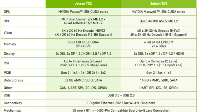
3.1 The ability of NVIDIA Jetson TX1 and TX2 . . . 15

3.2 The architecture of the proposed heterogeneous camera-based system . . 16

4.1 Data flow of the heterogeneous camera-based system. . . 19

4.2 The frame that composed by three different FoV camera and the ROI of each camera. . . 20

4.3 The recall of different FoV camera when the target vehicle is placed at different distance at night. . . 24

4.4 The target vehicle is placed at different distances. (a) The distance is 10 meters. (b) The distance is 40 meters. . . 24

4.5 The length of the target vehicle width at different distances. The input frame size is 1920x1080 pixels and we assume the target vehicle width is 1.5 meters. . . 25

4.6 An example of tranforming the detection rectangles in global coordinate system into an undirected graph. . . 29

4.7 An example of global coordinate system. . . 29

4.8 An example of overlap situation. . . 30

4.9 An example of using R-tree to speed up the searching problem. . . 32

(9)

4.10 An example of using Grid method to speed up the searching problem. . . 33 5.1 The recall of different FoV cameras, De Morgan’s law, Weighted De Mor-

gan’s law when the target vehicle is placed at different distance at night. . 36 5.2 The recall of different FoV cameras, De Morgan’s law, Weighted De Mor-

gan’s law when the target vehicle is placed at different distance at sunny. . 36 5.3 The precision of different FoV cameras, Weighted De Morgan’s law and

False positive removal method . . . 37 5.4 Performance measurement on NVIDIA TX2 . . . 38

(10)

List of Tables

4.1 Recall of object detection using YOLO . . . 20 5.1 Notation table . . . 34

(11)

Chapter 1 Introduction

1.1 Motivation

Vehicle accidents are unfortunately very common for a long time. The bulk of these road collisions is caused by human unawareness or distraction. The National Highway Traffic Safety Administration (NHTSA) issued that 35,092 people died in vehicle crashes in 2015. Research shows that 94% of crashes were tied to human choices or error [1].

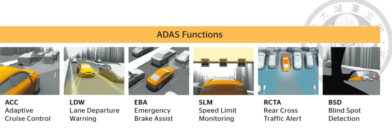
Since the most important thing is the safety of passenger and driver, advanced driver- assistance systems (ADAS) is developed to support enhanced vehicle system for safety and better driving. The purpose of ADAS is to enhance traffic safety and efficiency.

For example, ADAS are composed of autonomous emergency braking system (AEBS), adaptive cruise control (ACC), lane departure warning (LDW), speed limit monitoring (SLM), rear cross traffic alert (RCTA), blind spot detection system (BST).

These subsytems provide different effects for better driving. Lane departure warning warns the driver if ADAS detects that the vehicle is departing from the current lane.

Adaptive cruise control is used to handle the vehicle speed adaptively based on the distance between your vehicle and leading vehicle, your current speed, the road condition, and prediction of the leading vehicle’s speed change. Automatic emergency braking system is a system that automatically detect a potential forward collision and trigger the vehicle braking system to decelerate the vehicle with the purpose of avoiding or mitigating

(12)

ACC Adaptive Cruise Control

LDW

Lane Departure Warning

ADAS Functions

Sensors for Advanced Driver Assistance Systems (ADAS)

EBA Emergency Brake Assist

SLM Speed Limit Monitoring

RCTA Rear Cross Traffic Alert

BSD Blind Spot Detection SRL

Short Range Lidar

ARS Advanced Radar Sensor

MFC

Multi Function Camera SRR

Short Range Radar

Advanced Development

›Special sensor adaptations for R&D in field of autonomous driving

›Assistance in selection and specifica- tion of environmental sensor systems

›Feasibility and design studies

›Function concepts

›Development and implementation of algorithms

›Simulation and Evaluation

›Conception of Prototypes

Prototypes

›Prototype design

›Integration of sensors and components in ADAS demonstration vehicles and test equipment

›Sensor calibration

›Assistance during initial operation and pilot projects

›Gateways

›Software adaptations

›Rapid prototyping of new algorithms

›Testing

Series Applications

›Application of environment sensors (radar, infrared and camera systems)

›Project management

›Requirements management

›Release planning

›Test vehicle build up

›CAN / Flexray

›Function development

›Function calibration

›AUTOSAR

›Software integration

›Diagnosis

›Feasibility and design studies

›Function concepts

›Algorithm development

›Software adaptation

›Test measurements

›Data analysis

›Prototype build up

›Series development for non-automotive applications

As well as the use of these sensors in automobiles, there are also applications for the use of these components in other sectors like agriculture and construction equipment. Here, our sensor customers can benefit from sensors that were developed under the high standards in the automotive industry and are produced in large numbers. We can find solutions for many applications in which previously in- house development was not profitable because of low numbers.

Special Software Application for non-automotive industries

Continental Engineering Services GmbH Graf-Vollrath-Weg 6 · 60489 Frankfurt /Germany Phone + 49 69 678696- 0 · Fax + 49 69 678696- 070 www.conti-engineering.com

Figure 1.1: ADAS functions¹

a collision if the driver fails to react to an emergency situation.

Nowadays, computer vision, together with radar and Lidar, is at the forefront of technologies that enable the evolution of AEBS. Figure 1.2 shows an example of ADAS sensors. Radar offers some advantages, such as long detection range (up to 200 m) and capability to operate under extreme weather conditions. However, it acts awful on false positives, especially around road curves, because it is not able to recognize objects. Lidar, which is commonly spelled LiDAR and also known as LADAR or laser altimetry, is an acronym for light detection and ranging. It is a surveying method that measures distance to a target by illuminating that target with a pulsed laser light, and measuring the reflected pulses with a sensor. Although both radar and lidar are precise and have long range, lidar has more resolution than radar sensors. So lidar is popularly used to make high-resolution maps in these days [2] [3] [4]. For example, Google’s self-driving car [5] relies on lidar to provide it with a 360 degree of what is happening around the vehicle. It has a lidar sensor attached to the top of a car where it spins and shoots out lasers to create high-resolution maps of the car’s surroundings. Camera-based systems also have their own limitations.

They are very sensitivity to weather conditions, and they are not as reliable as radar when obtaining depth information. On the other hand, they have a wider field of view, and more importantly, they can recognize and categorize objects.

However, the cost of long range radar or lidar is very high. Lidar is the most expensive

1Source: http://www.conti-engineering.com/CMSPages/GetFile.aspx?guid=cf6d6925-8148-46e9- b59a-6eed8c23a0f6

2Source: Advanced Driver Assistant System - Intel, https://www.intel.com/content/dam/www/public/us/en/documents/white- papers/advanced-driver-assistant-system-paper.pdf

(13)

This system is considered as a close-loop control system, where the vehicle control actuation actions are computed based on received data from sensors. And the outcome of the ADAS actuation actions is fed back in the loop as sensor input. All the computing units in ADAS of the vehicular system are generally referred to as electronic control units (ECUs). The sensing and actuation ECUs are relatively resource constrained units, compared with the central processor of ADAS.

One of the key advancements in ADAS design is the concept of “sensor fusion.” This is the process by which the internal processing takes input from the multiplicity of external sensors and creates a map of possible impediments around the vehicle. The map then facilitates the computation that creates a series of possible actions and reactions through situational analysis. Figure 3 shows an example ADAS-enabled vehicle with a collection of sensors to enable sensor fusion and actions.

Figure 2. Conceptual Hardware Block Diagram for ADAS System

Figure 3. Example ADAS Sensors SMART

SENSOR SMART

ACTUATOR

SMART ACTUATOR SMART

SENSOR

SMART SENSOR

SENSOR

PROCESSOR CENTRAL

PROCESSOR RAM

ROM RAM ROM

CLOCK

ASILD WDT

POWER

SENSOR COMMUNICATION PROTOCOL COMMUNICATION PORTAL COMMUNICATION PORTAL

VIDEO

CAMERA REVERSE

CAMERA NIGHT VISION

CAMERA

ULTRASOUND MID RAN E

RADAR BACK MID RAN E

RADAR FRONT LON RAN E

RADAR

4

Advanced Driver Assistant System:

Threats, Requirements, and Security Solutions

Figure 1.2: An example of ADAS sensors.²

component in these sensors. A single unit of lidar cost 75,000 US dollars just a few years ago. Although Google’s self-driving car project-turned-spinoff company claim to slash the price of lidar by 90%, it stills cost 7,500 US dollars per vehicle [6]. Therefore, we want to study by using only camera-based system to construct AEBS system. There are many kinds of camera now, like short/long focal length, digital/optical zooming...etc.

Choosing a suitable camera plays an important role in our camera-based system. The wide-angle camera (wide field of view) eventually reaching the super wide-angle range, which capture an even broader scope. On the other hand, the object will be very small when it is far from the camera. The telephoto camera restricts the angle of view, but it is capable to capture faraway objects at a larger size. If we use only wide-angle camera to detect the objects, we may miss some vehicles which are far from us. On the other hand, we may miss vehicles in a traffic jam (only the part of vehicles in the FoV) if we choose telephoto camera.

For all these reasons, our proposed heterogeneous camera-based system on AEBS will use sensor fusion to combine the strengths of all the difference field of view (FoV) cameras. There are some purposes to fuse information from the heterogeneous camera sensors

(14)

Figure 1.3: An example of different FoV camera. (a) wide-angle camera. (b) focal length between wide-angle camera and telephoto camera. (c) telephoto camera.

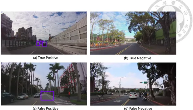
of ADAS. First, to make content of some information more complete. Second, to improve the accuracy of the sensor-detecting information. Final, to improve the robustness of the sensor-detecting information. Although the true positive (shown in Figure 1.4(a)) of the AEBS system will be increased by using sensor fusion to fuse all the different FoV cameras, however, the false positive will be increased as well. As all the ADAS systems are computer-based and depend on sensor technology, data fusion, and image analysis. False positive instances (false alarms) or error of the system are unavoidable. Since the false positives may cause a fatal malfunction of a vehicle, and it may result in dangerous accidents. It is important to reduce the occurrences of false positives to improve the robustness and reliability of the system. For example, Figure 1.4(c) shows a false positive detection.

In this case, the "car" rectangle is detected by vehicle detection algorithm. AEBS will automatically stop the car to avoid the accident because of this false positive detection.

However, this unnecessary emergency brake activation doesn’t make sense since there is no cars ahead. Further, this reaction may cause a rear-end accidents.

Because of the above mentioned, our work will develop a heterogeneous camera-based system on AEBS, which has not only the advantage of all the different FoV cameras, but also the lower false positive rate.

(15)

Figure 1.4: An example of true positive, true negative, false positive, false negative.

1.2 Contribution

In this thesis, we propose a heterogeneous camera-based system for AEBS. Compare to others camera-radar based system, the AEBS can be set up in a lower cost by using our system. Also, the proposed system guarantees higher accuracy and lower false positive rate than single monocular camera system. At last, we optimize the proposed sensor fusion method because of the the limitation of computing resource on embedded system.

1.3 Thesis Organization

The remainder of the thesis is organized as follows. In Chapter 2, we present previous existing fusion functions for heterogeneous sensors and related works. In Chapter 3, we present our system architecture. In Chapter 4, we present our algorithm and we use R-tree to reduce the search space. In Chapter 5, we evaluate our algorithm and present the results of our experiments. Chapter 6 conclude our work in this thesis.

(16)

Chapter 2 Background and Related Work

2.1 Autonomous Emergency Braking System

In recent years, Europe, America and other developed countries have spent enormous efforts in developing ADAS, AEBS as an important part of the ADAS has become a popu- lar research topic. To ensure safety, UNECE R131 [7] defines the functional requirements of AEBS. Here are the definition in UNECE R131. The subject vehicle refers to the tested vehicle which is the category M3 vehicle. The target refers to a high volume series pro- duction passenger car of category M1 AA saloon¹ or in the case of a soft target. Time to collision (TTC) refers to the interval of time obtained by dividing the distance between the subject vehicle and the target by the relative speed of the subject vehicle and the target, at an instant in time.

The subject vehicle shall approach the stationary target in a straight line. The functional part of the test shall start when the subject vehicle is traveling at a speed of 80

± 2 km/h and is at a distance of at least 120m from the stationary target. First, at least one warning shall be issued no later than 1.4s before the start of emergency braking phase.

Second, at least two warnings shall be provided no later than 0.8s before the start of emergency braking phase. Final, the emergency braking phase shall not start before the TTC is equal to or less than 3.0 seconds.

1As defined in the Consolidated Resolution on the Construction of Vehicles (R.E.3.), document ECE/- TRANS/WP.29/78/Rev.2, para. 2.

(17)

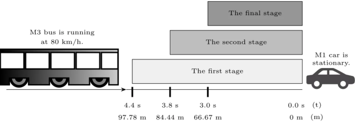
Since AEBS should have at least one warning no later than 1.4s before the start of emergency braking phase and the emergency braking phase shall not start before the TTC is equal to or less than 3.0 seconds by the regulation, AEBS should issue at least one warning when TTC is equal to or less than 4.4s. In the same way, AEBS should issue at least two warnings when TTC is equal to or less than 3.8s. As a result of above, we need to detect if the stationary target vehicle exists when TTC is equal to or less than 4.4s and TTC is equal to or less than 3.8s.

By the formula of constant velocity motion (s = v ⇤ t), we can obtain that the distance between subject vehicle and stationary target is 97.78 meters when the speed of subject vehicle is 80km/h and TTC is equal to or less than 4.4s.

4.4 s 97.78 m

3.8 s 84.44 m

3.0 s 66.67 m

0.0 s 0 m The first stage

The second stage The final stage

(t) (m) M3 bus is running

at 80 km/h.

M1 car is stationary.

Figure 2.1: AEBS-TTC testing. (a) The first stage: at least one warning mode shall be provided. (b) The second stage: at least two warning mode shall be provided. (c) The final stage: the emergency braking phase shall start.

2.2 Vision-Based Vehicle Detection - YOLO

A large amount of researches which are computer vision based have been conducted on vehicle detection from over the years. Many of them applied traditional methods, such as background subtraction, frame difference, optical flow, etc. In [8], they applied a median-based background subtraction method to detect vehicles. In [9], they proposed a frame difference method to detect moving vehicles. However, our research targets a

(18)

dynamic background, which is collected by a camera, meaning that traditional methods such as frame difference, background subtraction cannot be used directly.

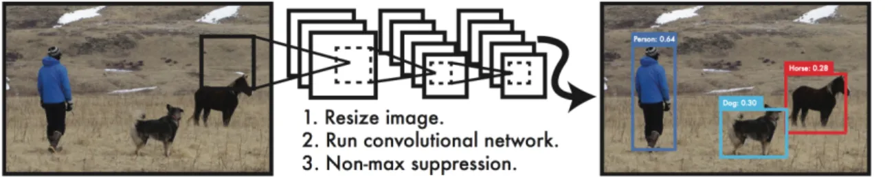
Since deep learning has become a powerful technology in image recognition, gaming, information retrieval, and many other areas that need intelligent data processing. There are several machine learning based approaches have been proposed on vehicle detection in last few years. You Only Look Once (YOLO) [10] [11], a machine learning based algorithm which is proposed by Joseph Redmon at 2016, is a new and effective method to detect objects based on regression instead of classifying. Different from others machine learning algorithm (like R-CNN), the image is only fed into the YOLO network just for once and the network can output all the detect results. The workflow of YOLO detection system is shown in Figure 2.2. First, the system resizes the input image to 416 × 416 pixels. Second, it runs a single convolutional network on the image. At last, it filters the resulting detections by the model’s confidence. Compared to traditional methods of object detection, processing images with YOLO is simple and straightforward. Also, YOLO is extremely fast and it is capable to detect a wide variety of object classes. It can detect over 9000 object categories and it runs at 67 frame per second (FPS) on a Geforce GTX Titan X [11].

Figure 2.2: The YOLO detection system²

2Source: J. Redmon and A. Farhadi., “Yolo9000: Better, faster, stronger.” in Computer Vision and Pattern Recognition, 2016.

(19)

2.3 R-tree

R-tree is a hierarchical data structure proposed by Antonin Guttman [12] in 1984. It is based on B-tree and can be used to search spatial objects efficiently. Similar to the B-tree, the R-tree is also a balanced search tree, within which all leaf nodes are at the same height. R-tree is a well known spatial indexing technique that has been widely used in many geospatial applications, like indexing 2D or higher dimensional data. A common real-world usage for R-tree is to store spatial objects such as restaurant locations, streets, buildings informations, and then find answers to query such as "Find all restaurant within 1 km of my current location".

The main idea of R-tree is to group nearby objects and represent them by their minimum bounding rectangle (MBR) in the next higher level of the tree. The R-tree data structure consists of intermediate nodes and leaf nodes, and each node consists of several entries. Data objects are stored in leaf nodes and intermediate nodes are built by grouping rectangles at the lower level. Each entry of intermediate node is associated with MBR within which some rectangle completely encloses all rectangles that correspond to lower level nodes. Intermediate nodes contain entries of the form (Rect, child-ptr) where child- ptr is a pointer to a child node in the R-tree; Rect is the MBR that covers all rectangles of the child node. Leaf nodes contain entries of the form (Rect, tuple-identifier) where tuple- identifier is a pointer to the object description, and Rect is the MBR of the object. The main innovation in the R-tree is that parent nodes are allowed to overlap. This way, the R-tree can guarantee at least 50% space utilization and remain balanced [13]. In R-tree, the MBR of root node covers all rectangles and the leaf nodes store the information of data objects. Let us assume that M is the maximum number of entries that can fit in a leaf or intermediate node, m is the minimum number of entries that must fit in an intermediate node. The R-tree has the following properties:

(i) The root node has at least two children unless it is a leaf.

(ii) The entries number of entries on intermediate node should be no less than m and no greater than M.

(20)

The first step of constructing R-tree is to generate MBR for the data rectangles. The next step is to group nearby rectangles and group them into a new MBR that is large enough to cover the rectangles in the next higher level of the tree. This process will continue until the root of R-tree is found, which is the rectangle covering all data rectangles.

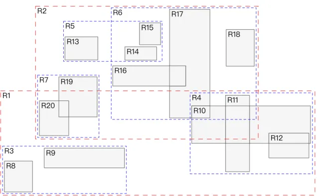
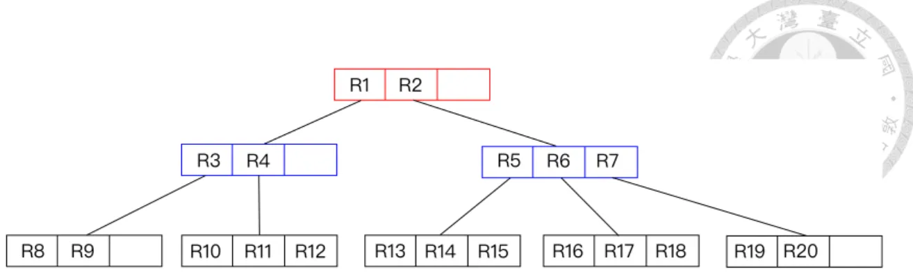
Figure 2.3 shows an example set of data rectangles. For example, at the first step, each data rectangle (gray rectangle) generates its MBR. At the next step, the data rectangles are divided into several groups, and the new MBRs (blue rectangles) are generated to cover each group of data rectangles. In this case, R5 is the MBR which is created in this step and it covers the data rectangle R11 and R12. The process will continue until the root of R-tree is found, which are red rectangles in this case. The final result of this construction is shown in Figure 2.4, which is the corresponding R-tree built on these data rectangles (assuming a maximum branching number M = 3 and minimum branching number m = 2).

Figure 2.3: Data (gray rectangles) organized in a R-tree with M = 3, m = 2

Since the main idea of R-tree is to group nearby objects and represent them with their minimum bounding rectangle (MBR) in the next higher level of the tree. The key idea

(21)

Figure 2.4: R-tree (with M = 3, m = 2) for the data rectangles of Figure 2.3

of searching algorithm in R-tree is to use the bounding boxes to decide whether or not to search inside a subtree. In this way, most of the nodes in the tree are never read during a search. Like B-tree, this makes R-tree suitable for large data sets and databases, where nodes can be paged to memory when needed, and the whole tree cannot be kept in main memory. Assuming M is the maximum number of entries that can fit in a leaf or intermediate node, N is the number of leaf nodes. The time complexity of searching algorithm is O(logMN ). Due to the searching algorithm, the performance of R-tree depends on the quality of the algorithm that clusters the data rectangles on a node. If the cluster algorithm results in several overlapping between MBRs, the performance will degrade because of the increasing of the searching subtrees.

In this thesis, we assume that the data rectangles are static (do not require dynamic insertions or updates). The low-x packed R-tree [14] is a step towards to construct an R-tree with 100% space utilization which will have as good response time as possible at the same time. However, this method will result in degradation of performance for region queries. Hilbert R-tree [15] is proposed by I. Kamel in order to cluster the region data in a better way than the low-x packed R-tree. Instead of sorting the data on the x or y coordinate, Hilbert R-trees use the Hilbert curve to impose a linear ordering on the data rectangles. The basic Hilbert curve on 1x1, 2x2, 4x4 grid are shown in Figure 2.5. The number in each grid presents Hilbert value. For example, on the 4x4 grid (denote by H2, the (0,0) is at lower left corner), the point (0,0) on the H2 curve has a Hilbert value of 0, while the point (2,1) has a Hilbert value of 13. Also, the Hilbert value of a rectangle needs to be defined. Following the experiments in [13], a good choice is that the Hilbert

(22)

value of a rectangle is defined as the Hilbert value of its center.

0

1 2

3 0 1

3 2 4

5 6

7 8

9 10

11

12 13

14 15

H H H

1 2 3

Figure 2.5: Hilbert curves of order 1, 2 and 3 [15]

The Hilbert R-tree claims that the overlapping between MBRs will decrease by using the ascending Hilbert value to pack the rectangles during the construction of R-tree. Since the performance of Hilbert R-tree is better and the construction cost is low (only change the packing rules from the original R-tree), we will use Hilbert R-tree in this thesis.

2.4 Related Work

Various approaches are taken to build ADAS platforms nowadays, with focus being reliability, high performance, low cost and low power consumption. These platforms usu- ally contain a few processing units with different purposes on the same system on chip (SoC). There are several research focus on heterogeneous sensing fusion. That is, they use camera and radar or other sensors together [16] [17] [18] [19]. In [16], they propose a vehicle recognize algorithm base on radar and vision sensors with the application to automatic emergency braking. Since the radar is sensitive, there are a lot of false detection caused by radar. To improve this, they propose a vehicle recognition method which is based on shape and motion attribute. The motion attribute is designed to determine whether the object is either stationary or dynamic and the shape attribute aims to identity

(23)

whether the objective is a vehicle or not by sensor fusion. In [17], they use mobile smart phone as a computing platform because the mobile smart phones today are equipped with numerous sensors that can help to aid in safety enhancements for drivers on the road.

In [18], they use informations that are provided by in-vehicle Lidar and monocular vision to present a detect, track and classify entities in semi-structured outdoor scenarios.

In [19], they use radar and camera to recognize whether the detected object is either vehicle or non-vehicle with the application of AEBS. Most of the researches use different type of sensors simultaneously on AEBS. Different from them, we use only camera-based system to construct AEBS system.

(24)

Chapter 3 System Architecture and Problem Definition

3.1 System Architecture

Safety-critical embedded systems are undergoing an evolution towards greater auton- omy. In this thesis, we use the recently released NVIDIA Jetson TX2 as our computing platform. Since we use a GPU-based deep learning (YOLO) as our vehicle detection algorithm and several different FoV cameras simultaneously, the computing platform we used must have GPU to run YOLO system and suppors for multiple cameras module. Also, this computing platform should be portable because the ADAS is running on moving vehicles.

Moreover, this computing platform should have low power consumption since the energy on vehicle is limited. Thus, NVIDIA Jetson TX2 is one of the most suitable computing platform for us due to these limitation.

NVIDIA Jetson is the world’s leading AI computing platform for GPU-accelerated parallel processing in mobile embedded systems and is called for "autonomous every- thing" [20]. NVIDIA Jetson TX2 is part of the Jetson family of embedded computers.

It shares a common GPU architecture with the higher-end NVIDIA Drive PX2, which is currently available only to automotive companies and suppliers. It is one of the most outstanding GPU-enabled platforms marketed today for autonomous systems. It has two

(25)

important attributes for embedded use cases. First, it provides significant computing ca- pacity. Second, it meets pratical limits on monetary cost as well as size, weight, and power consumption. It doubles the performance of its predecessor. And it can run at more than twice the power efficiency, while drawing less than 7.5 watts of power [21]. Figure 3.1 shows the capability of NVIDIA Jetson TX1 and TX2.

Figure 3.1: The ability of NVIDIA Jetson TX1 and TX2¹

We set up three different FoV cameras at the same view direction on this platform.

Figure 3.2 shows the proposed heterogeneous camera-based system on vehicle with a collection of sensors to enable sensor fusion and actions. For simplicity, we use normal camera to represent the camera which focal length between wide-angle camera and telephoto camera. In the rest of this thesis, the term "wide-angle camera", "normal camera"

and the term "telephoto camera" will be used frequently. The horizontal angle of wide- angle camera is 150 , which covers all two lanes next to the vehicle. The horizontal angle of normal camera is 52 , which covers part of two lanes next to the vehicle and the lane that the moving vehicle is traveling at. The horizontal angle of telephoto camera is 28 , which only cover the lane that the moving vehicle is traveling at.

(26)

wide-angle camera 150^o

normal camera 52^o telephoto camera 28^o

Figure 3.2: The architecture of the proposed heterogeneous camera-based system

In this thesis, we assume that the real-time clocks of all the cameras are synthesized, and all the camera frames are merged into a single frame in advance. Figure 4.2 shows the single frame composed by three different FoV camera. The frame at lower left corner comes from wide-angle camera, the frame at upper half comes from normal camera, and the frame at lower right corner comes from telephoto camera. The red rectangls are the region of interest (ROI) since AEBS only concern the target vehicles in front of the subject vehicle.

3.2 Problem Definition

The target problem is to increase the recall of vehicle detection algorithm (YOLO system) by using sensor fusion for heterogeneous camera-based system and optimize the sensor fusion method since the computing resource on embedded system is limited. Ac- cording to the regulation of UNECE R131 [7], AEBS should start the emergency braking phase before a TTC equal to or less than 3.0 seconds. As shown in Figure 2.1, when the

(27)

distance between the target vehicle and the subject vehicle equal to or less than 66.67m, the final stage should start the emergency braking phase. Thus, the proposed heterogeneous camera-based system should have the ability to detect the target vehicle when the distance between the target vehicle and the subject vehicle equal to or less than 66.67m.

Another problem is to decrease the false positive rate since there are some false detections that caused by the sensor fusion method.

(28)

Chapter 4 Design and Implementation

In this chapter, we design the heterogeneous camera-based system and implement sensor fusion method and false positive removal method on it. Figure 4.1 shows the data flow of the heterogeneous camera-based system. First, we discuss the impact of input image size on YOLO system in Section 4.1. Second, we need to transform all the detected vehicle rectangles from different FoV cameras into the same coordinate system before we design the sensor fusion method to fuse all the detected vehicle rectangles from different FoV cameras. We use linear transformation to transform the coordinate system in Section 4.2. After that, we use existed sensor fusion method into the system in Section 4.3. However, the effect of existed sensor fusion method in the night scenario is not significant enough. Thus, we proposed an advanced sensor fusion method in Section 4.4. Unfortunately, we may increase the false positive rate during the sensor fusion. The higher false positive rate may cause the system do more illogical operations during car driving. Thus, we proposed a false positive removal method to decrease the false positive rate in Section 4.5. Finally, since the computing resource on embedded system is limited, we need to reduce the search space of the proposed sensor fusion method. The discussion of reducing search space is in Section 4.6.

(29)

Wide-angle camera video (1920x1080 pixels)

Normal camera video (1920x1080 pixels)

Telephotoc amera video (1920x1080 pixels)

Wide-angle camera video (416x416 pixels)

Telephoto camera video (416x416 pixels) Normal camera video

(416x416 pixels)

Coordinate System Transformation Crop

Search Space Reducation

Sensor Fusion

False Positive Removal

Result

Figure 4.1: Data flow of the heterogeneous camera-based system.

(30)

4.1 The Impact of Input Image Sizes

As we mentioned at section 2.2 , YOLO will resize the input image to 416 x 416 pixels before it feeds the input image into the convolution network. If the system uses a single frame which frame size is 1920 x 1080 pixels as an input image, YOLO will resize it into 416 x 416 pixels in advance. Consequently, the recall of using frame that frame size is 1920 x 1080 pixels as input image is worse than using frame that frame size is 416 x 416 pixels as input image. Table 4.1 shows the result of it. To solve this problem, the system crops the frame into several images which size are 416 x 416 pixels before the system invokes the YOLO system. As shown in Figure 4.2, the system crops a 416 x 416 pixels image (denote to the red rectangles) from each camera. These red rectangles are the region of interest (ROI) of wide-angle camera, normal camera, and telephoto camera since AEBS only concerns the target vehicles in front of the subject vehicle.

Size of input image (pixel) Recall

1920 x 1080 45%

416 x 416 94.5%

Table 4.1: Recall of object detection using YOLO

Figure 4.2: The frame that composed by three different FoV camera and the ROI of each camera.

(31)

4.2 Coordinate System Transformation

In order to fuse all the vehicle rectangles that detected by different FoV cameras, we demand to transform these rectangles into the same coordinate system, which is "global coordinate system". In this chapter, we use N1 to represent for wide-angle camera, N2

to represent for normal camera, and N3 to represent for telephoto camera. We use the linear function to transform the position of the detection rectangles into global coordinate system, and it can be shown as follows:

xi0 = xi

magi

+ X_i^o↵set yi0 = yi

magi

+ Y_i^o↵set

(4.1)

where xi and yirepresent the position in the coordinate system of camera Ni; xi0 and yi0

represent the position in the global coordinate system; magirepresents the magnification of camera Ni ( That is, mag1 = 1, mag2 = 2, and mag3 = 4 ); X_i^o↵set represents the translation offset of xi0 in global coordinate system, and Y_i^o↵set represents the translation offset of yi0 in global coordinate system where

X_i^o↵set = W ⇤ (1 1 magi

) Y_i^o↵set = H⇤ (1 1

magi

)

(4.2)

W represents the width of croped input image of YOLO, and H represents the height of croped input image of YOLO.

4.3 Existed Sensor Fusion Method

As we mentioned at Section 2.2, YOLO filters the resulting detections by the model’s confidence after it runs a single convolutional network. In YOLO, the confidence threshold of vehicle is 0.2. Therefore, if the confidence of the detection is lower than 0.2, this detection will be filtered out by YOLO. However, there are some detections that are true positive but its confidence is lower than the threshold. These detections will be filtered out

(32)

by YOLO although they are true positive. If we integrate the low confidence detections from different FoV cameras, we can keep the true positives that are filtered out by YOLO system. Thus, we use an existed sensor fusion method, De Morgan’s law, to fuse the low confidence detections from different FoV cameras into a new detection. Once the confidence of the new detection is higher than the threshold, YOLO will not filter out this true positive detection. And the recall will be increased because of the increasing number of the true positive detections. The De Morgan’s law for three sensors A, B, C can be written formally as

A[ B [ C = A \ B \ C (4.3)

and the probability of the event detected by three sensors is defined as

P (A[ B [ C) = 1 (1 A)⇤ (1 B)⇤ (1 C) (4.4)

where P (A [ B [ C) denotes to the probability of A [ B [ C.

First of all, we use the method at Section 4.2 to transform all the vehicle rectangles that detected by different FoV cameras into global coordinate system. Second, we test if the detections from different FoV cameras denote to the same vehicle or not. Assume that the detection R1 is detected by camera N1, the detection R2 is detected by camera N2, and the detection R3 is detected by camera N3. In order to determine that the detections denote to the same vehicle, the overlap testing is defined as follows:

Overlap(R1, R2, R3) = 8>

><

>>

:

true ,area of intersection

area of union >Overlap threshold f alse , otherwise

(4.5)

and the value of Overlap threshold is 0.5 in this thesis. Once the detection R1, R2, R3from differents FoV cameras pass the overlap testing, we ensure that the detections R1, R2, R3

denote to the same vehicle. At last, we use De Morgan’s law to fuse these detections R1, R2, R3 into a new detection, which is R4. The position of R4 is determined by the intersection rectangle of R1, R2, R3, and we can obtain the confidence of R4by using De Morgan’s law:

(33)

C4 = P (C1 [ C2[ C3) = 1 (1 C1)⇤ (1 C2)⇤ (1 C3) (4.6) where C1 represents the confidence of R1, C2 represents the confidence of R2, C3 represents the confidence of R3, and C4 represents the confidence of R4.

4.4 Proposed Sensor Fusion Method

In this section, we propose a sensor fusion method that is based on De Morgan’s law, which is "Weighted De Morgan’s law". The significant difference between Weighted De Morgan’s law and De Morgan’s law is that we add a weighted function on it. The recallof different FoV cameras are different when the distance between the target vehicle and the subject vehicle is the same. For instance, as shown in Figure 4.3, the recall of telephoto camera is higher than wide-angle camera when the distance between the target vehicle and the subject vehicle is 60 meters at night. At this distance, the confidence of detected vehicle rectangles from telephoto camera are more reliable than the rectangles that detected by wide-angle camera. On the other hand, the recall of wide-angle camera is higher than telephoto camera when the distance between the target vehicle and the subject vehicle is 10 meters at night. Because the capability of different FoV cameras under different distances are variaty, the weighted function in our proposed sensor fusion method will concern the capability of each camera.

The distance between the subject vehicle and the target vehicle is a significant information in the Weighted De Morgan’s law. Since our AEBS architecture is camera-based system, we apply a camera-based method to observe the distance between the subject vehicle and the target vehicle rather than using radar or lidar sensors to measure the distance. The distance measurement method is to utilize the length of vehicle width in camera to measure the distance. The length of the target vehicle width in camera depends on the distance between the target vehicle and the subject vehicle. For instance, Figure 4.4 shows that the target vehicle is place at different distances between the subject vehicle. In this thesis, we assume the minimum vehicle width is 1.5 meters. Figure 4.5

(34)

0 10 20 30 40 50 60 70 0

10 20 30 40 50 60 70 80 90 100

Distance (meter)

Recall(%)

Wide-angle Camera Normal Camera Telephoto Camera

Figure 4.3: The recall of different FoV camera when the target vehicle is placed at different distance at night.

Figure 4.4: The target vehicle is placed at different distances. (a) The distance is 10 meters. (b) The distance is 40 meters.

(35)

0 10 20 30 40 50 60 70 80 90 100 0

50 100 150 200 250

Distance (meter)

Vehiclewidth(pixel)

Figure 4.5: The length of the target vehicle width at different distances. The input frame size is 1920x1080 pixels and we assume the target vehicle width is 1.5 meters.

shows the experiment of the length of the target vehicle width at different distances between the subject vehicle. The weight in the Weighted De Morgan’s law is a function to the recall of each camera under the certain distance. For instance, when the distance between the target vehicle and the subject vehicle is 60 meters, the recall of wide-angle camera is 4.5, the recall of normal camera is 42.3 and the recall of telephoto camera is 83.3. Thus, the weight of wide-angle camera is 4.5/(4.5 + 42.3 + 83.3) ⇤ 3, the weight of normal camera is 42.3/(4.5 + 42.3 + 83.3) ⇤ 3 and the weight of telephoto camera is 83.3/(4.5 + 42.3 + 83.3)⇤ 3.

The Weighted De Morgan’s law for three sensors A, B, C can be written formally as

↵A[ B [ C = ↵A \ B \ C (4.7)

and the probability of the event detected by three sensors is defined as

P (↵A[ B [ C) = 1 (1 A)^↵⇤ (1 B) ⇤ (1 C) (4.8)

(36)

where P (↵A [ B [ C) denotes to the probability of ↵A [ B [ C. ↵, , and represents the weight of each camera.

The fusion step is the same as De Morgan’s law. Once the detections R1, R2, R3from different FoV cameras pass the overlap testing, we use Weighted De Morgan’s law to fuse these detections R1, R2, R3 into a new detection, which is R40. The position of R40 is determined by the intersection rectangle of R1, R2, R3, and we can obtain the confidence of R40 by using Weighted De Morgan’s law:

C₄⁰ = P (↵C₁[ C2[ C3) = 1 (1 C₁)^↵⇤ (1 C₂) ⇤ (1 C₃) (4.9)

where C40 represents the confidence of R40, ↵ represents the weight of the confidence C1 , represents the weight of the confidence C2, and represents the weight of the confidence C3. The value of ↵, , are defined as follows:

↵ = rD,N1

PT

k=1rD,Nk

⇤ T

= rD,N2

PT

k=1rD,Nk

⇤ T

= rD,N3

PT

k=1rD,N_k

⇤ T

(4.10)

where D represents the distance between the target vehicle and the subject vehicle, T represents the total number of cameras, rD,Nk represents the recall of camera Nk when the distance between the target vehicle and the subject vehicle is D.

4.5 False Positive Removal

Since the target vehicle will not change its position significantly between consequently frames, we can use the information from previous frames to remove the false positive noise. We use a heuristic algorithm to solve the problem of increasing false positive rate.

The main idea of this algorithm is using the information from previous frames to remove

(37)

the false positive in current frame. Here we use a buffer to store the information from previous frames. Once the detection R appears (no matter this detection R is produced by YOLO or Weighted De Morgan’s law) in current frame, we will check the buffer. If there are no others detections that confidence greater than 0.2 in previous frames appear at the same position, the detection R is considered as a noise and we will filter out the detection Ras a noise in current frame. Otherwise, the detection R will be kept in current frame.

At last, we add all the detections into our buffer. If the a new detection R⁰ appears at the same position as R in the next frame, the new detection R⁰ will be considered as a true positive since the detection R appeared at the same position before. Also, the buffer will update the information of the new frame and discard the information that past for a long time. The number of the stored frames depends on the buffer size.

Algorithm 1 False Positive Removal

1: R.lx/R.ly : the left up corner x/y of detection R.

2: R.rx/R.ry : the right down corner x/y of detection R.

3: R.confidence : the confidence of detection R.

4: Buff [x][y][Buff_SIZE] : the array buffer to store the information of previous frames.

5: for each detection R in current frame do

6: int pixels = 0;

7: for y = R.ly; y < R.ry; y++ do

8: for x = R.lx; x < R.rx; x++ do

9: int buff_count = 0;

10: for j = 0; j < Buff_SIZE; j++ do

11: if Buff[y][x][j] == true then

12: buff_count++;

13: end if

14: if buff_count > FrequencyThreshold then

15: pixels++;

16: end if

17: if R.confidence > 0.2 then

18: Buff[y][x][frame_id%Buff_SIZE] = true;

19: end if

20: end for

21: end for

22: end for

23: float IntersectArea = pixels / [(R.rx-R.lx) * (R.ry-R.ly)];

24: if IntersectArea < AreaThreshold then

25: ignore the detection R

26: end if

27: end for

(38)

4.6 Search Space Reducation

Before we use Weighted De Morgan’s law to enhance the confidence of the detections from different FoV cameras, we need to find out that which detections are denoted to the same vehicles in all detections. This problem can be transform to maximal clique problem. We can transform the detections in global coordinate system into a simple undirected graph. In the undirected graph, each node represents an entity (such as detection rectangle) and each edge represents that these two nodes pass the overlap testing. Notice that if the two nodes (denoted to the detection rectangles) are detected by the same camera, they will not be connected by an edge even though they pass the overlap testing. Figure 4.6 (a) shows an example of global coordinate system that the red rectangles represent the detections of camera N1, the blue rectangles represent the detections of camera N2, and the black rectangles represent the detections of camera N3. In this example, only (R1, R3), (R1, R5), (R3, R5), (R1, R3, R5), (R2, R4)pass the overlap testing. That is, we will fuse (R1, R3, R5)and (R2, R4)by using Weighted De Morgan’s law. As shown in Figure 4.6 (b), we transform the detection rectangles in global coordinate system into an undirected graph. In undirected graph, (R1, R3, R5)and (R2, R4)are the maximal clique. The result of maximal clique in the graph is the same as the overlap testing of all detection rectangles in global coordinate system. Thus, we proof that the problem of finding detections that are denoted to the same vehicles in all detections can be transform to maximal clique problem.

However, the maximal clique problem is NP-complete, and it can not be solved in the polynomial time. Since we want to construct a safety critical embedded real-time systems, the shorter response time of the system is better. Thus, instead of constructing all the detection rectangles in a large undirected graph, we construct several small undirected graph to reduce the cost of time. In each iteration, we will focus on a detection rectangles and construct an undirected graph for it. We only do the Weighted De Morgan’s law for the maximal clique who covers the node that we focus on in this iteration. Assume that we focus on R1 in this iteration. R1 only intersect to R2 ⇠ R6 in global coordinate system as shown in Figure 4.7. If we use all the detection rectangles to construct the

(39)

Time complexity

R₁

R₅

R₄

R₆

R₃

R₂ R₄

R₆

R₅

R₂

R₃ R₁

(a)

(a) (b)

Figure 4.6: An example of transforming the detection rectangles in global coordinate system into an undirected graph.

R₄

R₆

R₅

R₂

R₃ R₁

R₇ R₈

R₉

R₁₀ R₁₁

R₁₂

R₁₃

R₁₄

Figure 4.7: An example of global coordinate system.

(40)

undirected graph, there will be lots of nodes that don’t have the connection between R1

and itself. These nodes is invaluable when we are focus on R1. Thus, if we can use a search algorithm to find out the detections that pass the overlap testing with R1before we transform the detections from global coordinate system into an undirected graph, we can reduce the number of invaluable nodes in the graph.

We can use the regional of the vehicle detections to reduce the search space although we cannot solve the NP-complete problem in the polynomial time. Since the detected vehicle rectangles denote to represent the position of the target vehicles, these detected vehicle rectangles will appear closely in the global coordinate system. As shown in Fig- ure 4.8, the red rectangles are detected by wide-angle camera, the yellow rectangles are detected by normal camera, and the green rectangle is detected by telephoto camera. We can observe that the overlap between vehicles is seldom. The reason of the situaction is that light is straightforward in nature. Assume that there is another vehicle T⁰ in the front of the target vehicle T in Figure 4.8. The YOLO system cannot detect T⁰ because of the property of light. There will not have a detection that covers another detection under the camera-based system. Thus, the overlap situation between all the detections is limited.

That is why we can use a search algorithm to filter out those who cannot pass the overlap testing detections to reduce the search space to speed up the sensor fusion method.

Figure 4.8: An example of overlap situation.

(41)

R-tree is a known solution for solving the multi-dimensional information searching problem. It use hierarchical MBRs to obtain the better performance. For each frame, we construct a R-tree to store the detections in the global coordinate system. We can obtain the detection rectangles that the focused detection R intersect to by going through the R- tree once. Figure 4.9 shows an example of using R-tree to speed up the searching problem.

Figure 4.9 (a) is the result of transforming all the detections from each FoV camera into global coordinate system. The purple rectangles represent the detected vehicle rectangles.

Figure 4.9 (b) and (c) shows the progress of constructing R-tree for the detected vehicle rectangles. We assume a maximum branching number M = 3 and minimum branching number m = 2. The blue and green rectangles represent the MBRs of R-tree. Figure 4.9 (d) shows the constructed R-tree of this frame. Figure 4.9 (e) ⇠ (g) shows the progress of finding the detections that intersect to the focused detection by using R-tree (assuming we focus on the detection R4). We can observe that the nubmer of detections in the global coordinater system in Figure 4.9 (g) is less than Figure 4.9 (a).

The Grid method is also a known solution for searching algorithm. The Grid method divide the global coordinate system into several grids G. If a detection intersects to a grid Gi, then the detection will be added to the list of grid Gi. Different from R-tree, the detection in Grid method may appear twice, or even three times, four times in the lists of Gi. The usage of grids G in Grid method is similar to the MBRs in R-tree. We can obtain the detection rectangles that the focused detection R intersect to by using these grids G. First, we will check whether the focused detection intersect to grid Gi

or not. We only need to check the detections in the list of Gi if the grid Gi intersect to the focused detection. Figure 4.10 shows an example of using Grid method to speed up the searching problem. Figure 4.10 (a) is the result of transforming all the detections from each FoV camera into global coordinate system. The purple rectangles represent the detected vehicle rectangles. Figure 4.10 (b) shows that the global coordinate system is divided into several grids (we assume the global coordinate system is divided into 9 grids in this example). Each detection will be added into the grid list Gi if the detection intersect to the grid Gi. Figure 4.10 (c) shows all the content in grid lists from G1 ⇠ G⁹.

(42)

Figure 4.10 (d) and (e) shows the progress of finding the detections that intersect to the focused detection by using Grid method(assuming we focus on the detection R4).

Figure 4.9: An example of using R-tree to speed up the searching problem.

(43)

Figure 4.10: An example of using Grid method to speed up the searching problem.

(44)

Chapter 5 Performance Evaluation

In this chapter, we evaluate the experiment result of our design, including the recall of the sensor fusion method, the precision of false positive removal method and the performance measurement on NVIDIA TX2. Since the AEBS only concerns the target vehicle, the recall and precision below represents the recall and the precision of the target vehicle. Table 5.1 shows the definition of recall and precision. For the notation T Piand F Pi, we use intersection over union (IOU) to determine whether two rectangles is the same. If the IOU of the detected rectangle and the ground truth rectangle is higher than 0.5, we will count the detected rectangle into T Pi. Otherwise, we will count it into F Pi.

Notation Definition

G_i Ground truth rectangles of the target vehicles of frame i Di Detected rectangles of frame i

T P_i G_i\ Di

F Pi Di Gi\ Dⁱ F N_i G_i G_i\ Di

recall ^P_{size(T P}^P^{size(T P}ⁱ⁾

i)+P

size(F Ni)

precision ^P_{size(T P}^P^{size(T P}ⁱ⁾

i)+P

size(F Pi)

Table 5.1: Notation table

(45)

5.1 Evaluation of Sensor Fusion Method

In this section, we evaluate the recall of the sensor fusion method under different scenarios. Figure 5.1 shows the recall of different FoV cameras, De Morgan’s law and Weighted De Morgan’s law in the night scenario and Figure 5.2 shows the recall of different FoV cameras, De Morgan’s law and Weighted De Morgan’s law in the sunny scenario.

We can observe that the De Morgan’s law and Weighted De Morgan’s law have a significant effect on recall in the night scenario. In the sunny scenario, we can observe that the recall of telephoto camera is higher than 90% until the distance between the target vehicle and the subject vehicle is greater than 140 meters. Thus, the effect of De Mor- gan’s law and Weighted De Morgan’s law in the sunny scenario is smaller than the night scenario. Luminous intensity is the reason of this phenomenon. A camera’s shutter deter- mines when the camera sensor will be open or closed to incoming light from the camera lens. The shutter speed specifically refers to how long this light is permitted to enter the camera. "Shutter speed" and "exposure time" refers to the same concept, where a faster shutter speed means a shorter exposure time. In general, the cameras need more exposure time in the night scenario since the luminous intensity in the night scenario is lower than the sunny scenario. Besides, the focal length of telephoto camera is higher than other cameras. Therefore, the motion of a camera has a great effect on it during exposure. If the camera moves quickly during exposure, the result image will turn into a blurred image. Thus, the recall of telephoto camera in the night scenario is lower than the recall in the sunny scenario. Because the motion of a camera has a little effect on wide-angle camera and normal camera, the image will not be blurred so much as telephoto camera.

The non-blurred image from wide-angle camera and normal camera reinforcement the blurred image from telephoto camera during the sensor fusion method. This is the reason that why De Morgan’s law and Weighted De Morgan’s law have a signigicant effect in the night scenario. In summary, the difference of exposure time between night and sunny scenario results in the different effect on the recall of De Morgan’s law and Weighted De Morgan’s law.

(46)

0 10 20 30 40 50 60 70 0

10 20 30 40 50 60 70 80 90 100

Distance (meter)

Recall(%)

Wide-angle Camera Normal Camera Telephoto Camera Normal De Morgan’s law Weighted De Morgan’s law

Figure 5.1: The recall of different FoV cameras, De Morgan’s law, Weighted De Morgan’s law when the target vehicle is placed at different distance at night.

0 10 20 30 40 50 60 70 80 90 100 110 120 130 140 150 160 0

10 20 30 40 50 60 70 80 90 100

Distance (meter)

Recall(%)

Wide-angle Camera Normal Camera Telephoto Camera Normal De Morgan’s law Weighted De Morgan’s law

Figure 5.2: The recall of different FoV cameras, De Morgan’s law, Weighted De Morgan’s law when the target vehicle is placed at different distance at sunny.