A New Weighting Scheme with Multiple Classifiers Fusion for Image Classification

(1)

Volume 12, No.4, December 2007, pp. 509-526

A New Weighting Scheme with Multiple Classifiers Fusion for Image Classification

Y. C. Tzeng¹ K. S. Chen²

ABSTRACT

One of the key prospects of data fusion is focused on exploiting the complementary information among different sensors. In this paper, the multiple classifiers approach is utilized for the multisource classification/data fusion to fully utilize as much of the available information among different data sources as possible. Three different weighting policies (variance reduction technique, rms distance weighting, and average distance weighting) applied to the multiple classifiers approach are introduced.

The performance of each combination method was demonstrated and compared with the fusion of the SAR and optical images for the terrain cover classification. Experimental results show that the classification accuracy is dramatically improved by making use of the proposed method. In addition, both the multiple classifiers using the rms (root mean squared) distance weighting and the average distance weighting outperform that of using the variance reduction technique.

Key Words: Image fusion, SAR, terrain classification, Multiple Classifiers

1. Introduction

For remote sensing image classification, there exist several methods of data fusion 1-10 to approach different problems; each of them bears both some advantages and disvantages. By means of fusion, different sources of information are combined to improve the performances of a system. It aims at obtaining information of greater quality; the exact definition of ‘greater quality’ depends upon the application. The fusion procedures are categorized1 by their input/output characteristics in five categories:

Data in Data out, Data in Feature out, Feature in Feature out, Feature in Decision out, Decision in Decision out. It is seen that data fusion are held at different levels and is divided into three levels:

raw data level fusion, feature level fusion, and decision level fusion. One example of the applications of data fusion is the use of remote sensing images from various sensors to improve land cover classification accuracies. Remote sensing images may originate from single/multiple sensors at different spectral channels, different spatial resolutions or different time intervals. This corresponds to spectral, spatial fusion or temporal fusion. The merging of high spatial resolution data, panchromatic data, high spectral resolution data, and multispectral data, allows us to obtain high spatial and spectral resolution at the same time.

The synergetic usage of different sensors allows us to review valuable information from the abundances of the extended spectral channels and the higher qualities of improved spatial

1 Professor, Department of Electronics Engineering, National United University

2 Professor, Center for Space and Remote Sensing Research, National Central University

Received Date: May 28, 2007 Revised Date: Dec. 26, 2007 Accepted Date: Dec. 27, 2007

(2)

resolution as well. Different sensor technologies have distinct or even complementary features. In principle, different targets (geometrical and physical properties) may respond differently to specific spectral frequencies within a bandwidth.

For example, optical imagery and SAR data show different advantages when used for land cover classifications and object detection in earth remote sensing. Hence, the important prospect of data fusion is focused on exploiting the complementary and yet supplementary information among different sensors. Proper data fusion can take advantage of the use of complementary information to obtain a better overall accuracy than using single source data only. Improper data fusion only makes thing worse.

Conventional parametric statistical classification methods are not appropriate in classification of multisource data, since in most cases they cannot be modeled by a convenient multivariate statistical model 11-12. A possible solution is to adopt a nonparametric approach, which does not rely on a specific distributional assumption and allows the kind of distribution to be derived entirely from data. Benediktsson et al.13 utilized a consensus theory to combine single probability distributions to summarize estimates from multiple experts (data sources) with the assumption that the experts make decisions based on Bayesian decision theory. A method of statistical multisource analysis was argumented to include mechanisms to weigh the influence of the data sources in the classification.

Datcu et al.7 adopted the concept of dependence trees for the integration of multisource information through estimation of probability distributions to apply a statistical approach to the

classification of multisource remote sensing data.

An Nth order binary distribution was approximated by a product of (N-1) second- order class conditional distributions. Then, a nonparametric method based on Gaussian kernels was used to estimate the second-order class conditional distributions.

Another attractive nonparametric approach is neural networks approach. It have shown promise in data fusion of multisource data and its powerful capability to model class posterior probabilities makes it an interesting solution to the classification problem. The other advantage of neural network methods is that no prior statistical information is needed about the input data. Still another interesting nonparametric approach is multiple classifiers. Its aim is to determine an effective combination method that makes use of the benefits of each classifier but avoids the weaknesses. The final decision (classification) was made based on the majority vote from all the classifiers. Tumer and Ghosh14 have shown that substantial improvements on classification performance can be achieved by combination or integrating the outputs of multiple classifiers. Wolpert15 introduced the stacked generalization scheme for minimizing the classification error rate for one or more classifiers. The outputs from classifiers are combined in a weighted sum with weights that are based on the individual performance of the classifiers. Benediktsson et al.12 applied a parallel consensual neural network in classification/data fusion of multisource remote sensing and geographic data. The input data were transformed several times and the different transformed data were used as if they were independent inputs. Then, the independent

(3)

inputs were classified, weighted and combined to make a consensual decision. Extended references on multiple classifier system may be found in 16.

In the next section, three different weighting policies that are applied to the multiple classifiers approach are introduced. In Section 3, the performances of utilizing the multiple classifiers approach to the application of multisource classification are compared.

Finally, some conclusions are drawn in Section IV.

2. Image Classification and Fusion

In image classification, the position vector of a class or cluster center ω_c is assumed to be the feature vector average of all the patterns in class (or cluster) c; that is, to adjust the position vector of the cluster center ω_c by minimizing the cost function17-21

∑∑

= =

= ^N^t

i M c

c

d i

J

1 1

2( , )

)

(Ω z ω (1)

M is the number of classes, )

, , , ( ₁ ₂

Nt

z z z

Z= L is a set of N_t training vectors; Ω=(ω₁,ω₂,L,ω_M) is the cluster center of Z; d(z_i,ω_c) is the distance measure between the ith training pattern and the cluster

c_.

In the search for the minima of the cost function in (1), it is highly efficient to apply a neural network algorithm. The major disadvantage of the neural network however, is that for most users it represents a black box.

Nevertheless, extensive research4, 11-12, 18-22 has shown that it is a powerful tool for handling

complex problems involving bulky volume set data in high dimensional feature space. A neural network, combined with fuzzy logic, has also been devised for remote sensing image classification. In DLNN(dynamic learning neural network)18-21, the input-output relationship of the network can be generally expressed as

x W

yr = r (2) where the output vector yr contains all the output nodes, xr is a long vector containing all the input and hidden nodes in a network, and matrix W is formed by concatenating all the weights connected to the output nodes. This modified perceptron structure allows the use of the Kalman filtering algorithm to update the weights during the learning process. This is important, because the implementation of the standard Kalman filter ensures the fast computation of the necessary parameters during the course of learning, namely, the weight updating. Weight updating affects the speed of network learning, which is a key concern when applying the neural network. Weight updating is based on the following criterion

DL M

c N i

i N c ci

t − <ε

∑∑

= =

+

1 1

1x w y

, (3) where N_t is the total number of input training patterns, and y_ci is the desired output of class c specified by the supervising users. The error bound,

ε

_DL , can be determined by the users, say, 1%. In a crisp network, we havey_ci∈{0,1}. The detailed implementation of DLNN can be found in18-21.

A data fusion can be modeled as an M hypothesis detection problem with hypothesis

Θ

m∈

θ

, where N individual detector decisions

(4)

zn form the observations Z

} ...

, {

z= z₀ z₁ z_N₋₁ ∈ 23-24. The observation space Z is split into disjoint regions, so that given an observation x, then hypothesis

θ

_i is chosen if z∈Z_i . The risk function for this decision is then

)

| z ( ) ( _ij _jj _j

Z j

jj

j P p

P

i j j

θ λ

− λ +

λ

=

ℜ

∑ ∑∫ ∑

θ

− Θ

∈ θ Θ

∈

θ (4)

where

λ

_ik is the cost associated with choosing hypothesis

θ

_i when

θ

_j is true,

) ( _j

j p

P =

θ

is the a priori probability of hypothesis

θ

_j, and p(x|

θ

_j)is the conditional probability of x given that

θ

_jactually occurred, so

∫

X p(x|θj) is the probability of choosing

θ

iwhen

θ

_jis true.

In (4), the first term is the fixed cost and the second term is the cost dependent on the choice of decision boundaries. To minimize the risk function , we need to know th e a priori probability of hypothesis

θ

_jand p(x|

θ

_j). But they are hard to know. For fusion of SAR and o p t i c a l i m a g e s , w e m a y a s s u m e t h a t

)

| ( )

| x (

1

0

θ θ

∏

⁻

=

= ^N

i

xi

p

p b y t h e a r g u m e n t o f independency of the sensor systems. To implement the minimization of the risk function in (4), we seek to combination strategies as will be illustrated in the following.

3. Combination of Multiple Classifiers

The final decision is made by fusing information from individual data sources after each data source has undergone a preliminary classification. To fusing the preliminary classification information, a weighting policy is

applied to the intermediate (unencoded) output of each classifier rather than the encoded output.

In this paper, we examined three methods to combine the outputs from each classifier.

As shown in Fig. 1, let X be an output random variable of a classifier, and we want to estimate

μ

=E( X). Suppose that Y is a random variable of another classifier involved in the classification that is assumed to be correlated with X, and that we know the value of

ν

=E(Y). Let c be a constant that has the same sign as the correlation between Y and X. We use c to scale the deviation Y −ν to arrive at an adjustment to X and thus define the controlled estimator

(

−

ν )

−

= X cY

X_c (5) Note that if Y and X are positively correlated, so that c > 0, we would adjust X downward whenever Y >ν and upward whenY <ν ; the opposite is true when Y and X are negatively correlated, in which case c < 0. In this way, we use the knowledge of Y’s expectation to pull X (down or up) toward its expectation

μ

, thus reducing its variability about

μ

. Since E( X)=

μ

and E(Y)=

ν

, it is clear that for any real number c, E(Xc) =

μ

; that is Xc is an unbiased estimator of

μ

that might lower variance than X. Specifically,

( )

X Var( )X c Var( )Y cCov(X,Y)

Var c = + ² −2 (6)

so that Xc is less variable than X if and only if

(

X Y

)

c Var

( )

Y cCov , ²

2 > (7) To find the best value of c for a given Y, we can view the right hand-side of Eq. (6) as a function of c and set its derivate to zero; i.e.,

( )

2

(

,

)

0

2 − =

= cVar Y Cov X Y dc

df (8)

(5)

And solve for the optimal (variance- minimizing) value

( )

Y Var

Y X

c=Cov , (9)

Substituting c from Eq. (9) into Eq. (6), we get that the minimum-variance controlled estimator Xc has variance

( ) ( ) [ ( )]

( )

Var( )X Y

Var Y X X Cov Var X

Var c XY

2 2

, = 1−ρ

−

= (10)

where ρ^XY is the correlation between X and Y. Thus, using the optimal value of c, the optimally controlled estimator Xc can never be more variable than the uncontrolled X, and will in fact have lower variance if Y is at all correlated with X. Moreover, the stronger the correlation between X and Y, the greater the variance reduced. Depending on the source and nature of the control variate Y, we may or may not know the value of Var(Y), and we will certainly not know Cov(X,Y), making it impossible to find the exact value of c. The method simply replaces Cov(X,Y) and Var(Y) in Eq. (10) by their sample estimator.

Suppose that we apply n independent training samples to obtain the n IID (Independent and identically-distributed) observations X1, X2, …, Xn on X and the n IID observations Y1, Y2, …, Yn on Y. Let ^X

( )

ⁿ ^and^Y

( )

ⁿ ^be

the sample means of the X and Y, respectively, and let S_Y(n) be the unbiased sample variance of the Y. The covariance between X and Y is estimated by

( )

[ ( ) ] [ ^{( )} ]

1

ˆ ¹

−

=

∑

=

n

n Y Y n X X n

C

n j

j j

XY (11)

and the estimator for c is then

( ) ( )

( )

n S

n n C

c

Y XY

2

ˆ = ˆ (12)

so that at the final point the estimator becomes

( )(

−ν

)

−

=X c n Y

X_c ˆ (13)

3.1 Variance reduction technique

Now, we can apply Eq. (13) to reduce the variance of X at the training stage. However, it is inapplicable at the classification stage because that the value of

ν

=E(Y) ^is unknown. To make Eq. (13) applicable,

ν

=E(Y)=

μ

=E(X) is assumed because that X and Y are the corresponding outputs of the classifiers at the same site. On the other hand, if the correlation between X and Y is nearly perfect, we may control X almost exactly to

μ

every time, thereby eliminating practically all of its variance.

Since X and Y are highly correlated, we can replace ν in Eq. (13) by Xc and come up with the following expression

( ) ( )

( )

n ^Y c

n X c

n X_c c

1 ˆ ˆ 1 ˆ

1

− −

= − (14) The optimally controlled estimator Xc can never be more variable than the uncontrolled X, and will in fact have lower variance if Y is at all correlated with X. Moreover, the stronger the correlation between X and Y, the greater the variance reduced. Indeed, Eq. (14) states that the minimum-variance controlled estimator Xc is a weighted sum of the output of each classifier.

3.2 RMS distance weighting

(6)

A very simple but effective weighting policy is proposed. The output of each classifier is weighted based on the individual performance of the classifier. Then, the final decision can be expressed as

Y X

X

y x

x y

c σ +σ

+ σ σ + σ

= σ (15)

( )

¹^/²

1

1 2

⎥⎦

⎢ ⎤

⎣

⎡ −

=

σ

∑

= N i

i i

x X D

N (16)

( )

¹^/²

1

1 2

⎥⎦

⎢ ⎤

⎣

⎡ −

=

σ

∑

= N i

i i

y Y D

N (17) where N is the total number of the training samples, D_i is the corresponding output on demand of the i-th training sample,

σ

_x^{is the}

rms distance between the classifier output X and the desired output D,

σ

_y is the rms distance between the classifier output Y and the desired output D.

3.3 Average distance weighting

An even more straightforward and simpler weighting policy is described below. The final decision can be expressed as

d Y d X d d d X d

y x

x y

c + +

= + (18)

∑

=

−

= ^N

i

i i

x X D

d N

1

1 (19)

∑

=

−

= ^N

i

i i

y Y D

d N

1

1 (20)

where d_x is the average distance between the classifier output X and the desired output D, dy is the average distance between the classifier output Y and the desired output D.

4. Experimental Results and Discussions

The experimental data were gathered during the Pacrim II campaign. The aim of PacRim II is to collect geographic and atmospheric data for coastal analysis and oceanography, forestry, geology, hydrology and archaeology.

The program collected data in more than 15 countries around the Pacific Ocean with the deployment of NASA’s DC-8 Flying Laboratory from NASA’s Dryden Flight Research Center at Edwards, CA. It is the first mission to operate both the AIRSAR and MASTER instruments simultaneously on the DC-8. The Advanced Spaceborne Thermal Emission and Reflection Radiometer (ASTER) and Moderate Resolution Imaging

Spectroradiometer (MODIS), MODIS/ASTER (MASTER), airborne

simulator is a joint development involving the Airborne Sensor Facility at the Ames Research Center, the Jet Propulsion Laboratory (JPL). It is a well-calibrated instrument providing spectral data in the visible to shortwave infrared region of the electromagnetic spectrum. The MASTER data is available in 50 contiguous bands covering the wavelengths 400 to 1300 nanometers, with a spatial resolution of 10-30 meters. With longer wavelengths it also penetrates into the forest canopy and through thin sand cover and dry snow pack, in extremely dry areas. All the MASTER and AIRSAR data were pre-processed into the same coordinate system.

(7)

In this paper, a plantation area in Au-Ku on the east coast of Taiwan was chosen as an investigated test site. A ground survey, as shown in Fig. 2, was collected by Center for Space and Remote Sensing Research, National Central University, Chung-Li, Taiwan at the same day when the PacRim II project was taken on Sep. 27, 2000. The test site mainly contains six ground cover types which are sugar cane A, sugar cane B, bare soil, rice, grass, and seawater. Two sets of data, MASTER and AIRSAR, were obtained during the Pacrim II campaign flying on Taiwan areas. Three main components (hh, vv, and hv) of the AIRSAR data are selected as the first data source to be classified (hereafter called SAR image as shown in Fig.

3). Three spectral bands (bands 3, 5, and 8 which are similar to the R, G, and IR bands of SPOT) of the MASTER data are chosen as the second data source to be classified (hereafter called SPOT image as shown in Fig. 4). The training area and verification area are enclosed in boxes as is shown in Fig.

3 and 4, respectively. For the purpose of classification, in this paper, a winner-takes- all approach is adopted to select a proper class. Therefore, no threshold value is set and thus no “unknown” class is produced. This enabled us to use Kappa coefficient for accuracy evaluation. This statistic was shown to be an efficient estimator of the classification accuracy. It is based on the difference between the actual classification agreement (i.e. agreement between computer classification and reference data as indicated by the diagonal elements) and the chance agreement, which is indicated by the product

of row and column marginals. The kappa coefficient, overall purity, UP% (user’s purity), and PP% (producer’s purity) can be calculated. The kappa coefficient is indeed a measure of how well the classification agrees with the reference data.

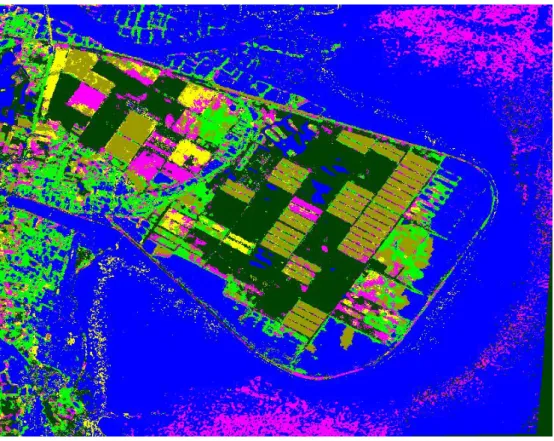
When applied to the first data source (SAR) DL is configured to have 3 input nodes (hh, vv, and hv), 6 output nodes, and 1 hidden layer with 10 hidden nodes. The classification result is shown in Fig. 5 and the classification matrix is given in Table I. It is seen that the overall accuracy is 75.44% and the kappa coefficient is 69.35%. Because that some pixels of the class 4 (rice) are misclassified as class 2 (sugar cane B) and some pixels of the class 3 (basr soil) are misclassified as class 4 (rice) which makes the poor classification accuracy. On the other hand, when applied to the second data source (SPOT) DL is configured to have 3 input nodes (R, G, and IR), 6 output nodes, and 2 hidden layers with 40 hidden nodes each. The classification result is shown in Fig. 6 and the classification matrix is given in Table II. As can be seen, the overall accuracy is 65.01%

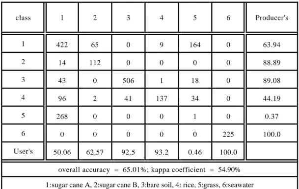
and the kappa coefficient is only 54.90%. The classification accuracy is so low mainly because that some pixels of the class 1 (sugar cane A) are misclassified as class 5 (grass), some pixels of the class 4 (rice) are misclassified as class 1 (sugar cane A), and almost all of the class 5 (grass) are misclassified as class 1 (sugar cane A). Upon applying the variance reduction technique, the classification result is shown in Fig. 7 and the classification matrix is given in Table III.

Part of the class 4 (rice) is misclassified as

(8)

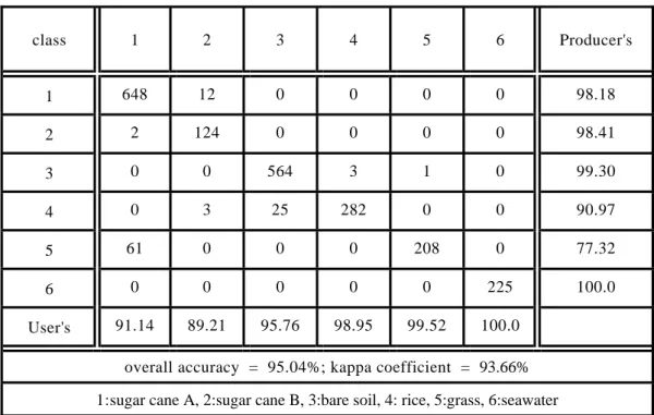
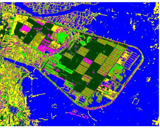
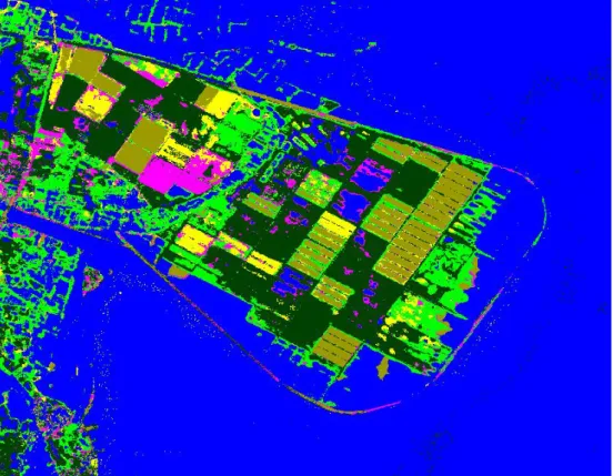
class 2 (sugar cane B). The overall accuracy is 86.75% and the kappa coefficient is 83.21%. The improvement on classification accuracy is not very high may because that the correlation between the outputs of SAR and SPOT is not high enough. On the other hand, when the rms distance weighting policy is applied, the classification result is shown in Fig. 8 and the classification matrix is given in Table IV. The overall accuracy increases up to 95.04% and the kappa coefficient improves dramatically to 93.66%. All of the classes are correctly identified. Also, when the average distance weighting policy is applied, the classification result is shown in Fig. 9 and the classification matrix is given in Table V. The overall accuracy increases up to 95.13% and the kappa coefficient improves dramatically to 93.78%. All of the classes are correctly identified.

5. Conclusions

In this paper, the multiple classifiers approach is utilized for the multisource classification/data fusion to fully utilize the complementary information among different data sources. Three different weighting policies (variance reduction technique, rms distance weighting, and average distance weighting) that are applied to the multiple classifiers approach are introduced. The performances of utilizing the multiple classifiers approach to the application of multisource classification are demonstrated.

Experimental results show that the classification accuracy is dramatically improved by making use of the proposed

method. In addition, both the multiple classifiers that using the rms distance weighting and the average distance weighting outperform that of using variance reduction technique. Moreover, data fusion can take advantage of the use of complementary information to obtain a better overall accuracy than using single data source only.

References

B.V. Dasarthy, 1994. Decision Fusion, IEEE Computer Society Press.

L. Wald, 1999. “Some terms of reference in data fusion,” IEEE Transaction on Geoscience and Remote Sensing, 37, 1190-1193.

J. A. Benediktsson and I. Kanellopoulos, 1999. “Classification of multisource and hyperspectral data based on decision fusion,” IEEE Trans. Geosc. Remote Sensing, 37,1367–1377.

J. A. Benediktsson and Kanellopoulos, I., 1999. “Information extraction based on multisensor data fusion and neural network,” Information Processing for Remote Sensing, 369-395, World Scientific.

S. Gatepaille, Brunessaux, S. Abdulrab, H., 2000. “Data fusion multi-agent framework,” Proceedings of SPIE, 4051, 172-179.

L. A. Gee, and Abidi, M. A., “Multisensor fusion for decision-based control cues,”

Proceedings of SPIE, 4052, 249-257.

Datcu M., Melgani F., Piardi A., and Serpico S. B., 2002. “Multisource data classification with dependence tree.

(9)

IEEE Transaction on Geoscience and Remote Sensing, 40, 609-617.

Briem G. J., Benediktsson J. A., and Sveinsson J. R., 2002. “Multiple classifiers applied to multisource remote sensing data.” IEEE Transaction on Geoscience and Remote Sensing, 31, 801-810.

Serpico S.B. and Roli, F., 1995, Classification of multisensor remote- sensing images by structured neural networks. IEEE Transactions on Geoscience and Remote Sensing , 33, 562 – 578.

Yang-Lang Chang, Chin-Chuan Han, Hsuan Ren, C. T. Chen, K.S. Chen, and Kuo- Chin Fan, 2004. "Data fusion of hyperspectral and SAR images," Optical Engineering, 43(8), 1787–1797.

J. A. Benediktsson, Swain P. H., and Ersoy O.

K., 1990. “Neural network approaches versus statistical methods in classification of multisource remote sensing data,” IEEE Transaction on Geoscience and Remote Sensing, 28, 540-552.

Benediktsson J. A., Sveinsson J. R., Ersoy O.

K., and Swain P. H., 1997. “Parallel consensual neural networks,” IEEE Transaction on Neural Networks, 8, 54- 64.

Benediktsson J. A. and Swain P. H., 1992.

“Consensus theoretic classification methods,” IEEE Transaction on Systems, Man, and Cybernetics, 22, 688-704.

K. Tumer and Ghosh J., 1996. “Analysis of decision boundaries in linearly combined

neural classifiers,” Pattern Recognition, 29, 341-348.

D. H. Wolper, 1992, “Stacked generalization.

Neural Networks, 5, 241-259.

Terry Windeatt, Fabio Roli (Eds.), 2003., Multiple Classifier Systems, 4th International Workshop, MCS 2003, Guilford, UK, June 11-13, 2003, Proceedings. Lecture Notes in Computer Science 2709 Springer 2003, ISBN 3- 540-40369-8.

B. D. Ripley, Pattern Recognition and Neural Networks, 1996., Cambridge University Press.

Y. C. Tzeng, Chen K. S., Kao W. L., and Fung A. K., 1994, “A dynamic learning neural network for remote sensing applications. IEEE Transaction on Geoscience and Remote Sensing,” 32, 1096-1102.

K. S. Chen, Tzeng Y. C., Chen C. F., and Kao W. L., 1995., “Land-cover classification of multispectral imagery using a dynamic learning neural network,” Photogrammetric Engineering and Remote Sensing, 61, 403-408.

K. S. Chen, Huang W. P., Tsay D. H., and Amar F., 1996., “Classification of multifrequency polarimetric SAR imagery using a dynamic learning neural network. IEEE Transaction on Geoscience and Remote Sensing, 34, 814-820.

C. T. Chen, K. S. Chen, and J. S. Lee, 2003.,

“The use of fully polarimetric information for the fuzzy neural classification of SAR images,” IEEE

(10)

Trans. Geoscience and Remote Sensing, 41(9), 2089-2100.

G. A. Carpenter, Gjaja M. N., Gopal S., and Woodcock C. E., 1997., “ART neural networks for remote sensing: vegetation classification from Landsat TM and terrain data,” IEEE Transactions on Geoscience and Remote Sensing, 35 , 308 – 325.

Z. Chair and P. K. Varshney, 1988.

“Distributed Bayesian hypothesis testing with distributed data fusion,” IEEE Trans. Systems, Man, and Cybernetics, 18(5), 695-699.

H. L. Van Trees, 1968, Detection, Estimation and Modulation Theory, vol. 1, New York: John Wiely.

Law A. M. and Kelton W. D., 2^nd ed., 2000.

Simulation Modeling and Analysis, Singapore: McGraw Hill.

S. J. Hook, J. J. Myers, K. J. Thome, M.

Fitzgerald, and A. B. Kahle, 2000, “The modis/aster airborne simulator

~master!—a new instrument for earth science studies,’’ Remote Sens. Environ.

76(1), 93–102.

Table I. Classification Matrix (SAR only)

class 1 2 3 4 5 6 Producer's

1 650 7 2 1 0 0 98.48

2 18 108 0 0 0 0 85.71

3 0 4 294 270 0 0 51.76

4 0 137 8 165 0 0 53.23

5 3 7 52 0 207 0 76.95

6 0 0 16 0 5 204 90.67

User's 96.87 41.06 79.03 37.84 97.64 100.0 overall accuracy = 75.44%; kappa coefficient = 69.35%

1:sugar cane A, 2:sugar cane B, 3:bare soil, 4: rice, 5:grass, 6:seawater

(11)

Table II. Classification Matrix (optical only)

Table III. Classification Matrix (Fusion by variance reduction technique)

1 422 65 0 9 164 0 63.94

2 14 112 0 0 0 0 88.89

3 43 0 506 1 18 0 89.08

4 96 2 41 137 34 0 44.19

5 268 0 0 0 1 0 0.37

6 0 0 0 0 0 225 100.0

1 651 9 0 0 0 0 98.64

2 19 107 0 0 0 0 84.92

3 0 4 518 46 0 0 91.2

4 0 124 2 184 0 0 59.35

5 3 14 63 0 189 0 70.26

6 0 0 2 0 0 223 99.11

User's 96.73 41.47 88.55 80 100.0 100.0 overall accuracy = 86.75%; kappa coefficient = 83.21%

(12)

Table IV. Classification Matrix (Fusion by rms distance weighting)

Table V. Classification Matrix (Fusion by average distance weighting)

1 648 12 0 0 0 0 98.18

2 2 124 0 0 0 0 98.41

3 0 0 564 3 1 0 99.30

4 0 3 25 282 0 0 90.97

5 61 0 0 0 208 0 77.32

6 0 0 0 0 0 225 100.0

class 1 2 3 4 5 6 Producerʹs

1 648 12 0 0 0 0 98.18

2 2 124 0 0 0 0 98.41

3 0 0 564 3 1 0 99.30

4 0 1 30 279 0 0 90.00

5 56 0 0 0 213 0 79.18

6 0 0 0 0 0 225 100.0

Userʹs 91.78 90.51 94.95 98.94 99.53 100.0 overall accuracy = 95.13%; kappa coefficient = 93.78%

(13)

Classifier i

Classifier j Data Source i

Data Source j

Variance Reduction Technique

Winner Takes All X

Y

Xc

Encoded output

Fig.1. Multiple classifiers combined by variance reduction technique

Fig. 2 MASTER images of different bands combination

(14)

Fig. 3. SAR image R:︱HH-VV︱, G:︱HV︳, B:︱HH+VV︳

Fig. 4. Ground truth map of the test site

(15)

Fig. 6. Classification result of (optical only) Fig. 5. Classification result (SAR only)

(16)

Fig. 7. Classification result of (using variance reduction technique)

Fig. 8. Classification result (using rms distance Weighting)

(17)

Fig. 9. Classification result of (using average distance weighting)

(18)

多分類器融合權重分配法之研究

曾裕強

¹

陳錕山

²

摘要

資料融合的關鍵技術之一乃如何有效萃取來自不同感測器的互補資訊。本文即探討利用多分類器系統來達到這個目的。多分類器系統中的必要手段為不同資料來源的權重分配；本文分別提出三種方案:

變異減低法、均方根距離法與平均距離法。實例中我們利用 SAR 影像與光學影像融合於地物分類作為分析評估上述權重分配的性能。結果顯示整體分類精度有大幅度的提升，而三種方案中均方根距離法與平均距離法皆優於變異減低法。

關鍵詞：影像融合、SAR、地物分類、多分類器

收到日期:民國 96 年 05 月 28 日修改日期:民國 96 年 12 月 26 日接受日期:民國 96 年 12 月 27 日

1國立聯合大學電子工程學系教授

2國立中央大學太空及遙測研究中心教授

A New Weighting Scheme with Multiple Classifiers Fusion for Image Classification