Partial remainder

Division

Instructor: Kuan Jen Lin

E-Mail: [email protected] Dept. of EE, FJU, Taiwan Room: SF 727B

Most slides are revision of PowerPoint files

gotten from textbook website.

Division

Chapter 16 Division by Convergence Chapter 15 Variations in Dividers

Chapter 14 High-Radix Dividers

Chapter 13 Basic Division Schemes

Topics in This Part

Review Division schemes and various speedup methods

• Hardest basic operation (fortunately, also the rarest)

• Division speedup methods: high-radix, array, . . .

• Combined multiplication/ division hardware

• Digit-recurrence vs convergence division schemes

13 Basic Division Schemes

Chapter Goals

Study shift/subtract or bit-at-a-time dividers and set the stage for faster methods and variations to be covered in Chapters 14-16

Chapter Highlights

Shift/subtract divide vs shift/add multiply Hardware, firmware, software algorithms Dividing 2’s-complement numbers

The special case of a constant divisor

Shift/Subtract Division Algorithms

Notation for our discussion of division algorithms:

z Dividend z

z

. . . z

z

z

z

d Divisor d

d

. . . d

d

q Quotient q

q

. . . q

q

s Remainder, z – (d × q) s

s

. . . s

s

Initially, we assume unsigned operands

Division of an 8-bit number by a 4-bit number in dot notation.

Dividend Subtracted bit-matrix z

s Remainder

Quotient Divisor q

d

q d 2

–

q d 2

–

q d 2

–

q d 2

–

Division versus Multiplication (1/2)

„ Division is more complex than multiplication:

‰

Need for quotient digit selection or estimation

„ Overflow possibility:

‰

the high-order k bits of z must be strictly less than d; the quotient of a 2k bit number divided by a k bit number may have a width of more than k bits.

Dividend Subtracted bit-matrix z

s Remainder

Quotient Divisor q

d

q d 2 ³ – 3

q d 2 ² – 2

q d 2 ¹ – 1

q d 2 ⁰ – 0

Division versus Multiplication (2/2)

Pentium III latencies

Instruction Latency Cycles/Issue

Load / Store 3 1

Integer Multiply 4 1

Integer Divide 36 36

Double/Single FP Multiply 5 2

Double/Single FP Add 3 1

Double/Single FP Divide 38 38

Division Recurrence

Division with left shifts

s

= 2s

– q

(2

d) with s

= z and

|–shift–| s

= 2

s

|––– subtract –––|

(There is no corresponding right-shift algorithm)

Dividend Subtracted bit-matrix z

s Remainder

Quotient Divisor q

d

q d 2 ₃ ³ –

q d 2 ₂ ² –

q d 2 ₁ ¹ –

q d 2 ₀ ⁰ –

Integer division is characterized by z = d × q + s 2

z = (2

d) × (2

q) + 2

s

z

= d

× q

+ 2

s

Divide fractions like integers; adjust the remainder

No-overflow condition for fractions is:

z

< d

k bits k bits

2z 2

d

0

Division Recurrence Steps

„ Initialization

„ Iterations

‰ One digit arithmetic left-shift of s ^(j) to produce rs ^(j)

‰ Determination of the quotient digit q ^j+1 by the quotient-digit selection function;

„

The index of q could be different

‰ Generation of the divisor multiple d × q ^j+1

‰ Subtraction of dq ^j+1 from rs ^(j) .

‰ On-the-fly conversion of the quotient

„

Or done in the termination step

„ Termination:

‰ make sign(s)=sign(d)), conversion

Examples of Basic Division

Integer division Fractional division

====================== =====================

z 0 1 1 1 0 1 0 1 z

. 0 1 1 1 0 1 0 1

2

d 1 0 1 0 d

. 1 0 1 0

====================== =====================

s

0 1 1 1 0 1 0 1 s

. 0 1 1 1 0 1 0 1 2s

0 1 1 1 0 1 0 1 2s

0 . 1 1 1 0 1 0 1 –q

2

d 1 0 1 0 {q

= 1} –q

d . 1 0 1 0 {q

=1}

––––––––––––––––––––––– ––––––––––––––––––––––

s

0 1 0 0 1 0 1 s

. 0 1 0 0 1 0 1 2s

0 1 0 0 1 0 1 2s

0 . 1 0 0 1 0 1

–q

2

d 0 0 0 0 {q

= 0} –q

d . 0 0 0 0 {q

=0}

––––––––––––––––––––––– ––––––––––––––––––––––

s

1 0 0 1 0 1 s

. 1 0 0 1 0 1 2s

1 0 0 1 0 1 2s

1 . 0 0 1 0 1

–q

2

d 1 0 1 0 {q

= 1} –q

d . 1 0 1 0 {q

=1}

––––––––––––––––––––––– ––––––––––––––––––––––

s

1 0 0 0 1 s

. 1 0 0 0 1 2s

1 0 0 0 1 2s

1 . 0 0 0 1

–q

2

d 1 0 1 0 {q

= 1} –q

d . 1 0 1 0 {q

=1}

––––––––––––––––––––––– ––––––––––––––––––––––

s

0 1 1 1 s

. 0 1 1 1

s 0 1 1 1 s

0 . 0 0 0 0 0 1 1 1

q 1 0 1 1 q

. 1 0 1 1

====================== =====================

Notice the index of q

What is the

residual of

0.0112 / 0.1?

Main Factors Affecting the Overall Execution Time and Cost

„ Radix r

„ Quotient-digit set

‰ Redundant signed digit?

„ Representation of the residual

‰ CSA?

„ Quotient-digit selection

Programmed Division

Register usage for programmed division.

Rs Rq

Rd

0 0 . . . 0 0 0 0 2 d ^k

Carry Flag

Shifted Partial

Remainder Shifted Partial Quotient

Partial Remainder

(2k – j Bits) Partial Quotient (j Bits)

Next quotient digit inserted here

Divisor d

Assembly Language Program for Division

Programmed division using left shifts.

{Using left shifts, divide unsigned 2k-bit dividend,

z_high|z_low, storing the k-bit quotient and remainder.

Registers: R0 holds 0 Rc for counter

Rd for divisor Rs for z_high & remainder Rq for z_low & quotient}

{Load operands into registers Rd, Rs, and Rq}

div: load Rd with divisor load Rs with z_high load Rq with z_low {Check for exceptions}

branch d_by_0 if Rd = R0 branch d_ovfl if Rs > Rd {Initialize counter}

load k into Rc {Begin division loop}

d_loop: shift Rq left 1 {zero to LSB, MSB to carry}

rotate Rs left 1 {carry to LSB, MSB to carry}

skip if carry = 1

branch no_sub if Rs < Rd sub Rd from Rs

incr Rq {set quotient digit to 1}

no_sub: decr Rc {decrement counter by 1}

branch d_loop if Rc 　 0 {Store the quotient and remainder}

store Rq into quotient store Rs into remainder d_by_0: ...

d_ovfl: ...

d_done: ...

Rs Rq

Rd

0 0 . . . 0 0 0 0 2 d^k

Carry Flag

Shifted Partial

Remainder Shifted Partial Quotient

Partial Remainder

(2k ?j Bits) Partial Quotient (j Bits)

Next quotient digit inserted here

Divisor d

Register usage

for programmed

division.

Time Complexity of Programmed Division

Assume k-bit words

k iterations of the main loop

6 or 8 instructions per iteration, depending on the quotient bit

Thus, 6k + 3 to 8k + 3 machine instructions, ignoring operand loads and result store

k = 32 implies 220 ⁺ instructions on average This is too slow for many modern applications!

Microprogrammed division would be somewhat better

Restoring Hardware Dividers

Shift/subtract sequential restoring divider.

Quotient q

Mux

Adder c

0 1

Partial remainder s (initial value z)

Divisor d

Shift Shift

Load

1 c

(j)

Quotient digit selector q

MSB of 2s

k

k

k

Trial difference

Indirect Signed Division

In division with signed operands, q and s are defined by z = d × q + s sign(s) = sign(z) |s | < |d | Examples of division with signed operands

z = 5 d = 3 ⇒ q = 1 s = 2 z = 5 d = –3 ⇒ q = –1 s = 2 z = –5 d = 3 ⇒ q = –1 s = –2 z = –5 d = –3 ⇒ q = 1 s = –2

Magnitudes of q and s are unaffected by input signs Signs of q and s are derivable from signs of z and d Will discuss direct signed division later

(not q = –2, s = –1)

Example of Restoring Unsigned Division

=======================

z 0 1 1 1 0 1 0 1 2

d 0 1 0 1 0

–2

d 1 0 1 1 0

=======================

s

0 0 1 1 1 0 1 0 1 2s

0 1 1 1 0 1 0 1 +(–2

d) 1 0 1 1 0

––––––––––––––––––––––––

s

0 0 1 0 0 1 0 1 Positive, so set q

= 1 2s

0 1 0 0 1 0 1

+(–2

d) 1 0 1 1 0

––––––––––––––––––––––––

s

1 1 1 1 1 0 1 Negative, so set q

= 0 s

=2s

0 1 0 0 1 0 1 and restore

2s

1 0 0 1 0 1 +(–2

d) 1 0 1 1 0

––––––––––––––––––––––––

s

0 1 0 0 0 1 Positive, so set q

= 1 2s

1 0 0 0 1

+(–2

d) 1 0 1 1 0

––––––––––––––––––––––––

s

0 0 1 1 1 Positive, so set q

= 1

s 0 1 1 1

q 1 0 1 1

=======================

No overflow, because

(0111)

< (1010)

Nonrestoring and Signed Division

The cycle time in restoring division must be long enough to allow:

Shifting the registers

Allowing signals to propagate through the adder Determining and storing the next quotient digit Storing the trial difference, if required

Quotient q

Mux

Adder c out

0 1

Partial remainder s (initial value z)

Divisor d

Shift Shift

Load

1 c in

(j)

Quotient digit selector q _k–j

MSB of 2s ^(j–1) k

k k Trial difference

Nonrestoring division to the rescue!

Assume q

= 1 and subtract Store the result as the new PR

(the partial remainder can

become incorrect, hence

the name “nonrestoring”)

Justification for Nonrestoring Division

Why it is acceptable to store an incorrect value in the partial-remainder register?

Shifted partial remainder at start of the cycle is u

Suppose subtraction yields the negative result u – 2

d

Option 1: Restore the partial remainder to correct value u, shift left, and subtract to get 2u – 2

d

Option 2: Keep the incorrect partial remainder u – 2

d,

shift left, and add to get 2(u – 2

d) + 2

d = 2u – 2

d

Example of Nonrestoring Unsigned Division

=======================

z 0 1 1 1 0 1 0 1 2

d 0 1 0 1 0

–2

d 1 0 1 1 0

=======================

s

0 0 1 1 1 0 1 0 1

2s

0 1 1 1 0 1 0 1 Positive, +(–2

d) 1 0 1 1 0 so subtract ––––––––––––––––––––––––

s

0 0 1 0 0 1 0 1

2s

0 1 0 0 1 0 1 Positive, so set q

= 1 +(–2

d) 1 0 1 1 0 and subtract

––––––––––––––––––––––––

s

1 1 1 1 1 0 1

2s

1 1 1 1 0 1 Negative, so set q

= 0 +2

d 0 1 0 1 0 and add

––––––––––––––––––––––––

s

0 1 0 0 0 1

2s

1 0 0 0 1 Positive, so set q

= 1 +(–2

d) 1 0 1 1 0 and subtract

––––––––––––––––––––––––

s

0 0 1 1 1 Positive, so set q

= 1

s 0 1 1 1

q 1 0 1 1

=======================

No overflow: (0111)

< (1010)

Applying “if sign(s) = sign(d) then qk–j = 1 else qk–j = -1 “, we get 11-11, that

equals 1011

Graphical Depiction of Nonrestoring Division

300

200

100

0

–100 117

234

74

148

–12 296

136 272

112

s⁽⁰⁾

s⁽¹⁾

s⁽²⁾

s⁽³⁾

s =16s⁽⁴⁾

2 –160

×

×2 ×2

×2

–160

–160

–160

Partial remainder

(a) Restoring

148

300

200

100

0

–100 117

234

74

148

–12

–24 136

272

112

s⁽⁰⁾

s⁽¹⁾

s⁽²⁾

s⁽³⁾

s =16s⁽⁴⁾

2 –160

×

×2

×2

×2

–160

+160

–160

Partial remainder

(b) Nonrestoring

Example

(0 1 1 1 0 1 0 1)

/ (1 0 1 0)

(117)

/ (10)

Nonrestoring Division with Signed Operands

Restoring division

q

= 0 means no subtraction (or subtraction of 0) q

= 1 means subtraction of d

Nonrestoring division

We always subtract or add

It is as if quotient digits are selected from the set {1, −1}:

1 corresponds to subtraction −1 corresponds to addition Our goal is to end up with a remainder that matches the sign

of the dividend

This idea of trying to match the sign of s with the sign z, leads to a direct signed division algorithm

if sign(s) = sign(d) then q

= 1 else q

= −1

Example: q = . . . 0 0 0 1 . . .

. . . 1

1

1

1 . . .

Quotient Conversion and Final Correction

Partial remainder variation and selected quotient

digits during nonrestoring division with d > 0

d

0

−d

+d

−d

−d

−d +d

+d

×2 ×2

×2

×2

×2

−

1 1

1

1 1 1 z

0 1 0 0 1 1 1 1 0 0 1 1 1 Quotient with digits

1 and 1

Final correction step if sign(s) ≠ sign(z):

Add d to, or subtract d from, s; subtract 1 from, or add 1 to, q

Check: −32 + 16 – 8 – 4 + 2 + 1 = −25 = −64 + 32 + 4 + 2 + 1

Replace

1s with 0s

Shift left, complement MSB, and set LSB to 1 to get the 2’s-complement quotient

1 1 0 1 0 0 0

Example of Nonrestoring Signed Division

========================

z 0 0 1 0 0 0 0 1 2

d 1 1 0 0 1

–2

d 0 0 1 1 1

========================

s

0 0 0 1 0 0 0 0 1

2s

0 0 1 0 0 0 0 1 sign(s

) ≠ sign(d), +2

d 1 1 0 0 1 so set q

=

1 and add ––––––––––––––––––––––––

s

1 1 1 0 1 0 0 1

2s

1 1 0 1 0 0 1 sign(s

) = sign(d),

+(–2

d) 0 0 1 1 1 so set q

= 1 and subtract ––––––––––––––––––––––––

s

0 0 0 0 1 0 1

2s

0 0 0 1 0 1 sign(s

) ≠ sign(d), +2

d 1 1 0 0 1 so set q

=

1 and add ––––––––––––––––––––––––

s

1 1 0 1 1 1

2s

1 0 1 1 1 sign(s

) = sign(d),

+(–2

d) 0 0 1 1 1 so set q

= 1 and subtract ––––––––––––––––––––––––

s

1 1 1 1 0 sign(s

) ≠ sign(z),

+(–2

d) 0 0 1 1 1 so perform corrective subtraction ––––––––––––––––––––––––

s

0 0 1 0 1

s 0 1 0 1

q

1 1

1 1

========================

p = 0 1 0 1 Shift, compl MSB 1 1 0 1 1 Add 1 to correct

1 1 0 0 Check: 33/(−7) = −4

On-The-Fly Conversion

Source: Ercegovac and Lang,

“Digital Arithmetic”, pp. 257

Nonrestoring Hardware Divider

Shift-subtract sequential nonrestoring divider.

Quotient

k

Partial Remainder

Divisor

add/sub

k-bit adder k

c

c

Complement

q

2s (j?) MSB of

Divisor Sign

Complement of

Partial Remainder Sign

Division by Constants

Software and hardware aspects:

As was the case for multiplications by constants, optimizing compilers may replace some divisions by shifts/adds/subs; likewise, in custom VLSI circuits, hardware dividers may be replaced by simpler adders Method 1: Find the reciprocal of the constant and multiply (particularly efficient if several numbers must be divided by the same divisor)

Method 2: Use the property that for each odd integer d, there exists an odd integer m such that d × m = 2 ⁿ – 1; hence, d = (2 ⁿ – 1)/m and

Number of shift-adds required is proportional to log k Multiplication by constant Shift-adds

L ) 2

1 )(

2 1 )(

2 1 2 ( )

2 1 ( 2 1 2

4

2n n

n n

n n

n

zm zm

zm d

z

−

= + + +

= −

= −

Example: Division by a Constant

L ) 2

1 )(

2 1 )(

2 1 ( 2 )

2 1 ( 2 1 2

4

2 n n

n n

n n

n

zm zm

zm d

z _{− − −}

− = + + +

= −

= −

Example: Dividing the number z by 5, assuming 24 bits of precision.

We have d = 5, m = 3, n = 4; 5 × 3 = 2

– 1

Instruction sequence for division by 5

q ← z + z shift-left 1 {3z computed}

q ← q + q shift-right 4 {3z(1 + 2

) computed}

q ← q + q shift-right 8 {3z(1 + 2

)(1 + 2

) computed}

q ← q + q shift-right 16 {3z(1 + 2

)(1 + 2

)(1 + 2

) computed}

q ← q shift-right 4 {3z(1 + 2

)(1 + 2

)(1 + 2

)/16 computed}

L ) 2

1 )(

2 1 )(

2 1 16 ( 3 )

2 1 ( 2

3 1

2 3 5

16 8

4 4

4 4

−

−

− = + − + +

= −

= z − z z

z

5 shifts

4 adds

Preview of Fast Dividers

Like multiplication, there are but two ways to speed it up:

a. Reducing the number of operands (divide in a higher radix) b. Adding them faster (keep partial remainder in carry-save form)

a x

p 2 x a ⁰

0

x a 2 1 ¹

x a 2 ₂ ² 2 ³ x a 3

×

(a) k × k integer multiplication

z

s Di visor q

d

q d 2 ₃ ³ –

q d 2 ₂ ² –

q d 2 ₁ ¹ –

q d 2 ₀ ⁰ –

(b) 2k / k integer di vision

Both (a)

Multiplication and (b) division can be considered as

multioperand

addition problems.

There is one complication that makes division inherently more difficult:

The terms to be subtracted from (added to) the dividend are not known a priori but become known as quotient digits are computed;

quotient digits in turn depend on partial remainders

14 High-Radix Dividers

Chapter Goals

Study techniques that allow us to obtain more than one quotient bit in each cycle (two bits in radix 4, three in radix 8, . . .)

Chapter Highlights

Radix > 2 ⇒ quotient digit selection harder Remedy: redundant quotient representation Carry-save addition reduces cycle time

Implementation methods and tradeoffs

Basics of High-Radix Division

Division with left shifts

s

= r s

– q

(r

d) with s

= z and

|–shift–| s

= r

s

|––– subtract –––|

Dividend z

s Remainder

Quotient Divisor q

d

(q q ) d 4

–

2 tw o

4

d (q q )

–

0 tw o

Radix-4 division in dot notation

k digits k digits

r z q

r

d

0

Examples of High-Radix Division

Radix-4 integer division Radix-10 fractional division

====================== =================

z 0 1 2 3 1 1 2 3 z

. 7 0 0 3

4

d 1 2 0 3 d

. 9 9

====================== =================

s

0 1 2 3 1 1 2 3 s

. 7 0 0 3 4s

0 1 2 3 1 1 2 3 10s

7 . 0 0 3

–q

4

d 0 1 2 0 3 {q

= 1} –q

d 6 . 9 3 {q

= 7}

––––––––––––––––––––––– ––––––––––––––––––

s

0 0 2 2 1 2 3 s

. 0 7 3

4s

0 0 2 2 1 2 3 10s

0 . 7 3

–q

4

d 0 0 0 0 0 {q

= 0} –q

d 0 . 0 0 {q

= 0}

––––––––––––––––––––––– ––––––––––––––––––

s

0 2 2 1 2 3 s

. 7 3

4s

0 2 2 1 2 3 s

. 0 0 7 3

–q

4

d 0 1 2 0 3 {q

= 1} q

. 7 0

––––––––––––––––––––––– =================

s

1 0 0 3 3 4s

1 0 0 3 3

–q

4

d 0 3 0 1 2 {q

= 2}

–––––––––––––––––––––––

s

1 0 2 1

s 1 0 2 1

q 1 0 1 2

======================

Difficulty of Quotient Digit Selection

What is the first quotient digit in the following radix-10 division?

_____________

2 0 4 3 | 1 2 2 5 7 9 6 8

The problem with the pencil-and-paper division algorithm is that there is no room for error in choosing the next quotient digit

In the worst case, all k digits of the divisor and k + 1 digits in the partial remainder are needed to make a correct choice

12 / 2 = 6

122 / 20 = 6

1225 / 204 = 6

12257 / 2043 = 5

Suppose we used the redundant signed digit set [–9, 9] in radix 10

Then, we could choose 6 as the next quotient digit, knowing that we can

recover from an incorrect choice by using negative digits: 5 9 = 6 ^- 1

Radix-2 SRT Division (1/3)

The new partial remainder, s

, as a function of the shifted old partial remainder, 2s

, in radix-2 nonrestoring division.

Algorithm in Ch 13.4

–2d 2d

d

–d

q =–1 q =1

2s

s

–j –j

d –d

s

= 2s

– q

d

with s

= z

s

= 2

s

q

∈ {

1, 1}

„ Robertson’s Diagram

‰

Axes: the shifted residual 2s ^(j–1) and the next residual s ^(j)

‰

It shows the possibilities to choose q and keep the next residual bounded.

„ P-D Diagram

‰

Shifted residual (Partial remainder) vs. divisor

Diagrams for Quotient Selection

–2d 2d d

–d q =–1 q =0

q =1

2s

s

–j

–j –j

–d d

Radix-2 SRT Division (2/3)

q

= 0 requires shifting only, which was faster than shift-and-subtract

But how can you tell if –d ≦ 2s (j-1) < d?

s

= 2s

– q

d with s

= z s

= 2

s

q

∈ {

1, 0, 1}

•Allowing 0 as a quotient digit in nonrestoring Division

q _-j =0 for –d ≦ 2s ^(j-1) < d

–2d 2d d

–d q =–1

q =0

q =1

2s

s

–j

–j

–j

d

–d

–1/2 1/2

–1 1

–1/2 1/2

Radix-2 SRT Division (3/3)

The relationship between new and old partial remainders in radix-2 SRT division.

Comparison with constants −½ and ½ is quite simple 2s ≥ +½ means 2s = (0.1xxxxxxxx)

2s < −½ means 2s = (1.0xxxxxxxx)

If 2s

< ½ then q

= － 1 else if 2s

≧ ½

then q

=1 else q

=0 endif

endif

Radix-2 SRT Division with Variable Shifts

S

is adjusted to be in [-1/2, 1/2/).

We use the comparison constants −½ and ½ for quotient digit selection For 2s ≥ +½ or 2s = (0.1xxxxxxxx)

choose q

= 1

For 2s < −½ or 2s = (1.0xxxxxxxx)

choose q

=

1 Choose q

= 0 in other cases, that is, for:

0 ≤ 2s < +½ or 2s = (0.0xxxxxxxx)

−½ ≤ 2s < 0 or 2s = (1.1xxxxxxxx)

Observation: What happens when the magnitude of 2s is fairly small?

2s = (0.00001xxxx)

2s = (1.1110xxxxx)

Choosing q

= 0 would lead to the same condition in the next step;

generate 5 quotient digits 0 0 0 0 1 Generate 4 quotient digits 0 0 0

1 Use leading 0s or leading 1s detection circuit to determine how many quotient digits can be spewed out at once

Statistically, the average skipping distance will be 2.67 bits

Example Unsigned Radix- 2 SRT Division

========================

z . 0 1 0 0 0 1 0 1 d 0 . 1 0 1 0

–d 1 . 0 1 1 0

========================

s

0 . 0 1 0 0 0 1 0 1

2s

0 . 1 0 0 0 1 0 1 ≥ ½, so set q

= 1 +(−d) 1 . 0 1 1 0 and subtract

––––––––––––––––––––––––

s

1 . 1 1 1 0 1 0 1

2s

1 . 1 1 0 1 0 1 In [−½, ½), so set q

= 0 ––––––––––––––––––––––––

s

= 2s

1 . 1 1 0 1 0 1

2s

1 . 1 0 1 0 1 In [−½, ½), so set q

= 0 ––––––––––––––––––––––––

s

= 2s

0 . 1 0 1 0 1

2s

1 . 0 1 0 1 < −½, so set q

=

1

+d 0 . 1 0 1 0 and add

––––––––––––––––––––––––

s

1 . 1 1 1 1 Negative,

+d 0 . 1 0 1 0 so add to correct ––––––––––––––––––––––––

s

0 . 1 0 0 1

s 0 . 0 0 0 0 0 1 0 1

q 0 . 1 0 0

1 Uncorrected BSD quotient q 0 . 0 1 1 0 Convert and subtract ulp

========================

In [−½, ½), so okay

0.1000

-0.0001

0.0111

-0.0001

0.0110

Using Carry-Save Adders

Constant thresholds used for quotient digit selection in radix-2 division with q

in {–1, 0, 1} .

–2d 2d

d

–d q =–1

q =0 q =1

2s

s

–j

–j

–j

–d d

–1/2 0

Choose –1 Choose 0 Choose 1

–1/0 0/+1

Overlap Overlap

You can choose 0 or 1

in the overlay region

Quotient Digit Selection Based on Truncated PR

Sum part of 2s

: u = (u

u

. u

u

. . .)

Carry part of 2s

: v = (v

v

. v

v

. . .)

Approximation to the partial remainder:

t = u

+ v

{Add the 4 MSBs of u and v}

t := u

+ v

if t < –½

then q

= –1 else if t ≥ 0

then q

= 1 else q

= 0 endif

endif

–2d 2d

d

–d q =–1

q =0 q =1

2s^(j–1) s^(j)

–j

–j

–j

–d d

–1/2 0

Choose –1 Choose 0 Choose 1

–1/0 0/+1

Overlap Overlap

Error in t

„ The 4-bit number t=(t ₁ t ₀ .t _-1 t _-2 ) _2/s0compl can be compared to the constants -1/2 and 0 based on only the three bit

values t ₁ , t ₀ and t _-1 .

„ Regardless of sign, truncating the t _-2 results in the

maximum truncated value being ½ (when the trye carry- in to t _-2 is 1 and t _-2 is 1.).

„ Still in overlay region:

‰

If t < -1/2, the true value of 2s

is guaranteed to be less than 0.

‰

If t < 0, we are guaranteed to have 2s

< ½ ≦ ^d.

Divider with Partial Remainder in Carry-Save Form

Carry v

Mux

Adder

0 1

Divisor d

k k

Carry-save adder Select

q

4 bits Shift left

2s

+ulp for 2’s compl

Sum u

Non0 (enable) Sign

(select) 0, d, or d’

Carry Sum

Why We Cannot Use Carry-Save PR with SRT Division

Overlap regions in radix-2 SRT division.

–2d 2d

d

–d q =–1

q =0

q =1

2s

s

–j

–j

–j

d

–d

1 – d

–1 1

–1/2 1/2

1 – d

The overlay can become arbitrarily small as d

approaches 1.

Choosing the Quotient Digits

A p-d plot for radix-2 division with d ∈ [1/2,1), partial remainder in [–d, d), and quotient digits in [–1, 1].

d p

Infeasible region (p cannot be ≥ 2d)

Infeasible region (p cannot be < −2d)

.100 .101 .110 .111 1.

00.1

00.0

11.1

10.0 10.1 11.0 01.1

01.0

−00.1 −01.0 −01.1 −10.0

d 2d

−2d −d Worst-case error

margin in comparison

Choose 1

Choose −1 Choose 0

−1 1

−1 _max

−1 min

1 _min 1_max

0 _max

0 min

OverlapOverlap

0

Use p-d plot to understand the q selection and derive the

needed precision

(number of bits

to look at).

Design of the Quotient Digit Selection Logic

4-bit adder

Combinational logic

Non0 Sign

Shifted sum = (u

u

. u

u

. . .)

Shifted carry = (v

v

. v

v

. . .)

Approx shifted PR = (t

t

. t

t

)

Non0 = t

′ ∨ t

′ ∨ t

′ = (t

t

t

)′

Sign = t

(t

′ ∨ t

′)

Radix-4 SRT Division

New versus shifted old partial remainder in radix-4 division with q

in [–3, 3].

Radix-4 fractional division with left shifts and q

∈ [–3, 3]

s

= 4 s

– q

d with s

= z and s

= 4

s

|–shift–|

|–– subtract ––|

Two difficulties:

How do you choose from among the 7 possible values for q

? If the choice is +3 or −3, how do you form 3d?

–4d 4d

d

–d

4s

–3 –2 –1 0 +1 +2 +3

s

Building the p-d Plot for Radix-4 Division

A p-d plot for radix-4 SRT division with quotient digit set [–3, 3].

d p

Infeasible region (p cannot be ≥ 4d)

.100 .101 .110 .111

10.1

10.0

01.1

00.0 00.1 01.0 11.1

11.0

d 2d Choose 2

Choose 0 Choose 1

3

1

2 max

2 min

1 min

1 _max

0 max ve O ap rl

0

3d 4d

Choose 3

3 _min

2

ve O arl p

ve O arl p Uncertainty

region Uncertainty

region

Uncertainty region:

because of truncation.

The choice between q=3 or q=2

depends not

only the p but

also on one

bit, d

.

–4d 4d d

–d

4s

–3 –2 –1 0 +1 +2 +3

s

2d/3

–2d/3 8d/3

–8d/3

Restricting the Quotient Digit Set in Radix 4

Fig. 14.13 New versus shifted old partial remainder in radix-4 division with q

in [–2, 2].

Radix-4 fractional division with left shifts and q

∈ [–2, 2]

s

= 4 s

– q

d with s

= z and s

= 4

s

|–shift–|

|–– subtract ––|

For this restriction to be feasible, we must have:

s ∈ [−hd, hd) for some h < 1, and 4hd – 2d ≤ hd

This yields h ≤ 2/3 (choose h = 2/3 to minimize the restriction)

d p

.100 .101 .110 .111

10.1

10.0

01.1

00.0 00.1 01.0 11.1

11.0

Choose 2

Choose 0

Choose 1

1

2 _min

1 _min 2 max

1 max

0 max

0 2

ve O a rl p

ve O a rl p Infeasible region

(p cannot be ≥ 8d/3)

8d/3

5d/3

4d/3 2d/3

d/3

Building the p-d Plot with Restricted Radix-4 Digit Set

A p-d plot for radix-4 SRT division with quotient digit set [–2, 2].

Depends

on d

General High-Radix Dividers

Carry v

CSA tree

Adder Divisor d

k k

Select q

Shift left

2s Sum u

Multiple generation /

selection

Carry Sum

q

. . .

| | d q

or its complement

Process to derive the details:

Radix r

Digit set [–α, α] for q

Number of bits of p (v and u) and d to be inspected

Quotient digit selection unit (table or logic)

Multiple generation/selection scheme

Conversion of redundant q to

2’s complement

15 Variations in Dividers

Chapter Goals

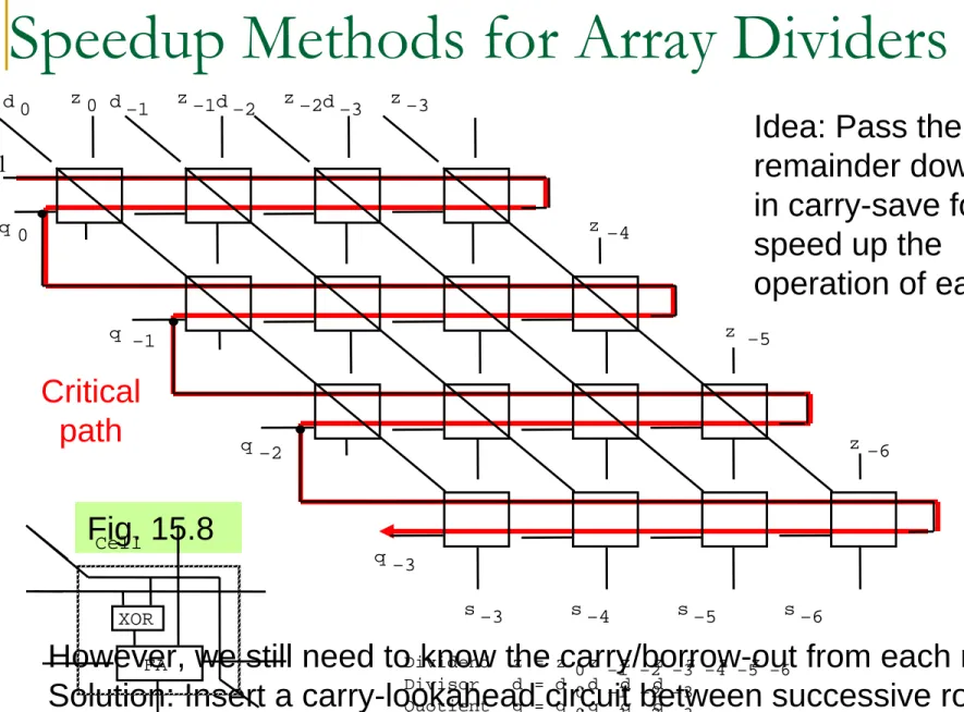
Discuss practical aspects of designing high-radix division schemes and cover other types of fast hardware dividers Chapter Highlights

Building and using p-d plots in practice Prescaling simplifies q digit selection Parallel hardware (array) dividers

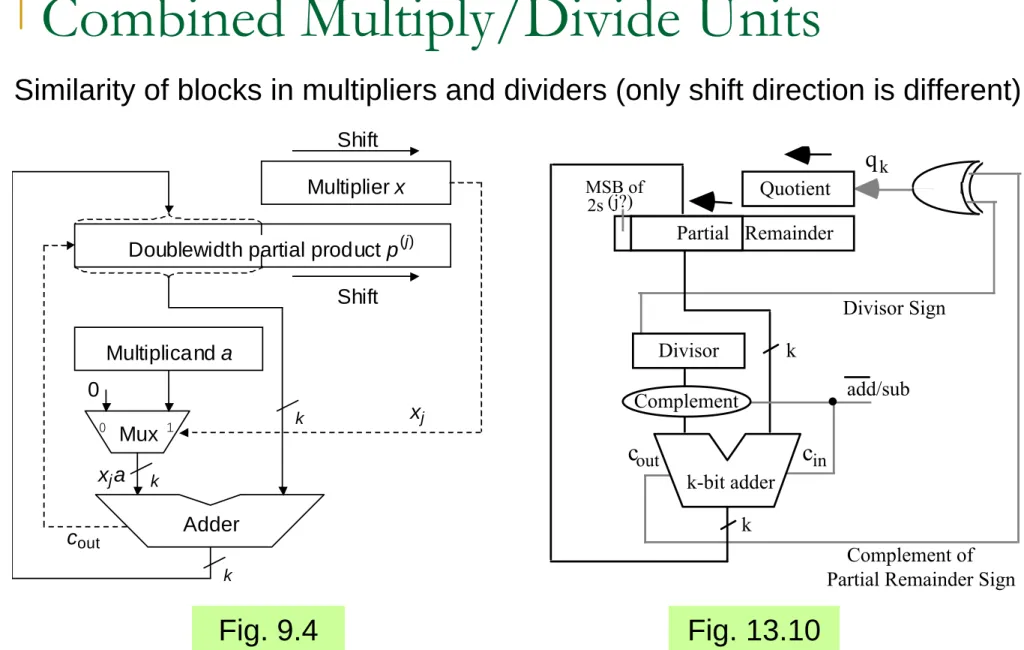
Shared hardware in multipliers/dividers

Square-rooting not special case of division

Quotient Digit Selection Revisited

Radix-r division with quotient digit set [–α, α], α < r – 1 Restrict the partial remainder range, say to [–hd, hd)

From the solid rectangle in Fig. 15.1, we get rhd – αd ≤ hd or h ≤ α/(r – 1) To minimize the range restriction, we choose h = α/(r – 1)

The relationship between new and shifted old partial remainders in radix-r division with quotient digits in [–α, +α].

–α

r s

s

r–1

rhd –rhd

hd

–hd

d

–d

–r+1 –1 0 1 α

rd

–rd – αd d –d 0 αd

Why Using Truncated p and d Values Is Acceptable

A part of p-d plot showing the overlap region for choosing the quotient digit value β or β+1 in radix-r division with quotient digit set [–α, α].

p

d Choose β + 1

Choose β

d ^min

Overlap region

(h + β + 1)d

A

(h + β)d

(–h + β + 1)d (–h + β)d

B

4 bits of p 3 bits of d

3 bits of p 4 bits of d

Note: h = α / (r – 1)

Standard p

xx.xxxx

Carry-save p

xx.xxxxx

xx.xxxxx

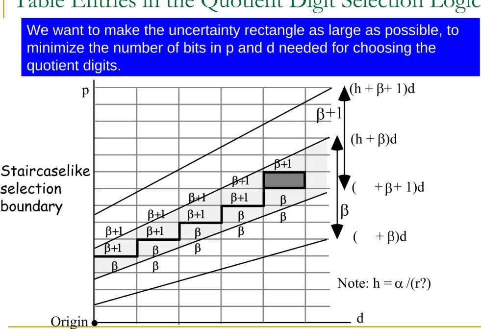
Table Entries in the Quotient Digit Selection Logic

We want to make the uncertainty rectangle as large as possible, to minimize the number of bits in p and d needed for choosing the quotient digits.

p

d

β +1

(h + )d

( + )d 　 (h + + 1)d

( + + 1)d 　

Note: h = /(r?)

β

β

β

β

β α

β

β+1 β

β

β β

β β

β β β+1 β+1

β+1 β+1

β+1 β+1

β+1

β+1 or δ+1 δ

Origin

Staircaselike

selection

boundary

Using p-d Plots in Practice

Establishing upper bounds on the dimensions of uncertainty rectangles.

Δp p

d

Choose α

Choose α − 1

d

Overlap region

(h + α − 1)d

(−h + α)d Δd

d

+ Δd (h + α − 1) d

( −h + α) d

Smallest Δd occurs for the overlap region of α and α – 1

α +

−

= −

Δ h

d h

d _min 2 1

) 1 2

min ( −

=

Δ p d h

Example: Lower Bounds on Precision

) 1 2

min ( −

=

Δ p d h

Fig. 15.4

Δp p

d

Choose α

Choose α − 1

d ^min

Overlap region

(h + α − 1)d

(−h + α)d Δd

d ^min + Δd (h + α − 1) d ^min

(−h + α) d ^min

For r = 4, divisor range [0.5, 1), digit set [–2, 2], we have α = 2, d

= 1/2, h = α/(r – 1) = 2/3

Because 1/8 = 2

and 2

≤ 1/6 < 2

, we must inspect at least 3 bits of d (2, given its leading 1) and 3 bits of p

These are lower bounds (not truncated bits) and may prove inadequate In fact, 3 bits of p and 4 (3) bits of d are required

With p in carry-save form, 4 bits of each component must be inspected

8 / 2 1

3 / 2

1 3 / ) 4 2 / 1

( =

+

−

= −

Δd Δp = ( 1 / 2 )( 4 / 3 − 1 ) = 1 / 6

α +

−

= −

Δ h

d h

d _min 2 1

Upper Bounds for Precision

Theorem: Once lower bounds on precision are determined based on Δd and Δp, one more bit of precision in each direction is always adequate

u Δp v

p

d w

Choose a

Choose a − 1

d

Overlap region

w

(a − 1 + h)d

(a − h)d

Δd A

B

Proof: Let w be the spacing of vertical grid lines

w ≤ Δd/2 ⇒ v ≤ Δp/2 ⇒ u ≥ Δp/2

Some Implementation Details

The asymmetry of quotient digit selection process.

p

d

Choose β + 1

Choose β

d ^min A

B

d ^max

−β β + 1

Choose −β + 1 Choose −β

p

d β

β +1

β β

β β

β

δ β+1 β+1 β

β+1 β+1

β+1

β+1 orδ+1 δ

* *

* *

Example of p-d plot allowing larger uncertainty rectangles, if the 4 cases marked with

asterisks are handled as

exceptions.