Large-Scale Multiprocessors and Scientific Applications

(1)

I.3 Characteristics of Scientific Applications I-6

I.4 Synchronization: Scaling Up I-12

I.5 Performance of Scientific Applications on Shared-Memory

Multiprocessors I-21 I.6 Performance Measurement of Parallel Processors

with Scientific Applications I-33

I.7 Implementing Cache Coherence I-34

I.8 The Custom Cluster Approach: Blue Gene/L I-41

I.9 Concluding Remarks I-44

(2)

I

Large-Scale Multiprocessors and Scientific Applications

¹

Hennessy and Patterson should move MPPs to Chapter 11.

Jim Gray, Microsoft Research when asked about the coverage of massively parallel processors (MPPs) for the third edition in 2000

Unfortunately for companies in the MPP business, the third edition had only ten chapters and the MPP business did not grow as anticipated when the first and second edition were written.

(3)

The primary application of large-scale multiprocessors is for true parallel programming, as opposed to multiprogramming or transaction-oriented computing where independent tasks are executed in parallel without much interaction. In true parallel computing, a set of tasks execute in a collaborative fashion on one application. The primary target of parallel computing is scientific and technical applications. In contrast, for loosely coupled commercial applications, such as Web servers and most transaction-processing applications, there is little communication among tasks. For such applications, loosely coupled clusters are gener- ally adequate and most cost-effective, since intertask communication is rare.

Because true parallel computing involves cooperating tasks, the nature of communication between those tasks and how such communication is supported in the hardware is of vital importance in determining the performance of the application. The next section of this appendix examines such issues and the characteristics of different communication models.

In comparison to sequential programs, whose performance is largely dictated by the cache behavior and issues related to instruction-level parallelism, parallel programs have several additional characteristics that are important to performance, including the amount of parallelism, the size of parallel tasks, the frequency and nature of intertask communication, and the frequency and nature of synchronization. These aspects are affected both by the underlying nature of the application as well as by the programming style. Section I.3 reviews the important characteristics of several scientific applications to give a flavor of these issues.

As we saw in Chapter 5, synchronization can be quite important in achieving good performance. The larger number of parallel tasks that may need to synchronize makes contention involving synchronization a much more serious problem in large-scale multiprocessors. Section I.4 examines methods of scaling up the synchronization mechanisms of Chapter 5.

Section I.5 explores the detailed performance of shared-memory parallel applications executing on a moderate-scale shared-memory multiprocessor. As we will see, the behavior and performance characteristics are quite a bit more complicated than those in small-scale shared-memory multiprocessors. Section I.6 discusses the general issue of how to examine parallel performance for different sized multiprocessors. Section I.7 explores the implementation challenges of distributed shared-memory cache coherence, the key architectural approach used in moderate-scale multiprocessors. Sections I.7 and I.8 rely on a basic understanding of interconnection networks, and the reader should at least quickly review Appendix F before reading these sections.

Section I.8 explores the design of one of the newest and most exciting large- scale multiprocessors in recent times, Blue Gene. Blue Gene is a cluster-based multiprocessor, but it uses a custom, highly dense node designed specifically for this function, as opposed to the nodes of most earlier cluster multiprocessors that used a node architecture similar to those in a desktop or smaller-scale multiprocessor node.

I.1 Introduction

(4)

I.2 Interprocessor Communication: The Critical Performance Issue ■

I-3

By using a custom node design, Blue Gene achieves a significant reduction in the cost, physical size, and power consumption of a node. Blue Gene/L, a 64K-node version, was the world’s fastest computer in 2006, as measured by the linear algebra benchmark, Linpack.

In multiprocessors with larger processor counts, interprocessor communication becomes more expensive, since the distance between processors increases. Fur- thermore, in truly parallel applications where the threads of the application must communicate, there is usually more communication than in a loosely coupled set of distinct processes or independent transactions, which characterize many commercial server applications. These factors combine to make efficient interprocessor communication one of the most important determinants of parallel performance, especially for the scientific market.

Unfortunately, characterizing the communication needs of an application and the capabilities of an architecture is complex. This section examines the key hardware characteristics that determine communication performance, while the next section looks at application behavior and communication needs.

Three performance metrics are critical in any hardware communication mechanism:

1. Communication bandwidth—Ideally, the communication bandwidth is lim- ited by processor, memory, and interconnection bandwidths, rather than by some aspect of the communication mechanism. The interconnection network determines the maximum communication capacity of the system. The bandwidth in or out of a single node, which is often as important as total system bandwidth, is affected both by the architecture within the node and by the communication mechanism. How does the communication mechanism affect the communication bandwidth of a node? When communication occurs, resources within the nodes involved in the communication are tied up or occupied, preventing other outgoing or incoming communication. When this occupancy is incurred for each word of a message, it sets an absolute limit on the communication bandwidth. This limit is often lower than what the network or memory system can provide. Occupancy may also have a component that is incurred for each communication event, such as an incoming or outgoing request. In the latter case, the occupancy limits the communication rate, and the impact of the occupancy on overall communication bandwidth depends on the size of the messages.

2. Communication latency—Ideally, the latency is as low as possible. As Appendix F explains:

Communication latency = Sender overhead + Time of flight + Transmission time + Receiver overhead

I.2 Interprocessor Communication:

The Critical Performance Issue

(5)

assuming no contention. Time of flight is fixed and transmission time is determined by the interconnection network. The software and hardware overheads in sending and receiving messages are largely determined by the communication mechanism and its implementation. Why is latency crucial? Latency affects both performance and how easy it is to program a multiprocessor.

Unless latency is hidden, it directly affects performance either by tying up processor resources or by causing the processor to wait.

Overhead and occupancy are closely related, since many forms of overhead also tie up some part of the node, incurring an occupancy cost, which in turn limits bandwidth. Key features of a communication mechanism may directly affect overhead and occupancy. For example, how is the destination address for a remote communication named, and how is protection implemented? When naming and protection mechanisms are provided by the processor, as in a shared address space, the additional overhead is small.

Alternatively, if these mechanisms must be provided by the operating system for each communication, this increases the overhead and occupancy costs of communication, which in turn reduce bandwidth and increase latency.

3. Communication latency hiding—How well can the communication mecha- nism hide latency by overlapping communication with computation or with other communication? Although measuring this is not as simple as measuring the first two metrics, it is an important characteristic that can be quantified by measuring the running time on multiprocessors with the same communication latency but different support for latency hiding. Although hiding latency is certainly a good idea, it poses an additional burden on the software system and ultimately on the programmer. Furthermore, the amount of latency that can be hidden is application dependent. Thus, it is usually best to reduce latency wherever possible.

Each of these performance measures is affected by the characteristics of the communications needed in the application, as we will see in the next section. The size of the data items being communicated is the most obvious characteristic, since it affects both latency and bandwidth directly, as well as affecting the effi- cacy of different latency-hiding approaches. Similarly, the regularity in the communication patterns affects the cost of naming and protection, and hence the communication overhead. In general, mechanisms that perform well with smaller as well as larger data communication requests, and irregular as well as regular communication patterns, are more flexible and efficient for a wider class of applications. Of course, in considering any communication mechanism, designers must consider cost as well as performance.

Advantages of Different Communication Mechanisms

The two primary means of communicating data in a large-scale multiprocessor are message passing and shared memory. Each of these two primary communication

(6)

I.2 Interprocessor Communication: The Critical Performance Issue ■

I-5

mechanisms has its advantages. For shared-memory communication, the advantages include

■ Compatibility with the well-understood mechanisms in use in centralized multiprocessors, which all use shared-memory communication. The OpenMP consortium (see www.openmp.org for description) has proposed a standard- ized programming interface for shared-memory multiprocessors. Although message passing also uses a standard, MPI or Message Passing Interface, this standard is not used either in shared-memory multiprocessors or in loosely coupled clusters in use in throughput-oriented environments.

■ Ease of programming when the communication patterns among processors are complex or vary dynamically during execution. Similar advantages sim- plify compiler design.

■ The ability to develop applications using the familiar shared-memory model, focusing attention only on those accesses that are performance critical.

■ Lower overhead for communication and better use of bandwidth when communicating small items. This arises from the implicit nature of communication and the use of memory mapping to implement protection in hardware, rather than through the I/O system.

■ The ability to use hardware-controlled caching to reduce the frequency of remote communication by supporting automatic caching of all data, both shared and private. As we will see, caching reduces both latency and contention for accessing shared data. This advantage also comes with a disadvan- tage, which we mention b low.

The major advantages for message-passing communication include the following:

■ The hardware can be simpler, especially by comparison with a scalable shared- memory implementation that supports coherent caching of remote data.

■ Communication is explicit, which means it is simpler to understand. In shared-memory models, it can be difficult to know when communication is occurring and when it is not, as well as how costly the communication is.

■ Explicit communication focuses programmer attention on this costly aspect of parallel computation, sometimes leading to improved structure in a multiprocessor program.

■ Synchronization is naturally associated with sending messages, reducing the possibility for errors introduced by incorrect synchronization.

■ It makes it easier to use sender-initiated communication, which may have some advantages in performance.

■ If the communication is less frequent and more structured, it is easier to improve fault tolerance by using a transaction-like structure. Furthermore, the

e

(7)

less tight coupling of nodes and explicit communication make fault isolation simpler.

■ The very largest multiprocessors use a cluster structure, which is inherently based on message passing. Using two different communication models may introduce more complexity than is warranted.

Of course, the desired communication model can be created in software on top of a hardware model that supports either of these mechanisms. Supporting message passing on top of shared memory is considerably easier: Because messages essentially send data from one memory to another, sending a message can be implemented by doing a copy from one portion of the address space to another. The major difficulties arise from dealing with messages that may be mis- aligned and of arbitrary length in a memory system that is normally oriented toward transferring aligned blocks of data organized as cache blocks. These difficulties can be overcome either with small performance penalties in software or with essentially no penalties, using a small amount of hardware support.

Supporting shared memory efficiently on top of hardware for message passing is much more difficult. Without explicit hardware support for shared memory, all shared-memory references need to involve the operating system to provide address translation and memory protection, as well as to translate memory references into message sends and receives. Loads and stores usually move small amounts of data, so the high overhead of handling these communications in software severely limits the range of applications for which the performance of software-based shared memory is acceptable. For these reasons, it has never been practical to use message passing to implement shared memory for a commercial system.

The primary use of scalable shared-memory multiprocessors is for true parallel programming, as opposed to multiprogramming or transaction-oriented computing. The primary target of parallel computing is scientific and technical applications. Thus, understanding the design issues requires some insight into the behavior of such applications. This section provides such an introduction.

Characteristics of Scientific Applications

Our scientific/technical parallel workload consists of two applications and two computational kernels. The kernels are fast Fourier transformation (FFT) and an LU decomposition, which were chosen because they represent commonly used techniques in a wide variety of applications and have performance characteristics typical of many parallel scientific applications. In addition, the kernels have small code segments whose behavior we can understand and directly track to spe- cific architectural characteristics. Like many scientific applications, I/O is essentially nonexistent in this workload.

I.3 Characteristics of Scientific Applications

(8)

I.3 Characteristics of Scientific Applications ■

I-7

The two applications that we use in this appendix are Barnes and Ocean, which represent two important but very different types of parallel computation.

We briefly describe each of these applications and kernels and characterize their basic behavior in terms of parallelism and communication. We describe how the problem is decomposed for a distributed shared-memory multiprocessor; certain data decompositions that we describe are not necessary on multiprocessors that have a single, centralized memory.

The FFT Kernel

The FFT is the key kernel in applications that use spectral methods, which arise in fields ranging from signal processing to fluid flow to climate modeling. The FFT application we study here is a one-dimensional version of a parallel algo- rithm for a complex number FFT. It has a sequential execution time for n data points of n log n. The algorithm uses a high radix (equal to ) that minimizes communication. The measurements shown in this appendix are collected for a million-point input data set.

There are three primary data structures: the input and output arrays of the data being transformed and the roots of unity matrix, which is precomputed and only read during the execution. All arrays are organized as square matrices. The six steps in the algorithm are as follows:

1. Transpose data matrix.

2. Perform 1D FFT on each row of data matrix.

3. Multiply the roots of unity matrix by the data matrix and write the result in the data matrix.

5. Perform 1D FFT on each row of data matrix.

The data matrices and the roots of unity matrix are partitioned among processors in contiguous chunks of rows, so that each processor’s partition falls in its own local memory. The first row of the roots of unity matrix is accessed heavily by all processors and is often replicated, as we do, during the first step of the algorithm just shown. The data transposes ensure good locality during the individual FFT steps, which would otherwise access nonlocal data.

The only communication is in the transpose phases, which require all-to-all communication of large amounts of data. Contiguous subcolumns in the rows assigned to a processor are grouped into blocks, which are transposed and placed into the proper location of the destination matrix. Every processor transposes one block locally and sends one block to each of the other processors in the system.

Although there is no reuse of individual words in the transpose, with long cache blocks it makes sense to block the transpose to take advantage of the spatial locality afforded by long blocks in the source matrix.

n

(9)

The LU Kernel

LU is an LU factorization of a dense matrix and is representative of many dense linear algebra computations, such as QR factorization, Cholesky factorization, and eigenvalue methods. For a matrix of size n × n the running time is n³ and the parallelism is proportional to n². Dense LU factorization can be performed efficiently by blocking the algorithm, using the techniques in Chapter 2, which leads to highly efficient cache behavior and low communication. After blocking the algorithm, the dominant computation is a dense matrix multiply that occurs in the innermost loop. The block size is chosen to be small enough to keep the cache miss rate low and large enough to reduce the time spent in the less parallel parts of the computation. Relatively small block sizes (8 × 8 or 16 × 16) tend to satisfy both criteria.

Two details are important for reducing interprocessor communication. First, the blocks of the matrix are assigned to processors using a 2D tiling: The (where each block is B × B) matrix of blocks is allocated by laying a grid of size p× p over the matrix of blocks in a cookie-cutter fashion until all the blocks are allocated to a processor. Second, the dense matrix multiplication is performed by the processor that owns the destination block. With this blocking and allocation scheme, communication during the reduction is both regular and predictable. For the measurements in this appendix, the input is a 512 × 512 matrix and a block of 16 × 16 is used.

A natural way to code the blocked LU factorization of a 2D matrix in a shared address space is to use a 2D array to represent the matrix. Because blocks are allocated in a tiled decomposition, and a block is not contiguous in the address space in a 2D array, it is very difficult to allocate blocks in the local memories of the processors that own them. The solution is to ensure that blocks assigned to a processor are allocated locally and contiguously by using a 4D array (with the first two dimensions specifying the block number in the 2D grid of blocks, and the next two specifying the element in the block).

The Barnes Application

Barnes is an implementation of the Barnes-Hut n-body algorithm solving a problem in galaxy evolution. N-body algorithms simulate the interaction among a large number of bodies that have forces interacting among them. In this instance, the bodies represent collections of stars and the force is gravity. To reduce the computational time required to model completely all the individual interactions among the bodies, which grow as n², n-body algorithms take advan- tage of the fact that the forces drop off with distance. (Gravity, for example, drops off as 1/d², where d is the distance between the two bodies.) The Barnes- Hut algorithm takes advantage of this property by treating a collection of bodies that are “far away” from another body as a single point at the center of mass of the collection and with mass equal to the collection. If the body is far enough from any body in the collection, then the error introduced will be negligible. The

n B--- n

B---

×

(10)

I-9

collections are structured in a hierarchical fashion, which can be represented in a tree. This algorithm yields an n log n running time with parallelism proportional to n.

The Barnes-Hut algorithm uses an octree (each node has up to eight children) to represent the eight cubes in a portion of space. Each node then represents the collection of bodies in the subtree rooted at that node, which we call a cell.

Because the density of space varies and the leaves represent individual bodies, the depth of the tree varies. The tree is traversed once per body to compute the net force acting on that body. The force calculation algorithm for a body starts at the root of the tree. For every node in the tree it visits, the algorithm determines if the center of mass of the cell represented by the subtree rooted at the node is “far enough away” from the body. If so, the entire subtree under that node is approxi- mated by a single point at the center of mass of the cell, and the force that this center of mass exerts on the body is computed. On the other hand, if the center of mass is not far enough away, the cell must be “opened” and each of its subtrees visited. The distance between the body and the cell, together with the error toler- ances, determines which cells must be opened. This force calculation phase dom- inates the execution time. This appendix takes measurements using 16K bodies;

the criterion for determining whether a cell needs to be opened is set to the mid- dle of the range typically used in practice.

Obtaining effective parallel performance on Barnes-Hut is challenging because the distribution of bodies is nonuniform and changes over time, making partitioning the work among the processors and maintenance of good locality of reference difficult. We are helped by two properties: (1) the system evolves slowly, and (2) because gravitational forces fall off quickly, with high probability, each cell requires touching a small number of other cells, most of which were used on the last time step. The tree can be partitioned by allocating each processor a subtree. Many of the accesses needed to compute the force on a body in the subtree will be to other bodies in the subtree. Since the amount of work associated with a subtree varies (cells in dense portions of space will need to access more cells), the size of the subtree allocated to a processor is based on some mea- sure of the work it has to do (e.g., how many other cells it needs to visit), rather than just on the number of nodes in the subtree. By partitioning the octree repre- sentation, we can obtain good load balance and good locality of reference, while keeping the partitioning cost low. Although this partitioning scheme results in good locality of reference, the resulting data references tend to be for small amounts of data and are unstructured. Thus, this scheme requires an efficient implementation of shared-memory communication.

The Ocean Application

Ocean simulates the influence of eddy and boundary currents on large-scale flow in the ocean. It uses a restricted red-black Gauss-Seidel multigrid technique to solve a set of elliptical partial differential equations. Red-black Gauss-Seidel is an iteration technique that colors the points in the grid so as to consistently

(11)

update each point based on previous values of the adjacent neighbors. Multigrid methods solve finite difference equations by iteration using hierarchical grids.

Each grid in the hierarchy has fewer points than the grid below and is an approx- imation to the lower grid. A finer grid increases accuracy and thus the rate of con- vergence, while requiring more execution time, since it has more data points.

Whether to move up or down in the hierarchy of grids used for the next iteration is determined by the rate of change of the data values. The estimate of the error at every time step is used to decide whether to stay at the same grid, move to a coarser grid, or move to a finer grid. When the iteration converges at the finest level, a solution has been reached. Each iteration has n²work for ann×n grid and the same amount of parallelism.

The arrays representing each grid are dynamically allocated and sized to the particular problem. The entire ocean basin is partitioned into square subgrids (as close as possible) that are allocated in the portion of the address space corresponding to the local memory of the individual processors, which are assigned responsibility for the subgrid. For the measurements in this appendix we use an input that has 130 × 130 grid points. There are five steps in a time iteration. Since data are exchanged between the steps, all the processors present synchronize at the end of each step before proceeding to the next. Communication occurs when the boundary points of a subgrid are accessed by the adjacent subgrid in nearest- neighbor fashion.

Computation/Communication for the Parallel Programs

A key characteristic in determining the performance of parallel programs is the ratio of computation to communication. If the ratio is high, it means the application has lots of computation for each datum communicated. As we saw in Section I.2, communication is the costly part of parallel computing; therefore, high computation-to-communication ratios are very beneficial. In a parallel processing environment, we are concerned with how the ratio of computation to communication changes as we increase either the number of processors, the size of the problem, or both. Knowing how the ratio changes as we increase the processor count sheds light on how well the application can be sped up. Because we are often interested in running larger problems, it is vital to understand how changing the data set size affects this ratio.

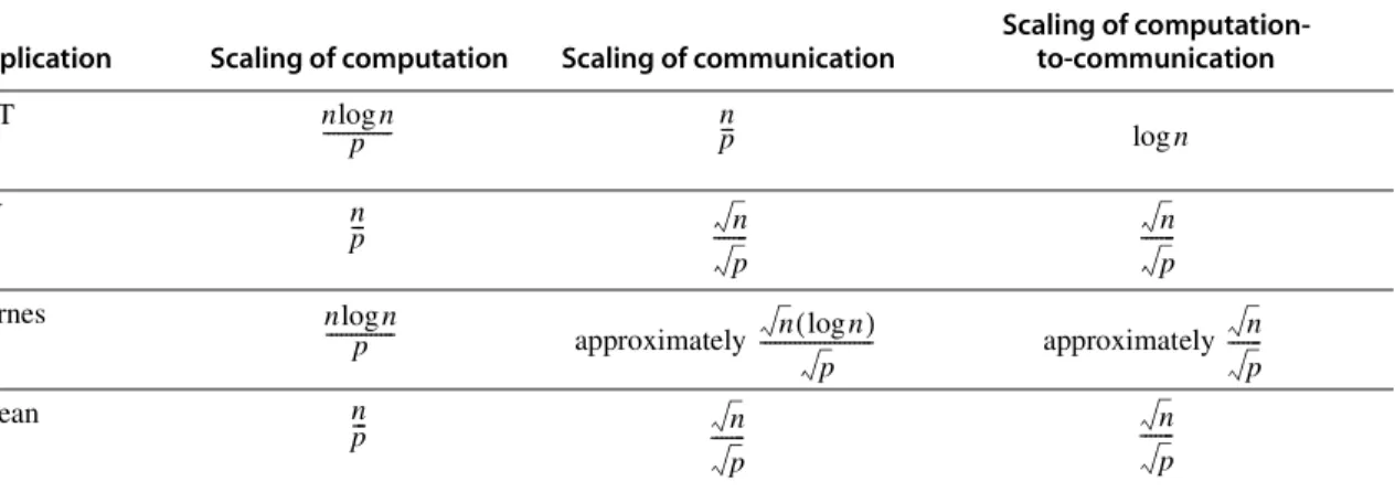
To understand what happens quantitatively to the computation-to-communication ratio as we add processors, consider what happens separately to computation and to communication as we either add processors or increase problem size. Figure I.1 shows that as we add processors, for these applications, the amount of computation per processor falls proportionately and the amount of communication per processor falls more slowly. As we increase the problem size, the computation scales as the O( ) complexity of the algorithm dictates. Communication scaling is more complex and depends on details of the algorithm; we describe the basic phenomena for each application in the caption of Figure I.1.

(12)

I-11

The overall computation-to-communication ratio is computed from the individual growth rate in computation and communication. In general, this ratio rises slowly with an increase in dataset size and decreases as we add processors. This reminds us that performing a fixed-size problem with more processors leads to increasing inefficiencies because the amount of communication among processors grows. It also tells us how quickly we must scale dataset size as we add processors to keep the fraction of time in communication fixed. The following example illustrates these trade-offs.

Example Suppose we know that for a given multiprocessor the Ocean application spends 20% of its execution time waiting for communication when run on four processors.

Assume that the cost of each communication event is independent of processor count, which is not true in general, since communication costs rise with processor count. How much faster might we expect Ocean to run on a 32-processor machine with the same problem size? What fraction of the execution time is spent on communication in this case? How much larger a problem should we run if we want the fraction of time spent communicating to be the same?

Answer The computation-to-communication ratio for Ocean is , so if the problem size is the same, the communication frequency scales by . This means that communication time increases by . We can use a variation on Amdahl’s law, Application Scaling of computation Scaling of communication

Scaling of computation- to-communication FFT

LU

Barnes

approximately approximately Ocean

Figure I.1 Scaling of computation, of communication, and of the ratio are critical factors in determining perfor- mance on parallel multiprocessors. In this table, p is the increased processor count and n is the increased dataset size. Scaling is on a per-processor basis. The computation scales up with n at the rate given by O( ) analysis and scales down linearly as p is increased. Communication scaling is more complex. In FFT, all data points must interact, so com- munication increases with n and decreases with p. In LU and Ocean, communication is proportional to the boundary of a block, so it scales with dataset size at a rate proportional to the side of a square with n points, namely, ; for the same reason communication in these two applications scales inversely to . Barnes has the most complex scaling properties. Because of the fall-off of interaction between bodies, the basic number of interactions among bodies that require communication scales as . An additional factor of log n is needed to maintain the relationships among the bodies. As processor count is increased, communication scales inversely to .

nlogn

---p n

p--- logn

n

p--- n

p

--- n

p --- nlogn

---p n(logn) p

--- n

p --- n

p--- n

p

--- n

p ---

n p

n

p

n

⁄

p p 8

(13)

recognizing that the computation is decreased but the communication time is increased. If T₄ is the total execution time for four processors, then the execution time for 32 processors is

Hence, the speedup is

and the fraction of time spent in communication goes from 20% to 0.57/0.67 = 85%.

For the fraction of the communication time to remain the same, we must keep the computation-to-communication ratio the same, so the problem size must scale at the same rate as the processor count. Notice that, because we have changed the problem size, we cannot fairly compare the speedup of the original problem and the scaled problem. We will return to the critical issue of scaling applications for multiprocessors in Section I.6.

In this section, we focus first on synchronization performance problems in larger multiprocessors and then on solutions for those problems.

Synchronization Performance Challenges

To understand why the simple spin lock scheme presented in Chapter 5 does not scale well, imagine a large multiprocessor with all processors contending for the same lock. The directory or bus acts as a point of serialization for all the processors, leading to lots of contention, as well as traffic. The following example shows how bad things can be.

Example Suppose there are 10 processors on a bus and each tries to lock a variable simultaneously. Assume that each bus transaction (read miss or write miss) is 100 clock cycles long. You can ignore the time of the actual read or write of a lock held in the cache, as well as the time the lock is held (they won’t matter much!).

Determine the number of bus transactions required for all 10 processors to acquire the lock, assuming they are all spinning when the lock is released at time 0. About how long will it take to process the 10 requests? Assume that the bus is

T₃₂ = Compute time + Communication time 0.8×T4

---8 +(0.2×T₄)× 8

=

0.1×T₄+0.57×T₄

= = 0.67×T₄

Speedup T₄ T₃₂

--- T₄ 0.67×T4

--- 1.49

= = =

I.4 Synchronization: Scaling Up

(14)

I.4 Synchronization: Scaling Up ■

I-13

totally fair so that every pending request is serviced before a new request and that the processors are equally fast.

Answer When i processes are contending for the lock, they perform the following sequence of actions, each of which generates a bus transaction:

i load linked operations to access the lock

i store conditional operations to try to lock the lock 1 store (to release the lock)

Thus, for i processes, there are a total of 2i + 1 bus transactions. Note that this assumes that the critical section time is negligible, so that the lock is released before any other processors whose store conditional failed attempt another load linked.

Thus, for n processes, the total number of bus operations is

For 10 processes there are 120 bus transactions requiring 12,000 clock cycles or 120 clock cycles per lock acquisition!

The difficulty in this example arises from contention for the lock and serialization of lock access, as well as the latency of the bus access. (The fairness property of the bus actually makes things worse, since it delays the processor that claims the lock from releasing it; unfortunately, for any bus arbitration scheme some worst-case scenario does exist.) The key advantages of spin locks—that they have low overhead in terms of bus or network cycles and offer good performance when locks are reused by the same processor—are both lost in this example. We will consider alternative implementations in the next section, but before we do that, let’s consider the use of spin locks to implement another common high-level synchronization primitive.

Barrier Synchronization

One additional common synchronization operation in programs with parallel loops is a barrier. A barrier forces all processes to wait until all the processes reach the barrier and then releases all of the processes. A typical implementation of a barrier can be done with two spin locks: one to protect a counter that tallies the processes arriving at the barrier and one to hold the processes until the last process arrives at the barrier. To implement a barrier, we usually use the ability to spin on a variable until it satisfies a test; we use the notation spin(condition) to indicate this. Figure I.2 is a typical implementation, assuming that lock and unlock provide basic spin locks and total is the number of processes that must reach the barrier.

2i+1

( )

i 1=

∑

n ⁼ ^{n n}⁽ ⁺¹^{) n}⁺ ⁼ ⁿ²⁺²ⁿ

(15)

In practice, another complication makes barrier implementation slightly more complex. Frequently a barrier is used within a loop, so that processes released from the barrier would do some work and then reach the barrier again. Assume that one of the processes never actually leaves the barrier (it stays at the spin operation), which could happen if the OS scheduled another process, for example. Now it is possible that one process races ahead and gets to the barrier again before the last process has left. The “fast” process then traps the remaining

“slow” process in the barrier by resetting the flag release. Now all the processes will wait infinitely at the next instance of this barrier because one process is trapped at the last instance, and the number of processes can never reach the value of total.

The important observation in this example is that the programmer did nothing wrong. Instead, the implementer of the barrier made some assumptions about for- ward progress that cannot be assumed. One obvious solution to this is to count the processes as they exit the barrier (just as we did on entry) and not to allow any process to reenter and reinitialize the barrier until all processes have left the prior instance of this barrier. This extra step would significantly increase the latency of the barrier and the contention, which as we will see shortly are already large. An alternative solution is a sense-reversing barrier, which makes use of a private per-process variable, local_sense, which is initialized to 1 for each process.

Figure I.3 shows the code for the sense-reversing barrier. This version of a barrier is safely usable; as the next example shows, however, its performance can still be quite poor.

lock (counterlock);/* ensure update atomic */

if (count==0) release=0;/* first=>reset release */

count = count + 1;/* count arrivals */

unlock(counterlock);/* release lock */

if (count==total) {/* all arrived */

count=0;/* reset counter */

release=1;/* release processes */

}

else {/* more to come */

spin (release==1);/* wait for arrivals */

}

Figure I.2 Code for a simple barrier. The lock counterlock protects the counter so that it can be atomically incremented. The variable count keeps the tally of how many processes have reached the barrier. The variable release is used to hold the processes until the last one reaches the barrier. The operation spin (release==1) causes a process to wait until all processes reach the barrier.

(16)

I-15

Example Suppose there are 10 processors on a bus and each tries to execute a barrier simultaneously. Assume that each bus transaction is 100 clock cycles, as before.

You can ignore the time of the actual read or write of a lock held in the cache as the time to execute other nonsynchronization operations in the barrier implementation. Determine the number of bus transactions required for all 10 processors to reach the barrier, be released from the barrier, and exit the barrier. Assume that the bus is totally fair, so that every pending request is serviced before a new request and that the processors are equally fast. Don’t worry about counting the processors out of the barrier. How long will the entire process take?

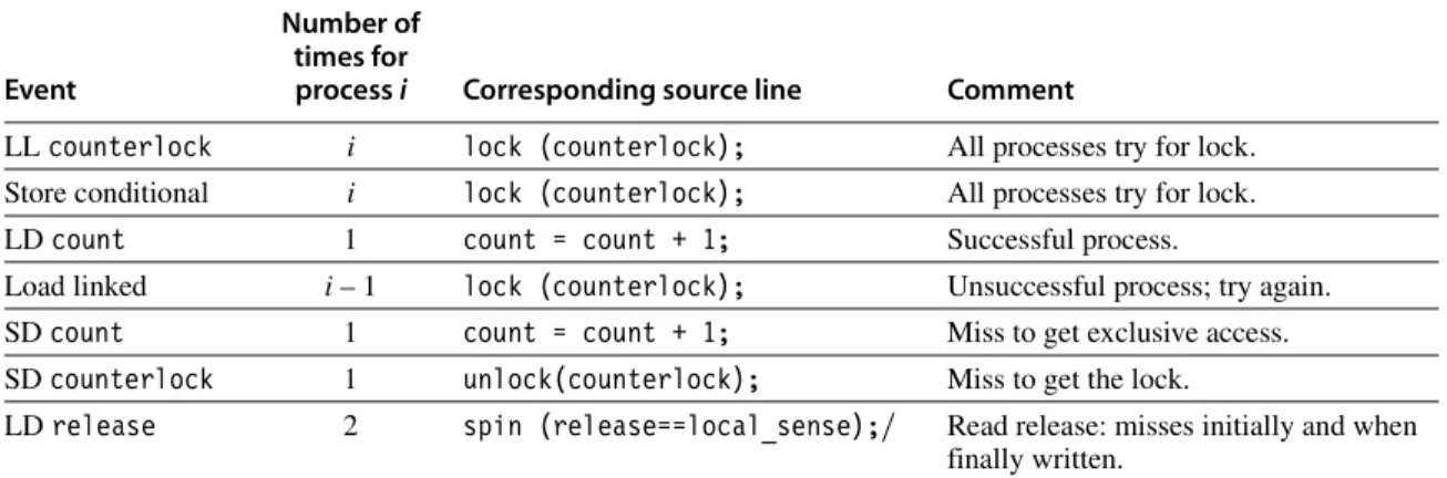
Answer We assume that load linked and store conditional are used to implement lock and unlock. Figure I.4 shows the sequence of bus events for a processor to traverse the barrier, assuming that the first process to grab the bus does not have the lock.

There is a slight difference for the last process to reach the barrier, as described in the caption.

For the ith process, the number of bus transactions is 3i + 4. The last process to reach the barrier requires one less. Thus, for n processes, the number of bus transactions is

For 10 processes, this is 204 bus cycles or 20,400 clock cycles! Our barrier operation takes almost twice as long as the 10-processor lock-unlock sequence.

local_sense =! local_sense; /* toggle local_sense */

lock (counterlock);/* ensure update atomic */

count=count+1;/* count arrivals */

if (count==total) {/* all arrived */

release=local_sense;/* release processes */

}

unlock (counterlock);/* unlock */

spin (release==local_sense);/* wait for signal */

}

Figure I.3 Code for a sense-reversing barrier. The key to making the barrier reusable is the use of an alternating pattern of values for the flag release, which controls the exit from the barrier. If a process races ahead to the next instance of this barrier while some other processes are still in the barrier, the fast process cannot trap the other processes, since it does not reset the value of release as it did in Figure I.2.

3i+4

( )

i 1=

∑

n

⎝ ⎠

⎜ ⎟

⎛ ⎞

1

– 3n²+11n ---2 –1

=

(17)

As we can see from these examples, synchronization performance can be a real bottleneck when there is substantial contention among multiple processes.

When there is little contention and synchronization operations are infrequent, we are primarily concerned about the latency of a synchronization primitive—that is, how long it takes an individual process to complete a synchronization operation.

Our basic spin lock operation can do this in two bus cycles: one to initially read the lock and one to write it. We could improve this to a single bus cycle by a variety of methods. For example, we could simply spin on the swap operation. If the lock were almost always free, this could be better, but if the lock were not free, it would lead to lots of bus traffic, since each attempt to lock the variable would lead to a bus cycle. In practice, the latency of our spin lock is not quite as bad as we have seen in this example, since the write miss for a data item present in the cache is treated as an upgrade and will be cheaper than a true read miss.

The more serious problem in these examples is the serialization of each process’s attempt to complete the synchronization. This serialization is a problem when there is contention because it greatly increases the time to complete the synchronization operation. For example, if the time to complete all 10 lock and unlock operations depended only on the latency in the uncontended case, then it would take 1000 rather than 15,000 cycles to complete the synchronization operations. The barrier situation is as bad, and in some ways worse, since it is highly likely to incur contention. The use of a bus interconnect exacerbates these problems, but serialization could be just as serious in a directory-based multiprocessor, where the latency would be large. The next subsection presents some solutions that are useful when either the contention is high or the processor count is large.

Event

Number of times for

process i Corresponding source line Comment

LL counterlock i lock (counterlock); All processes try for lock.

Store conditional i lock (counterlock); All processes try for lock.

LD count 1 count = count + 1; Successful process.

Load linked i – 1 lock (counterlock); Unsuccessful process; try again.

SD count 1 count = count + 1; Miss to get exclusive access.

SD counterlock 1 unlock(counterlock); Miss to get the lock.

LD release 2 spin (release==local_sense);/ Read release: misses initially and when finally written.

Figure I.4 Here are the actions, which require a bus transaction, taken when the ith process reaches the barrier.

The last process to reach the barrier requires one less bus transaction, since its read of release for the spin will hit in the cache!

(18)

I-17

Synchronization Mechanisms for Larger-Scale Multiprocessors

What we would like are synchronization mechanisms that have low latency in uncontended cases and that minimize serialization in the case where contention is significant. We begin by showing how software implementations can improve the performance of locks and barriers when contention is high; we then explore two basic hardware primitives that reduce serialization while keeping latency low.

Software Implementations

The major difficulty with our spin lock implementation is the delay due to contention when many processes are spinning on the lock. One solution is to artifi- cially delay processes when they fail to acquire the lock. The best performance is obtained by increasing the delay exponentially whenever the attempt to acquire the lock fails. Figure I.5 shows how a spin lock with exponential back-off is implemented. Exponential back-off is a common technique for reducing contention in shared resources, including access to shared networks and buses (see Sec- tions F.4 to F.8). This implementation still attempts to preserve low latency when contention is small by not delaying the initial spin loop. The result is that if many processes are waiting, the back-off does not affect the processes on their first attempt to acquire the lock. We could also delay that process, but the result would

DADDUI R3,R0,#1 ;R3 = initial delay

lockit: LL R2,0(R1) ;load linked

BNEZ R2,lockit ;not available-spin DADDUI R2,R2,#1 ;get locked value

SC R2,0(R1) ;store conditional

BNEZ R2,gotit ;branch if store succeeds DSLL R3,R3,#1 ;increase delay by factor of 2

PAUSE R3 ;delays by value in R3

J lockit

gotit: use data protected by lock

Figure I.5 A spin lock with exponential back-off. When the store conditional fails, the process delays itself by the value in R3. The delay can be implemented by decrement- ing a copy of the value in R3 until it reaches 0. The exact timing of the delay is multiprocessor dependent, although it should start with a value that is approximately the time to perform the critical section and release the lock. The statement pause R3 should cause a delay of R3 of these time units. The value in R3 is increased by a factor of 2 every time the store conditional fails, which causes the process to wait twice as long before trying to acquire the lock again. The small variations in the rate at which competing processors execute instructions are usually sufficient to ensure that processes will not continually collide. If the natural perturbation in execution time was insufficient, R3 could be initialized with a small random value, increasing the variance in the successive delays and reducing the probability of successive collisions.

(19)

be poorer performance when the lock was in use by only two processes and the first one happened to find it locked.

Another technique for implementing locks is to use queuing locks. Queuing locks work by constructing a queue of waiting processors; whenever a processor frees up the lock, it causes the next processor in the queue to attempt access. This eliminates contention for a lock when it is freed. We show how queuing locks operate in the next section using a hardware implementation, but software implementations using arrays can achieve most of the same benefits. Before we look at hardware primitives, let’s look at a better mechanism for barriers.

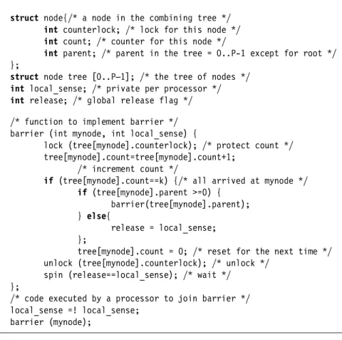
Our barrier implementation suffers from contention both during the gather stage, when we must atomically update the count, and at the release stage, when all the processes must read the release flag. The former is more serious because it requires exclusive access to the synchronization variable and thus creates much more serialization; in comparison, the latter generates only read contention. We can reduce the contention by using a combining tree, a structure where multiple requests are locally combined in tree fashion. The same combining tree can be used to implement the release process, reducing the contention there.

Our combining tree barrier uses a predetermined n-ary tree structure. We use the variable k to stand for the fan-in; in practice, k = 4 seems to work well. When the kth process arrives at a node in the tree, we signal the next level in the tree.

When a process arrives at the root, we release all waiting processes. As in our earlier example, we use a sense-reversing technique. A tree-based barrier, as shown in Figure I.6, uses a tree to combine the processes and a single signal to release the barrier. Some MPPs (e.g., the T3D and CM-5) have also included hardware support for barriers, but more recent machines have relied on software libraries for this support.

Hardware Primitives

In this subsection, we look at two hardware synchronization primitives. The first primitive deals with locks, while the second is useful for barriers and a number of other user-level operations that require counting or supplying distinct indices. In both cases, we can creat a hardware primitive where latency is essentially identi- cal to our earlier version, but with much less serialization, leading to better scaling when there is contention.

The major problem with our original lock implementation is that it introduces a large amount of unneeded contention. For example, when the lock is released all processors generate both a read and a write miss, although at most one processor can successfully get the lock in the unlocked state. This sequence happens on each of the 10 lock/unlock sequences, as we saw in the example on page I-12.

We can improve this situation by explicitly handing the lock from one waiting processor to the next. Rather than simply allowing all processors to compete every time the lock is released, we keep a list of the waiting processors and hand the lock to one explicitly, when its turn comes. This sort of mechanism has been called a queuing lock. Queuing locks can be implemented either in hardware, which we

e

(20)

I-19

describe here, or in software using an array to keep track of the waiting processes.

The basic concepts are the same in either case. Our hardware implementation assumes a directory-based multiprocessor where the individual processor caches are addressable. In a bus-based multiprocessor, a software implementation would be more appropriate and would have each processor using a different address for the lock, permitting the explicit transfer of the lock from one process to another.

How does a queuing lock work? On the first miss to the lock variable, the miss is sent to a synchronization controller, which may be integrated with the memory controller (in a bus-based system) or with the directory controller. If the lock is free, it is simply returned to the processor. If the lock is unavailable,

struct node{/* a node in the combining tree */

int counterlock; /* lock for this node */

int count; /* counter for this node */

int parent; /* parent in the tree = 0..P-1 except for root */

};

struct node tree [0..P–1]; /* the tree of nodes */

int local_sense; /* private per processor */

int release; /* global release flag */

/* function to implement barrier */

barrier (int mynode, int local_sense) {

lock (tree[mynode].counterlock); /* protect count */

tree[mynode].count=tree[mynode].count+1;

/* increment count */

if (tree[mynode].count==k) {/* all arrived at mynode */

if (tree[mynode].parent >=0) { barrier(tree[mynode].parent);

} else{

release = local_sense;

};

tree[mynode].count = 0; /* reset for the next time */

unlock (tree[mynode].counterlock); /* unlock */

spin (release==local_sense); /* wait */

};

/* code executed by a processor to join barrier */

local_sense =! local_sense;

barrier (mynode);

Figure I.6 An implementation of a tree-based barrier reduces contention consider- ably. The tree is assumed to be prebuilt statically using the nodes in the array tree.

Each node in the tree combines k processes and provides a separate counter and lock, so that at most k processes contend at each node. When the kth process reaches a node in the tree, it goes up to the parent, incrementing the count at the parent.

When the count in the parent node reaches k, the release flag is set. The count in each node is reset by the last process to arrive. Sense-reversing is used to avoid races as in the simple barrier. The value of tree[root].parent should be set to –1 when the tree is initially built.

(21)

the controller creates a record of the node’s request (such as a bit in a vector) and sends the processor back a locked value for the variable, which the processor then spins on. When the lock is freed, the controller selects a processor to go ahead from the list of waiting processors. It can then either update the lock variable in the selected processor’s cache or invalidate the copy, causing the processor to miss and fetch an available copy of the lock.

Example How many bus transactions and how long does it take to have 10 processors lock and unlock the variable using a queuing lock that updates the lock on a miss?

Make the other assumptions about the system the same as those in the earlier example on page I-12.

Answer For n processors, each will initially attempt a lock access, generating a bus trans- action; one will succeed and free up the lock, for a total of n + 1 transactions for the first processor. Each subsequent processor requires two bus transactions, one to receive the lock and one to free it up. Thus, the total number of bus transac- tions is (n + 1) + 2(n – 1) = 3n – 1. Note that the number of bus transactions is now linear in the number of processors contending for the lock, rather than qua- dratic, as it was with the spin lock we examined earlier. For 10 processors, this requires 29 bus cycles or 2900 clock cycles.

There are a couple of key insights in implementing such a queuing lock capa- bility. First, we need to be able to distinguish the initial access to the lock, so we can perform the queuing operation, and also the lock release, so we can provide the lock to another processor. The queue of waiting processes can be implemented by a variety of mechanisms. In a directory-based multiprocessor, this queue is akin to the sharing set, and similar hardware can be used to implement the directory and queuing lock operations. One complication is that the hardware must be prepared to reclaim such locks, since the process that requested the lock may have been context-switched and may not even be scheduled again on the same processor.

Queuing locks can be used to improve the performance of our barrier operation. Alternatively, we can introduce a primitive that reduces the amount of time needed to increment the barrier count, thus reducing the serialization at this bottleneck, which should yield comparable performance to using queuing locks. One primitive that has been introduced for this and for building other synchronization operations is fetch-and-increment, which atomically fetches a variable and incre- ments its value. The returned value can be either the incremented value or the fetched value. Using fetch-and-increment we can dramatically improve our barrier implementation, compared to the simple code-sensing barrier.

Example Write the code for the barrier using fetch-and-increment. Making the same assumptions as in our earlier example and also assuming that a fetch-and- increment operation, which returns the incremented value, takes 100 clock

(22)

I.5 Performance of Scientific Applications on Shared-Memory Multiprocessors ■

I-21

cycles, determine the time for 10 processors to traverse the barrier. How many bus cycles are required?

Answer Figure I.7 shows the code for the barrier. For n processors, this implementation requires n fetch-and-increment operations, n cache misses to access the count, and n cache misses for the release operation, for a total of 3n bus transactions.

For 10 processors, this is 30 bus transactions or 3000 clock cycles. Like the queueing lock, the time is linear in the number of processors. Of course, fetch- and-increment can also be used in implementing the combining tree barrier, reducing the serialization at each node in the tree.

As we have seen, synchronization problems can become quite acute in larger- scale multiprocessors. When the challenges posed by synchronization are combined with the challenges posed by long memory latency and potential load imbalance in computations, we can see why getting efficient usage of large-scale parallel processors is very challenging.

This section covers the performance of the scientific applications from Section I.3 on both symmetric shared-memory and distributed shared-memory multiprocessors.

Performance of a Scientific Workload on a Symmetric Shared-Memory Multiprocessor

We evaluate the performance of our four scientific applications on a symmetric shared-memory multiprocessor using the following problem sizes:

local_sense =! local_sense; /* toggle local_sense */

fetch_and_increment(count);/* atomic update */

if (count==total) {/* all arrived */

release=local_sense;/* release processes */

}

else {/* more to come */

spin (release==local_sense);/* wait for signal */

}

Figure I.7 Code for a sense-reversing barrier using fetch-and-increment to do the counting.

I.5 Performance of Scientific Applications on

Shared-Memory Multiprocessors

(23)

■ Barnes-Hut—16K bodies run for six time steps (the accuracy control is set to 1.0, a typical, realistic value)

■ FFT—1 million complex data points

■ LU—A 512 × 512 matrix is used with 16 × 16 blocks

■ Ocean—A 130 × 130 grid with a typical error tolerance

In looking at the miss rates as we vary processor count, cache size, and block size, we decompose the total miss rate into coherence misses and normal unipro- cessor misses. The normal uniprocessor misses consist of capacity, conflict, and compulsory misses. We label these misses as capacity misses because that is the dominant cause for these benchmarks. For these measurements, we include as a coherence miss any write misses needed to upgrade a block from shared to exclusive, even though no one is sharing the cache block. This measurement reflects a protocol that does not distinguish between a private and shared cache block.

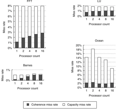
Figure I.8 shows the data miss rates for our four applications, as we increase the number of processors from 1 to 16, while keeping the problem size constant.

As we increase the number of processors, the total amount of cache increases, usually causing the capacity misses to drop. In contrast, increasing the processor count usually causes the amount of communication to increase, in turn causing the coherence misses to rise. The magnitude of these two effects differs by application.

In FFT, the capacity miss rate drops (from nearly 7% to just over 5%) but the coherence miss rate increases (from about 1% to about 2.7%), leading to a constant overall miss rate. Ocean shows a combination of effects, including some that relate to the partitioning of the grid and how grid boundaries map to cache blocks. For a typical 2D grid code the communication-generated misses are proportional to the boundary of each partition of the grid, while the capacity misses are proportional to the area of the grid. Therefore, increasing the total amount of cache while keeping the total problem size fixed will have a more significant effect on the capacity miss rate, at least until each subgrid fits within an individual processor’s cache. The significant jump in miss rate between one and two processors occurs because of conflicts that arise from the way in which the multiple grids are mapped to the caches. This conflict is present for direct-mapped and two-way set associative caches, but fades at higher associativities. Such conflicts are not unusual in array-based applications, especially when there are multiple grids in use at once. In Barnes and LU, the increase in processor count has little effect on the miss rate, sometimes causing a slight increase and sometimes causing a slight decrease.

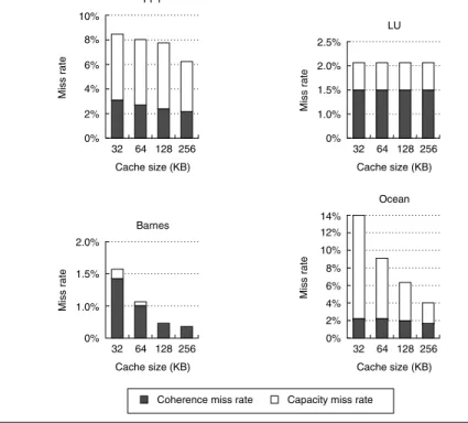
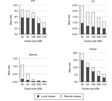
Increasing the cache size usually has a beneficial effect on performance, since it reduces the frequency of costly cache misses. Figure I.9 illustrates the change in miss rate as cache size is increased for 16 processors, showing the portion of the miss rate due to coherence misses and to uniprocessor capacity misses. Two effects can lead to a miss rate that does not decrease—at least not as quickly as we might expect—as cache size increases: inherent communication and plateaus

(24)

I-23

Figure I.8 Data miss rates can vary in nonobvious ways as the processor count is increased from 1 to 16. The miss rates include both coherence and capacity miss rates. The compulsory misses in these benchmarks are all very small and are included in the capacity misses. Most of the misses in these applications are generated by accesses to data that are potentially shared, although in the applications with larger miss rates (FFT and Ocean), it is the capacity misses rather than the coherence misses that comprise the majority of the miss rate. Data are potentially shared if they are allocated in a portion of the address space used for shared data. In all except Ocean, the potentially shared data are heavily shared, while in Ocean only the boundaries of the subgrids are actually shared, although the entire grid is treated as a potentially shared data object. Of course, since the boundaries change as we increase the processor count (for a fixed-size problem), different amounts of the grid become shared.

The anomalous increase in capacity miss rate for Ocean in moving from 1 to 2 processors arises because of conflict misses in accessing the subgrids. In all cases except Ocean, the fraction of the cache misses caused by coherence transactions rises when a fixed-size problem is run on an increasing number of processors. In Ocean, the coherence misses initially fall as we add processors due to a large number of misses that are write ownership misses to data that are potentially, but not actually, shared.

As the subgrids begin to fit in the aggregate cache (around 16 processors), this effect lessens. The single-processor numbers include write upgrade misses, which occur in this protocol even if the data are not actually shared, since they are in the shared state. For all these runs, the cache size is 64 KB, two-way set associative, with 32-byte blocks. Notice that the scale on the y-axis for each benchmark is different, so that the behavior of the individual benchmarks can be seen clearly.

Miss rate

0%

3%

2%

1%

1 2 4

Processor count FFT

8 16 8%

4%

7%

6%

5%

Miss rate

0%

6%

4%

2%

1 2 4

Processor count Ocean

8 16 16%

18%

20%

8%

14%

12%

10%

Miss rate 0%

1%

1 2 4

Processor count LU

8 16 2%

Miss rate 0%

1 2 4

Processor count Barnes

8 16 1%

Coherence miss rate Capacity miss rate

(25)

in the miss rate. Inherent communication leads to a certain frequency of coherence misses that are not significantly affected by increasing cache size. Thus, if the cache size is increased while maintaining a fixed problem size, the coherence miss rate eventually limits the decrease in cache miss rate. This effect is most obvious in Barnes, where the coherence miss rate essentially becomes the entire miss rate.

A less important effect is a temporary plateau in the capacity miss rate that arises when the application has some fraction of its data present in cache but some significant portion of the dataset does not fit in the cache or in caches that are slightly bigger. In LU, a very small cache (about 4 KB) can capture the pair of 16 × 16 blocks used in the inner loop; beyond that, the next big improvement in capacity miss rate occurs when both matrices fit in the caches, which occurs when the total cache size is between 4 MB and 8 MB. This effect, sometimes called a working set effect, is partly at work between 32 KB and 128 KB for FFT, where the capacity miss rate drops only 0.3%. Beyond that cache size, a faster decrease in the capacity miss rate is seen, as a major data structure begins to reside in the cache. These plateaus are common in programs that deal with large arrays in a structured fashion.

Figure I.9 The miss rate usually drops as the cache size is increased, although coher- ence misses dampen the effect. The block size is 32 bytes and the cache is two-way set associative. The processor count is fixed at 16 processors. Observe that the scale for each graph is different.

Miss rate

0%

4%

2%

32 64 128 Cache size (KB)

FFT

256 10%

6%

8%

Miss rate

0%

1.5%

1.0%

LU

256 2.5%

2.0%

Miss rate

0%

6%

2%

4%

Ocean

256 14%

10%

8%

12%

Miss rate

0%

1.0%

Barnes

256 2.0%

1.5%

(26)

I-25

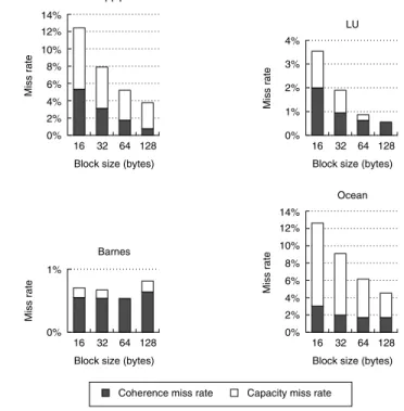
Increasing the block size is another way to change the miss rate in a cache. In uniprocessors, larger block sizes are often optimal with larger caches. In multiprocessors, two new effects come into play: a reduction in spatial locality for shared data and a potential increase in miss rate due to false sharing. Several studies have shown that shared data have lower spatial locality than unshared data. Poorer locality means that, for shared data, fetching larger blocks is less effective than in a uniprocessor because the probability is higher that the block will be replaced before all its contents are referenced. Likewise, increasing the basic size also increases the potential frequency of false sharing, increasing the miss rate.

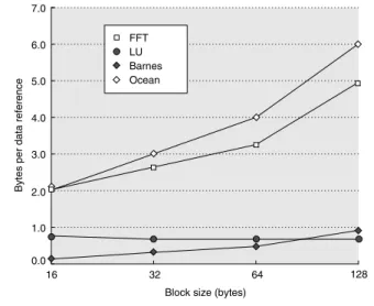
Figure I.10 shows the miss rates as the cache block size is increased for a 16-processor run with a 64 KB cache. The most interesting behavior is in Barnes, where the miss rate initially declines and then rises due to an increase in the number of coherence misses, which probably occurs because of false sharing. In the other benchmarks, increasing the block size decreases the overall miss rate. In Ocean and LU, the block size increase affects both the coherence and capacity miss rates about equally. In FFT, the coherence miss rate is actually decreased at a faster rate than the capacity miss rate. This reduction occurs because the communication in FFT is structured to be very efficient. In less optimized programs,

Figure I.10 The data miss rate drops as the cache block size is increased. All these results are for a 16-processor run with a 64 KB cache and two-way set associativity.

Once again we use different scales for each benchmark.

Miss rate

0%

6%

4%

2%

16 32 64 Block size (bytes)

FFT

128 14%

10%

8%

12%