SOM: Dynamic Push-Pull Channel Allocation Framework

(1)

SOM: Dynamic Push-Pull Channel Allocation Framework for Mobile Data Broadcasting

Jiun-Long Huang, Wen-Chih Peng

^†

and Ming-Syan Chen, Fellow, IEEE Department of Electrical Engineering

National Taiwan University Taipei, Taiwan, ROC

†

Department of Computer Science and Information Engineering Nation Chiao-Tung University

Hsinchu, Hsinchu, ROC

E-mail: [email protected], [email protected], [email protected]

Abstract

In a mobile computing environment, the combined use of broadcast and on-demand channels can utilize the bandwidth effectively for data dissemination. We explore in this paper the problem of dynamic data and channel allocation with the number of communication channels and the number of data items given. We first derive the analytical models of the average access time when the data items are requested through the broadcast and on-demand channels. Then, we transform this problem into a guided search problem. In light of the theoretical properties derived, we devise algorithm SOM to obtain the optimal allocation of data and channels. Algorithm SOM is a composite algorithm which will cooperate with (1) a search strategy and (2) a broadcast program generation algorithm. According to the analytical mode, we devise scheme BIS-Incremental on the basis of algorithm SOM which is able to obtain solutions of high quality efficiently by employing binary interpolation search. In essence, scheme BIS-Incremental is guided to explore the search space with higher likelihood to be the optimal first, thereby leading to an efficient and effective search.

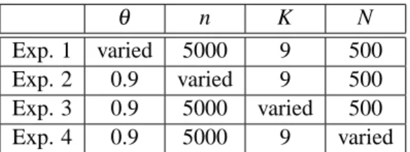
It is shown by our simulation results that the solution obtained by scheme BIS-Incremental is of very high quality and is in fact very close to the optimal one. Sensitivity study on several parameters, including the number of data items and the number of communication channels, is conducted.

The experimental results shows that scheme BIS-Incremental is of very good scalability which is particularly important for its practical use in a mobile computing environment.

Key words: Data dissemination, dynamic data and channel allocation, mobile computing

(2)

1 Introduction

In a mobile computing environment, a mobile user with a power-limited mobile computer can access various information via wireless communication. Applications such as stock activities, traffic reports and weather forecast have become increasingly popular in recent years [29]. It is noted that mobile computers use small batteries for their operations without directly connecting to any power source, and the bandwidth of wireless communication is in general limited. As a result, an important design issue in a mobile system is to conserve the energy and communication bandwidth of a mobile unit while allowing mobile users of the ability to access information from anywhere at anytime [24].

A data delivery architecture in which a server continuously and repeatedly broadcasts data to a client community through a single broadcast channel was proposed in [1] in order to conserve the energy and communication bandwidth of a mobile computing system. In a push-based information system, a server generates a broadcast program to broadcast data to mobile users. This broadcast channel is also referred to as a broadcast disk from which mobile users can retrieve data [1][7]. The mobile users need to wait for the data of interest to appear on the broadcast channel. The access time is defined as the time elapsed from the moment a user issues a data request to the point that the requested data item is read [15]. One objective of designing proper data allocation in the broadcast disks is to reduce the average access time of data items. The research issues have attracted a considerable amount of attention, including on-demand broadcast [3][4][5][6], data indexing [9][14][15][17][30][33] and client cache management [4][27][31]. In addition, a significant amount of research effort has been elaborated on developing the index mechanisms [16][20][25] and data allocation algorithms [22][23][28][34][35] in multiple broadcast channels. In addition, the bandwidth allocation for multi-cell environments with frequency reuse and inference considered was studied in [32].

In addition to being operated in broadcast mode, channels can be operated in on-demand mode (i.e., unicast mode) in which a client explicitly sends data requests to retrieve the data items of interest [18][19]. The major advantage of data broadcast is its scalability since the performance of the system does not depend on the number of clients listening to the broadcast channels. However, the performance degrades as the number of data items being broadcast increases. It has been shown that the

(3)

combined use of the broadcast and on-demand channels can utilize bandwidth more efficiently for data dissemination [18][19]. Hence, the problem of dynamic data and channel allocation is to dynamically partition a given total number of communication channels into broadcasting ones and on-demand ones and to dynamically allocate each data item on broadcast or on-demand channel according to the system workload.

Prior studies of data and channel allocation can be classified into the following three categories: (1) pure on-demand, (2) pure broadcast and (3) dynamic data and channel allocation. The pure on-demand algorithms are used in traditional client/server architectures. All channels are operated in on-demand mode, and all data items are allocated in the on-demand channels. Clients explicitly send data requests to the server to obtain the desired data items. This method is desirable when the number of requests is small and when energy saving is not an issue for the mobile devices. In pure broadcast, all channels are allocated in broadcast mode [1][12][22][35], and all data items are broadcast repeatedly in broadcast channels. This method is useful when the access frequencies of data items are highly skewed (i.e., a small number of data items are of interest to a large group of users).

Dynamic data and channel allocation algorithms are proposed to combine the respective merits of on-demand and broadcast modes and to adapt the change of system parameters including the data access frequencies and the number of users in the system [18][19][26]. In dynamic data and channel allocation, the system dynamically allocates broadcast and on-demand channels in accordance with data requests to achieve optimal data access performance. When the load is heavy, the broadcast channels may significantly relieve the load on on-demand channels by broadcasting frequently accessed data items. When the load is light, on-demand channels can take over to provide instantaneous access to data items.

In this paper, we study the problem of dynamic data and channel allocation. Consider the illustrative example shown in Figure 1. Assume that the data items R_i, 1 ≤ i ≤ 15, are of the same size and are sorted by their access frequencies. The number of channels in this example is assumed to be four. In the beginning, two channels are assigned as broadcast channels and the other two are on-demand ones.

Five data items are put in broadcast channels and the broadcast program is shown in Figure 1a. When

(4)

R₁ R₂

R₃ R₄ R₅

On-demand Channel On-demand Channel Broadcast

Channels

R₆-R₁₅

(a)

R₁ R₂

R₃ R₄ R₅

On-demand Channel On-demand Channel Broadcast

Channels

R₇-R₁₅

R₆

(b)

R₁ R₂

R₃ R₄ R₅

On-demand Channel Broadcast

Channels

R₁₀-R₁₅

R₆ R₇ R₈ R₉

(c) Figure 1: An example scenario of dynamic data and channel allocation

the data request rate increases, R₆ is moved from the on-demand channel to the broadcast channel.¹ This will reduce the data request rate to on-demand channels and the expected waiting time in on- demand channels is hence reduced. The broadcast program is then rescheduled and the new broadcast program is shown in Figure 1b. If the data request rate keeps increasing, as shown in Figure 1c, one channel is re-assigned to be a broadcast one and three data items (R₇, R₈and R₉) are moved from on- demand channels to broadcast channels. As the partition of broadcast and on-demand channels varies, the number of data items in those channels changes accordingly, showing the dynamic characteristics of this data and channel allocation problem.

We mention in passing that the authors of [26] provide an adaptive algorithm to allocate data items on broadcast and on-demand channels. However, they assume a fixed ratio of the on-demand bandwidth to the broadcast bandwidth. The work in [19] is designed to shuffle the loads among broadcast and on-demand channels to keep the load of on-demand channels in a predetermined region. In [18], the average access time of data items is formulated, and the optimal channel allocation is obtained ac- cording to the derived theoretical results. Both works [18] and [19] employed flat broadcast programs.

A broadcast program is said flat if all data items appear with the same frequencies in the broadcast program. On the other hand, a broadcast program is said hierarchical if data items of high access fre- quencies are broadcast more frequently than or equal to those of low access frequencies in the broadcast program. It has been shown that hierarchical broadcast programs usually outperform flat broadcast programs [22][23]. Hence, algorithms proposed by [18] and [19] may not fully utilize network bandwidth.

In view of this, we employ hierarchical broadcast programs in this paper in order to fully utilize the

1The criterion for data movement will be given in Section 4 later.

(5)

broadcast channels. This feature distinguishes this paper from others.

Explicitly, we explore in this paper the problem of dynamic data and channel allocation with the number of communication channels and the number of data items given. Gathering the access frequencies of data items is another research issue, since clients do not explicitly send data requests when the data items of interest are put in broadcast channels. Research works [13][36] in gathering or estimat- ing the data access frequencies in broadcast channels can complement our work. Different from the prior studies [18][19], hierarchical broadcast programs are employed in our study. In this paper, we first describe the analytical models of broadcast and on-demand channels and transform the problem of dynamic data and channel allocation into a guided search problem. In light of the theoretical properties derived, we devise five pruning properties which are able to effectively reduce the search space by removing the infeasible solutions from the search space. We then devise algorithm SOM (standing for SOlution Mapping) to obtain the optimal allocation of data and channels. Algorithm SOM is a compos- ite algorithm which will cooperate with (1) a search strategy and (2) a broadcast program generation algorithm. According to the analytical models, we devise a search strategy called BIS (standing for Binary Interpolation Search) which is able to dynamically partition the data items and channels into broadcast and on-demand ones in accordance with the incoming requests. Then, based on algorithm SOM, we devise scheme BIS-Incremental to obtain solutions of high quality efficiently by employing BIS as the search strategy and VF^K(standing for Variant-Fanout with the constraint K) as the broadcast program generation algorithm². In essence, scheme BIS-Incremental is guided to explore the search space with higher likelihood to be the optimal first, thereby leading to an efficient and effective search.

In addition, scheme BIS-Incremental takes advantage of the incremental property of VF^Kwhich greatly reduces the execution time. It is shown by our simulation results that the solutions obtained by scheme BIS-Incremental are of very high quality and are in fact very close to the optimal ones. Sensitivity study on several parameters, including the number of data items and the number of communication channels, is conducted. Moreover, scheme BIS-Incremental is of very good scalability which is particularly important for its practical use in a mobile computing environment.

The rest of this paper is organized as follows. A description of the related work is given in Section 2.

2An introduction of algorithm VF^Kwill be given in Section 3.1.

(6)

In addition, the problem of dynamic data and channel allocation is also formulated. Then the analytical models of broadcast, on-demand channels and the overall system are given in Section 3. In Section 4, we transform the problem of dynamic data and channel allocation into a search problem and develop an efficient algorithm to address this problem based on the derived analytical models. The performance evaluation of the proposed algorithm is presented in Section 5. Finally, this paper concludes with Section 6.

2 Preliminaries

2.1 Related Work

In [2], the architecture consisting of a single uplink channel and a broadcast channel is considered. A portion of time slots on the broadcast channel is allocated to transmit the data items which are explicitly requested by users via the uplink channel. These time slots are said to be in on-demand mode. On the other hand, the remaining time slots are used to transmit all data items according to a hierarchical broadcast program generated by the broadcast disk technique [1]. These time slots are said to be in broadcast mode. In [2], the ratio of the time slots in broadcast mode to those in on-demand mode is fixed, and the broadcast program is static. As a consequence, the scheme proposed in [1] cannot adapt to the change of system workload.

The authors in [26] consider the environment with a broadcast channel, a downlink on-demand channel and an uplink channel. The on-demand channel is dedicated to transmit the data items which are explicitly requested by users via the uplink channel. Flat broadcast programs are employed and only the data items whose request rates are high enough will be allocated on the broadcast channel. The authors propose an algorithm to estimate the popularity of all data items and to dynamically determine the set of data items on the broadcast channel according to the system workload.

In [10], the information system consists of a broadcast channel and an uplink channel. The authors propose an algorithm to prioritize all data items according to the received data requests and the broadcast rates of these data items. Then, the algorithm will allocate the data items with highest priorities on the broadcast channel. The flat broadcast programs are used and (1, m) indexing technique [15]

(7)

is employed to construct data indices. The authors also propose several energy efficient data access protocols to minimize the power consumption on data access.

In [19], the authors consider the environments with a single broadcast channel and multiple on- demand channels. The broadcast programs are assumed to be flat. The load of the on-demand channels are first divided into several regions. Then, the authors propose a data allocation algorithm to keep the load of the on-demand channels in a predetermined sub-optimal region by dynamically allocating some data items to the broadcast channel. In addition, the proposed algorithm is able to adaptively adjust the data allocation according to the system workload.

The authors in [18] consider the environments with multiple broadcast and on-demand channels.

The broadcast programs on the broadcast channels are assumed to be flat. The authors first model the on-demand channels as an M/M/c queue. Then, the formulae of the average access time of the broadcast and on-demand channels are derived. With these analytical results, the authors propose a data and channel allocation algorithm to determine (1) the numbers of channels which are operated in broadcast and on-demand modes and (2) the data items which are allocated in the broadcast and on- demand channels according to the system workload. However, since the proposed algorithm does not employ hierarchical broadcast programs, the network bandwidth may not be fully utilized. The problem we address is similar to that considered in [18], but different from the latter in that, we also consider the generation of hierarchical broadcast programs to attain a higher network bandwidth utilization.

2.2 System Description and Problem Formulation

Denote the total number of data items as n, and data items as R_i, 1 ≤ i ≤ n. Naturally, the n_B frequently accessed data items are placed in broadcast channels and the other n_O= n − n_B data items are in on- demand channels. Let K = K_B+ K_O represent the total number of channels where K_B and K_Oare the numbers of broadcast and on-demand channels, respectively. The problem of generating broadcast programs for K_B broadcast channels can be viewed as the following discrete minimization problem:

Given a set of n_B data items with their access probabilities, partition them into K_B parts so that the average access time of all data items is minimized [12][22][23][35]. Note that once K_B is decided, K_O follows.

(8)

R₁ R₂ R₃

R_n

Data and channel allocation scheme

Channel 1 Channel 2 Channel K

Channel 1 Channel 2 Channel K_B

Channel K_B+1 Channel K_B+2 Channel K

R₁

R₁ R₁

R₂ R₃

R₁

R₃ R₂

Broadcast

On-demand Broadcast

Program Access

Frequencies

Notebook PDA Mobile Device

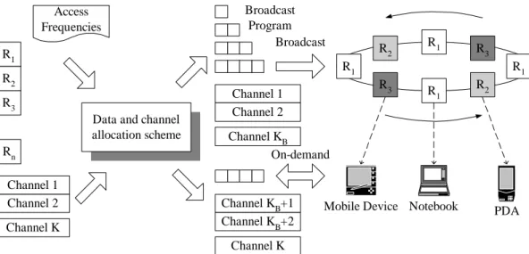
Figure 2: The architecture of a data dissemination system

Figure 2 shows the architecture of a data dissemination system. We assume that each data item is the same size and read-only [18][19]. After being powered on, without knowing the placement of the requested data item, a mobile device has to send a data item request via on-demand channels. If the requested data item is placed in an on-demand channel, the server will reply the data item directly.

If the data item is in a broadcast channel, the server replies the broadcast information containing the channel frequencies, the data identifiers, the data index information, and other auxiliary information [18]. After receiving the broadcast information, the mobile device will store the broadcast information in the local storage, listen to the broadcast channel and wait for the requested data item.

If a mobile device already has the broadcast information in its local storage, for each user request, the device will check whether the requested data item is placed in broadcast channels. If yes, the device will tune to the channel where the required data item is placed and wait for the appearance of the requested data item. Otherwise, the device will explicitly send a data request to the server via an on-demand channel and the server will return the requested data item on the on-demand channel.

With the above model, the problem of dynamic data and channel allocation we consider in this paper is formulated as follows:

Problem of dynamic data and channel allocation: Given K channels, n data items and their access frequencies, we shall do the following tasks to minimize the average access time of all data items.

1. Determine the numbers of broadcast and on-demand channels (i.e., K_B and K_O), where K =

(9)

K_B+ K_O.

2. Determine the numbers of data items allocated to broadcast and on-demand channels (i.e., n_Band n_O), where n = nB+ n_O.

3. Construct a hierarchical broadcast program in the K_B broadcast channels with the n_B most frequently accessed data items.

3 Analytical Models

The analytical models of the broadcast and on-demand channels are given in Section 3.1 and Sec- tion 3.2, respectively. In accordance with these analytical models, the overall average access time is formulated in Section 3.3. For better readability, Table 1 lists the symbols used in this paper.

3.1 Broadcast Channels

Since there is more than one data broadcast program for given K_B and n_B, we use W_B(K_B, n_B) to repre- sent the minimal average access time of the data items allocated in broadcast channels. Let C(K₁, n₁) be a configuration where K_B = K₁ and n_B = n₁. The optimal broadcast program can be obtained by executing one broadcast program generation algorithm.

Without considering the use of on-demand channels, the work in [22] explored the problem of generating broadcast programs with the number broadcast channels (i.e., K_B) given. Specifically, the problem of generating broadcast programs for K_B broadcast channels was transformed into a partition problem to partition the data items into K_B partitions. The data items within the same partition are periodically broadcast in the same channel. Two algorithms, OPT and VF^K, were devised in [22]

to generate hierarchical broadcast programs for multiple broadcast channels. Algorithm OPT is an A^∗-like algorithm which is able to generate the optimal broadcast program. However, OPT is quiet time-consuming. On the other hand, VF^K is a greedy, heuristic algorithm which is able to efficiently obtain broadcast programs which are shown to be very close to the optimal ones. Since the details of OPT and VF^K are beyond the scope of this paper, interested readers are referred to [22] for the details

(10)

Description Symbol

Number of channels K

Number of broadcast channels K_B

Number of on-demand channels K_O

Number of data items n

Number of data items in broadcast channels nB

Number of data items in on-demand channels nO

The j-th data item Rj

The access frequency of data item Rj Pr(Rj)

The size of each data item s

The size of each data request r

The channel bandwidth b

The data request rate λ

The average service time for each on-demand channel _µ¹ Table 1: Description of symbols

of OPT and VF^K. To facilitate the design of scheme BIS-Incremental, an overview of VF^K is given as follows.

Basically, VF^K is a partition-based algorithm which divides all data items into K partitions where K is the number of broadcast channels, and allocates all data items into K broadcast channels according to the resultant partitions. Initially, all data items, R₁, R₂, · · · R_n, are reordered according to their access frequencies in descendent order, and are placed in one partition. The average access time of a partition is defined as the average access time of the case that the data items of the partition are broadcast periodically in one broadcast channel. Then, the average access time of a broadcast program on multiple channels is the summation of the average access times of all partitions. In each cut, the partition with the largest average access time, say {R_p, R_p+1, · · · , R_q}, is selected, and the best cut point of the selected partition, say c, which best reduces the average access time of the broadcast program is determined.

Then, the selected partition is cut into two partitions, {R_p, R_p+1, · · · , R_c} and {R_c+1, R_c+2, · · · , R_q}.

For K_B broadcast channels, K_B− 1 cuts are sequentially performed to partition the data items into K_B partitions. Finally, the resultant broadcast program is obtained by periodically broadcasting all data items within the same partition in one broadcast channel.

Then, we have the incremental property of VF^K as follows. For interest of space, the proof of all properties and lemmas is given in Appendix.

(11)

Lemma 1 (Incremental Property): The execution of VF^K on configuration C(K₁, n₁) will generate K₁data broadcast programs of C(K_b, n₁), 1 ≤ K_b≤ K₁.

Lemma 1 means that the execution of VF^K on configuration C(K₁, n₁) will generate K₁broadcast programs which are the same as the results produced by VF^K for configurations C(K_B, n₁) where K_B=1, 2, 3, · · ·, K₁.

3.2 On-demand Channels

Let WO(KO, nO) denote the average access time of the data items placed in on-demand channels. Let P_Oⁿ(n_O) be the probability that the requested data item is in on-demand channels when there are n_Odata items placed in on-demand channels. We assume that the arrival process of user requests is a Poisson process with the arrival rateλ. It follows that the arrival process of requests received by on-demand channels is also a Poisson process with arrival rateλO= P_Oⁿ(n_O)λ. Same as in [18], we assume that the queueing buffer is infinite. Thus, the on-demand channels are modeled as an M/M/c queueing system [11] with the arrival rate λO, the service rate µ and the channel number c. The average service time is _µ¹. Let the sizes of data items and data requests be s and r, respectively. Hence, similar to [18], the average service time of on-demand channels can be formulated as:

µ⁼ ^b s + r.

Omitting the equation manipulation which can be found in [11], the average access time of the on- demand channels (i.e., the M/M/c queueing system where c = K_O) whenρ ^{< 1 is}

Average access time = 1 µ ⁺

µ r^c

c!(cµ^{)(1 −}ρ⁾²

¶

p₀, where (1)

ρ⁼ λO

cµ^{, r =} λO

µ ^{, and p}⁰⁼ Ãc−1

n=0

∑

rⁿ

n!+ r^c c!(1 −ρ⁾

!₋₁ .

(12)

No. of Data Items in Broadcast Channels (n_B)

Average Access Time

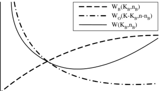
W_B(K_B,n_B) W_O(K-K_B,n-n_B) W(K_B,n_B)

Figure 3: Trade-off for dynamic data dissemination

3.3 Overall Average Access Time

The probability that a user requests a data item placed in the broadcast channels is P_Bⁿ(n_B) =∑ⁿ_i=1^B Pr(R_i).

On the other hand, the probability that a user requests a data item placed in the on-demand channels is P_Oⁿ(n_O) =∑ⁿ_i=n−n_O₊₁Pr(Ri) = 1 −∑ⁿ_i=1^B Pr(Ri) = 1 − P_Bⁿ(nB). Then, the minimal average access time of a data dissemination system can then be formulated as follows:

W_optimal(K, n) = min

0≤KB≤K,0≤nB≤n{W (KB, nB)}, where (2)

W (KB, nB) = P_Bⁿ(nB) ×WB(KB, nB) + (P_Oⁿ(n_O)) ×W_O(K_O, n_O)

= P_Bⁿ(n_B) ×W_B(K_B, n_B) + (1 − P_Bⁿ(n_B)) ×W_O(K − K_B, n − n_B).

With K_Bpredetermined, the relationship among W (K_B, n_B), W_B(K_B, n_B) and W_O(K − K_B, n − n_B) is plotted in Figure 3. Note that W_O(K −K_B, n−n_B) increases exponentially when n_Oincreases (i.e., when nB decreases). It is evident that with too few data items in broadcast channels, the volume of requests at the servers may increase beyond their capacity, thereby making the service practically infeasible. On the other hand, the change of the average access time for the broadcast data items is smoother than that for the on-demand data items since the average access time of the broadcast data items only depends on the number of data items allocated to broadcast channels. In this study, the dynamic data and channel allocation algorithm designed will determine the proper values of K_B and n_B with the objective of

(13)

minimizing the average access time of all data items.

4 SOM: Solution Mapping on Broadcast and On-demand Chan- nels

In this section, we design algorithm SOM based on the analytical results in Section 3 to address the problem of dynamic data and channel allocation. In Section 4.1, we transform the problem of dynamic data and channel allocation into a search problem and give an overview of algorithm SOM. In Section 4.2, several properties to prune the infeasible solutions from the search space are given. Then, an efficient search strategy based on binary interpolation search, referred to as BIS, is devised in Section 4.3.

Based on algorithm SOM, scheme BIS-Incremental, which is able to obtain nearly-optimal solutions by employing BIS and the incremental properties of VF^K, is then proposed. The complexity analysis of scheme BIS-Incremental is given in Section 4.4. Finally, an illustrative example is given in Section 4.5.

4.1 Problem Transformation and Overview of SOM

Given K and n, for each configuration C(K_B, n_B), W_B(K_B, n_B) can be obtained by executing a broadcast program generation algorithm, and W_O(K − K_B, n − n_B) can be calculated by the analytical model of the on-demand channels. As a result, the problem can be transformed into a search problem: to find the configuration with the minimal average access time by searching all given configurations C(K_B, n_B), where 0 ≤ K_B≤ K and 0 ≤ n_B≤ n.

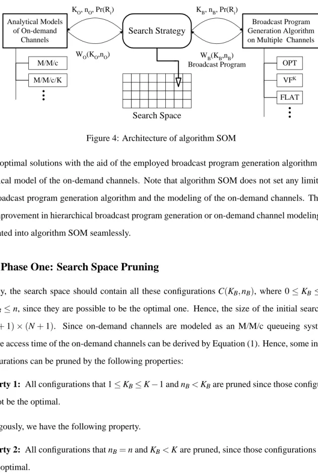
We design in this section algorithm SOM to address the problem of dynamic data and channel allocation. In essence, algorithm SOM is a composite and generic algorithm which is composed of a search strategy and a broadcast program generation algorithm. Algorithm SOM consists of two major phases: the search space pruning phase and the solution searching phase. Figure 4 shows the architecture of algorithm SOM. In search space pruning phase, some infeasible configurations are removed from the search space. Then, in solution searching phase, a search strategy is used to guide the search

(14)

Search Strategy

Broadcast Program Generation Algorithm on Multiple Channels K_B, n_B, Pr(R_i)

W_B(K_B,n_B) Broadcast Program

Search Space

OPT VF^K FLAT Analytical Models

of On-demand Channels

K_O, n_O, Pr(R_i)

W_O(K_O,n_O) M/M/c

M/M/c/K

Figure 4: Architecture of algorithm SOM

of the optimal solutions with the aid of the employed broadcast program generation algorithm and the analytical model of the on-demand channels. Note that algorithm SOM does not set any limitation in the broadcast program generation algorithm and the modeling of the on-demand channels. Therefore, any improvement in hierarchical broadcast program generation or on-demand channel modeling can be integrated into algorithm SOM seamlessly.

4.2 Phase One: Search Space Pruning

Initially, the search space should contain all these configurations C(K_B, n_B), where 0 ≤ K_B ≤ K and 0 ≤ n_B≤ n, since they are possible to be the optimal one. Hence, the size of the initial search space is (K + 1) × (N + 1). Since on-demand channels are modeled as an M/M/c queueing system, the average access time of the on-demand channels can be derived by Equation (1). Hence, some infeasible configurations can be pruned by the following properties:

Property 1: All configurations that 1 ≤ K_B≤ K − 1 and n_B< K_Bare pruned since those configurations will not be the optimal.

Analogously, we have the following property.

Property 2: All configurations that n_B= n and K_B< K are pruned, since those configurations will not be the optimal.

Omitting straightforward proofs, we also have the following three properties.

(15)

n-1 K-1

2 1 0 K

0 1 2 3 4 5 n

1 1 1,4

1

3 1,4

2 2 2,3 3 4

1 1 1 1 1 1 2

Number of Data Items within Broadcast Channels (n_B) Number of Broadcast Channels (K B)

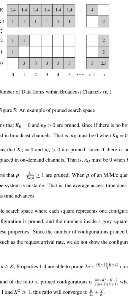
Figure 5: An example of pruned search space

Property 3: All configurations that K_B= 0 and n_B> 0 are pruned, since if there is no broadcast chan- nel, no data item can be placed in broadcast channels. That is, n_Bmust be 0 when K_B= 0.

Property 4: All configurations that K_O = 0 and n_O> 0 are pruned, since if there is no on-demand channel, no data item can be placed in on-demand channels. That is, n_Omust be 0 when K_O= 0.

Property 5: All configurations thatρ ⁼ _K^λ_O^O_µ ≥ 1 are pruned. When ρ of an M/M/c queueing system is larger than or equal to 1, the system is unstable. That is, the average access time does not converge and will increase drastically as time advances.

Figure 5 shows an example search space where each square represents one configuration. A grey square indicates that this configuration is pruned, and the numbers inside a grey square indicate this configuration is pruned by these properties. Since the number of configurations pruned by Property 5 depends on other parameters such as the request arrival rate, we do not show the configurations pruned by Property 5 in Figure 5.

Lemma 2: When K ≥ 1 and n ≥ K, Properties 1-4 are able to prune 2n +^(K−1)(K+2)₂ configurations.

Lemma 3: (1) The lower bound of the ratio of pruned configurations is 2(n+1)(K+1)^4n+K²^+K−2 when K ≥ 1 and n ≥ K. (2) When n ≥ K, n À 1 and K²À 1, this ratio will converge to _2n^K +_K².

(16)

In phase one, after building the initial search space, algorithm SOM will prune the infeasible configurations according to Properties 1-5. Then, algorithm SOM will search the pruned search space for the optimal configuration in phase two.

4.3 Phase Two: Solution Searching

4.3.1 Design of Search Strategy BIS

In phase two of algorithm SOM, a search strategy is employed to search the pruned search space for the optimal configuration. It is obvious that the optimal configuration can be obtained by exhaustive search. However, it is not scalable when the size of the pruned search space is large.

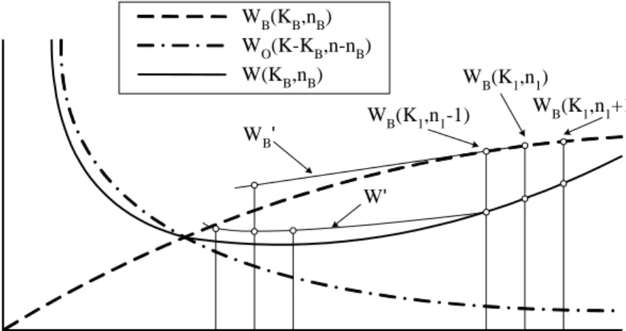
To achieve high scalability, we devise an efficient search strategy, referred to as BIS, based on the analytical models. BIS is a greedy algorithm to find the sub-optimal solution of the search space. In essence, BIS is guided to explore the search space with higher likelihood to be the optimal first. A configuration C(K1, n1) is said to be “local optimal when KB= K1” if W (K1, n1− 1) ≥ W (K1, n1) and W (K₁, n₁+1) ≥ W (K₁, n₁). To facilitate the design of BIS, we employ the function LocalOptimalCheck to determine whether the input configuration is local optimal. LocalOptimalCheck(K₁, n₁) returns LOCALOPTIMAL to notify BIS that the input configuration C(K1, n1) is the local optimal when KB= K1. Otherwise, it returns MINUS and PLUS to show that W (K₁, n₁− 1) < W (K₁, n₁) and W (K₁, n₁+ 1) <

W (K₁, n₁), respectively. The algorithmic form of LocalOptimalCheck is as follows.

Function LocalOptimalCheck(K_B, n_B)

1: Calculate(K_B,n_B− 1)

2: Calculate(K_B,n_B+ 1)

3: if (W (K_B, n_B− 1) < W (K_B, n_B)) then

4: return MINUS

5: else if (W (K_B, n_B+ 1) < W (K_B, n_B)) then

6: return PLUS

7: else /* W (K_B, n_B− 1) ≥ W (K_B, n_B) and W (K_B, n_B+ 1) ≥ W (K_B, n_B) */

8: return LOCALOPTIMAL

9: end if

Procedure Calculate(K_B,n_B)

1: Calculate and store WB(KB, nB) and the corresponding broadcast program by employed broadcast program generation algorithm if they had not been calculated

2: Calculate and store W_O(K − KB, n − nB) by Equation (1) if it had not been calculated

(17)

Number of Broadcast Items (n_B)

Average Access Time

W_B(K₁,n₁-1)

W_B(K₁,n₁)

W_B'

W'

n₁-1 n₁ n₂-1 n₂ n₂+1

W_B(K₁,n₁+1) W_B(K_B,n_B)

W_O(K-K_B,n-n_B) W(K_B,n_B)

n₁+1

Figure 6: Execution scenario of function LocalOptimalPrediction

3: Calculate and store W (K_B, n_B) by Equation (2) if it had not been calculated

Note that each invocation of LocalOptimalCheck will cause at least one execution of the broadcast program generation algorithm. That is costly. Therefore, we design function LocalOptimalPrediction to predict the position of the local optimal solution to reduce the total execution time by reducing the number of invocations of LocalOptimalCheck.

To facilitate the design of function LocalOptimalPrediction, we first design a method to calcu- late the approximations of W_B(K_B, n_B) and W (K_B, n_B). Denote the approximations of W_B(K_B, n_B) and W (K_B, n_B) as W_B⁰(K_B, n_B) and W⁰(K_B, n_B), respectively. Figure 6 shows the proposed approximation method which calculates W_B⁰(KB, nB) and W⁰(KB, nB) by extrapolation. As shown in Figure 6, the value of W_B⁰(K₁, n₂), for each n₂, can be obtained by the extrapolation of W_B(K₁, n₁) and W_B(K₁, n₁− 1).

Then, we have the following equation:

W_B⁰(K₁, n₂)

n₂− n₁ =W_B(K₁, n₁+α^{) −W}B(K₁, n₁)

α ^{, where}

α ⁼





1 : if LocalOptimalCheck(K₁, n₁) returns PLUS, -1 : if LocalOptimalCheck(K₁, n₁) returns MINUS.

(18)

By solving the above equation, we have W_B⁰(K₁, n₂) as:

W_B⁰(K₁, n₂) = 1

α ^{× (n}²^{− n}¹^{) × (W}^B^(K¹^{, n}¹⁺α^{) −W}B(K₁, n₁)).

Since W_O(K₁, n₂) can be obtained by Equation (1), with W_B⁰(K₁, n₂), W⁰(K₁, n₂) can be obtained by the following equation:

W⁰(K₁, n₂) = P_Bⁿ(n₂) ×W_B⁰(K₁, n₂) + (1 − P_Bⁿ(n₂)) ×W_O(K − K₁, n − n₂). (3)

LocalOptimalPrediction is employed to predict the position of the local optimal of the configura- tions with K_B= K₁ and n_Lower ≤ n_B ≤ n_{U pper}. First, LocalOptimalPrediction sets n₁= ^dn^Lower⁺ⁿ₂ ^{U pper}^e and checks whether W⁰(K₁, n₁− 1) ≥ W⁰(K₁, n₁) and W⁰(K₁, n₁+ 1) ≥ W⁰(K₁, n₁). That is to check whether W⁰(K1, n1) is local optimal. If so, LocalOptimalPrediction reports C(K1, n1) as the possible configuration of the local optimal solution. Otherwise, if W⁰(K₁, n₁− 1) < W⁰(K₁, n₁), LocalOptimal- Prediction is invoked recursively by setting n_{U pper}= n₁− 1. Similarly, if W⁰(K₁, n₁+ 1) < W⁰(K₁, n₁), LocalOptimalPrediction is invoked recursively by setting nLower = n1+ 1. The algorithmic form of function LocalOptimalPrediction is as follows.

Function LocalOptimalPrediction(K1, nLower, nU pper)

1: n1← ^dn^Lower⁺ⁿ₂ ^{U pper}^e

2: Calculate W⁰(K₁, n₁), W⁰(K₁, n₁− 1) and W⁰(K₁, n₁+ 1) by Equation 3

3: if (W⁰(K₁, n₁+ 1) < W⁰(K₁, n₁)) then

4: return LocalOptimalPrediction(K₁, n₁+ 1, n_{U pper})

5: else if (W⁰(K₁, n₁− 1) < W⁰(K₁, n₁)) then

6: return LocalOptimalPrediction(K₁, n_Lower, n₁− 1)

7: else /* W⁰(K₁, n₁) is local optimal */

8: return n₁

9: end if

We now design search strategy BIS using LocalOptimalCheck and LocalOptimalPrediction. After the search space is pruned, BIS checks these unpruned configurations iteratively. In each iteration, BIS picks one value (denoted as K₁) from the possible values of K_B, sets K_B= K₁ and considers the configurations with KB = K₁. Suppose that nMax and nMin are the maximum and minimum, respec- tively, of n_B among all unpruned configurations with K_B= K₁. BIS sets n₁= dⁿ^Max⁺ⁿ₂ ^Mine and checks

(19)

whether or not the configuration C(K₁, n₁) is the local optimal with K_B = K₁ by LocalOptimalCheck.

If LocalOptimalCheck returns LOCALOPTIMAL, BIS memorizes configuration C(K₁, n₁) as a candidate of the resultant configuration. Then, BIS steps into next iteration by picking another value of K₁. Otherwise, when LocalOptimalCheck returns PLUS or MINUS, LocalOptimalPrediction is invoked to predict the position of the local optimal with K_B = K₁. Suppose that LocalOptimalPrediction reports that C(K₁, n₂) has the high probability to be the local optimal when KB= K₁. LocalOptimalCheck is invoked again to check whether W (K₁, n₂) is the local optimal. In one iteration, BIS repeats the above procedure until the configuration predicted by LocalOptimalPrediction is indeed the local optimal (i.e., LocalOptimalCheck returns LOCALOPTIMAL). After picking all possible values of KB, BIS stops and returns the best solution among the candidates.

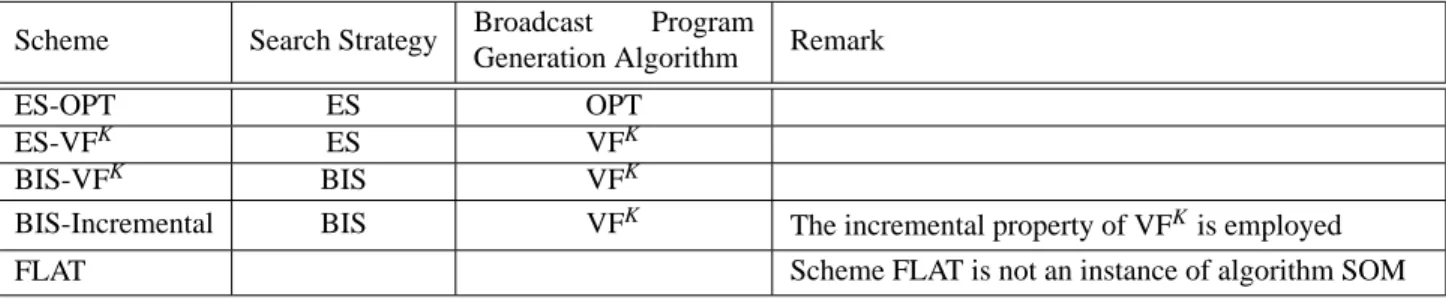
For better understanding of algorithm SOM and search strategy BIS, we design scheme BIS-Generic by employing BIS as the search strategy of algorithm SOM. Without being limited to any broadcast program generation algorithm, scheme BIS-Generic is able to cooperate with any broadcast program generation algorithm seamlessly. The algorithmic form of scheme BIS-Generic is as below, and the procedure of search strategy BIS is described in lines 6-20.

Scheme BIS-Generic

Input: The data items sorted by their access frequencies and the number of communications.

Output: The number of broadcast channels and on-demand channels, the number of data items with broadcast and on-demand channels, and the resultant broadcast program.

Note: Scheme BIS-Generic is not limited to any broadcast program generation algorithm.

1: Construct the search space and prune configurations according to the properties 1-5 /* Phase one

2: */Mark the unavailable configurations (i.e., K_B> K or K < 0 or n_B> n or n_B< 0) as calculated and set W_B(K_B, n_B), W_O(K − K_B, n − n_B) and W (K_B, n_B) to be∞.

3: for all pruned configuration C(K_B, n_B) do

4: Set WB(KB, nB), W_O(K − KB, n − nB), and W (KB, nB) to be∞and mark them as calculated

5: end for

6: for (K_B← 0 to K) do /* Phase two */

7: Calculate the corresponding values of n_Max and n_Min

8: n_B← ^dn^Max⁺ⁿ₂ ^Min^e

9: Calculate(K_B, n_B)

10: while (LocalOptimalCheck(KB, nB)6=LOCALOPTIMAL) do

11: if (LocalOptimalCheck(K_B, n_B)=PLUS) then

12: nMin← nB+ 1

13: n_B← LocalOptimalPrediction(K_B, n_Min, n_Max)

14: else /* LocalOptimalCheck(K_B, n_B)=MINUS */

15: n_Max← n_B− 1

16: n_B← LocalOptimalPrediction(K_B, n_Min, n_Max)

17: end if

18: end while

19: Keep track of the optimal W_optimal(K, n) ← W (KB, nB), the corresponding configuration

(20)

C(K_B, n_B) and broadcast program

20: end for

4.3.2 Employment of the Incremental Property of VF^K

We now design scheme BIS-Incremental, which is able to obtain the local optimal solutions efficiently, by integrating the incremental property of VF^K into scheme BIS-Generic. With the incremental property of VF^K, the execution of VF^K on configuration C(K₁, n₁) will generate K₁ broadcast programs which are the same as the results produced by VF^K for configurations C(K_B, n₁) where K_B =1, 2, 3,

· · ·, K₁. To take advantage of the incremental property, the search strategy BIS should (1) search K_Bin decreasing order and (2) store the results of VF^K obtained by the incremental property for future use.

Note that the use of the incremental property of VF^K does not affect the quality of obtained solutions, and VF^Kis required to be the broadcast program generation algorithm of scheme BIS-Incremental. The algorithmic form of scheme BIS-Incremental is given below. Since scheme BIS-Incremental is similar to scheme BIS-Generic, only modifications are shown.

Scheme BIS-Incremental

Note: VF^K is required to be the broadcast program generation algorithm.

6⁰: for (K_B← K to 0) do Procedure Calculate(K_B, n_B)

1⁰: Calculate W_B(K_B, n_B) and corresponding broadcast program by VF^K if they had not been calculated. When VF^K is executed, W_B(α^{, n}B) for all 1 ≤α ^{≤ K}B and corresponding broadcast programs are also stored and marked as calculated.

4.4 Complexity Analysis

Since the most time-consuming portion of a BIS-based algorithm is the execution of the employed broadcast program generation algorithm, we derive the time complexity of a BIS-based algorithm by focusing on the executions of the employed broadcast program generation algorithm. The time complexity of binary interpolation search in average case is O(K log n), and therefore, the time com- plexity of schemes using BIS is “O(K log n)× the time complexity of the broadcast program gen- eration algorithm.” By employing the incremental property, the amortized cost to construct a data broadcast program by VF^K is _K¹ × Time Complexity of VF^K. Therefore, the whole time complexity of scheme BIS-Incremental is O(K log n) ×_K¹ × Time Complexity of VF^K = O(log n)×Time Complexity

(21)

Parameter Value

Number of channels (K) 4

Number of data items (n) 10

Data item request arrival rate (λ) 20/sec Average waiting time of one on-demand channel (_µ¹) 0.1 sec Average to transfer one data item (_b^s) 0.1 sec

System parameters

R1 R2 R3 R4 R5 R6 R7 R8 R8 R10

Pr(R_i) 0.174 0.165 0.147 0.129 0.11 0.092 0.073 0.055 0.037 0.018 Access frequencies

Table 2: An example profile

of VF^K. As shown in [22], with n sorted data items and K broadcast channels given, the time complexity of VF^K is K × (O(K log K) + O(n)). The time complexity of scheme BIS-Incremental is hence O(log n) × K × (O(K log K) + O(n)). If n À K, the time complexity of scheme BIS-Incremental is O(Kn log n). In addition, scheme BIS-Incremental requires a table to store information of each config- uration. For K channels and n data items, the size of this table is (K + 1) × (n + 1), and hence, the space complexity of scheme BIS-Incremantal is O(K × n).

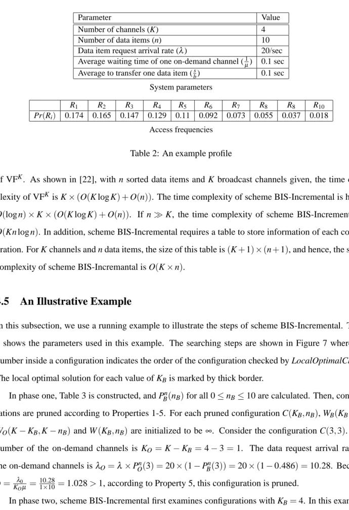
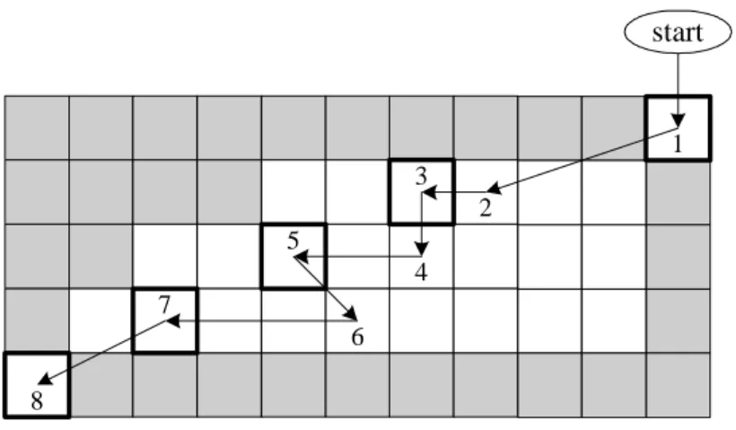
4.5 An Illustrative Example

In this subsection, we use a running example to illustrate the steps of scheme BIS-Incremental. Table 2 shows the parameters used in this example. The searching steps are shown in Figure 7 where the number inside a configuration indicates the order of the configuration checked by LocalOptimalCheck.

The local optimal solution for each value of K_Bis marked by thick border.

In phase one, Table 3 is constructed, and P_Bⁿ(n_B) for all 0 ≤ n_B≤ 10 are calculated. Then, configu- rations are pruned according to Properties 1-5. For each pruned configuration C(K_B, n_B), W_B(K_B, n_B), W_O(K − K_B, K − n_B) and W (K_B, n_B) are initialized to be∞. Consider the configuration C(3, 3). The number of the on-demand channels is K_O= K − K_B = 4 − 3 = 1. The data request arrival rate of the on-demand channels isλO=λ^{× P}_Oⁿ(3) = 20 × (1 − P_Bⁿ(3)) = 20 × (1 − 0.486) = 10.28. Because ρ⁼ _K^λ_O⁰_µ ⁼ ^10.28_1×10= 1.028 > 1, according to Property 5, this configuration is pruned.

In phase two, scheme BIS-Incremental first examines configurations with K_B= 4. In this example,