CSI Feedback for Closed-Loop MIMO-OFDM
Systems based on B-splines
Ren-Shian Chen
† and Ming-Xian Chang
Institute of Computer and Communication Engineering and Department of Electrical Engineering National Cheng-Kung University Tainan, 70101, Taiwan E-mail:†[email protected]
Abstract—In this paper, we propose a feedback algorithm based on the B-spline models of channel responses(CRs) variation across subchannels. We determine the coefficients of the B-splines based on the least-squares fitting principle. The coefficients of the B-splines are fed back to the transmitter for the CRs reconstruction. In the feedback process, we also apply efficient quantization algorithms based on the Gaussian quantization. The simulation results verify that the proposed B-spline model has smaller coefficients variances, and this leads to smaller mean-squares error than the Polynomial model [1] when using fewer number of feedback bits. The simulation results also show that the proposed algorithm can attain the upper bound of channel capacity for the precoded MIMO-OFDM system in the frequency-selective channel.
I. INTRODUCTION
The multiple-input multiple-output (MIMO) system with orthogonal frequency-division multiplexing (OFDM) transmis-sion is a robust scheme in the frequency-selective wideband fading channel. The MIMO system enhances the system capac-ity by exploiting the spatial diverscapac-ity, while the OFDM trans-mission enables the receiver the low-complexity frequency-domain equalization.
We can increase the system performance and capacity by the precoding of the transmitted signals. The well-known precoding systems include beamforming systems (BS) and multiplexing systems (MS). For the BS the transmitted signal is assigned an appropriate direction according to the chan-nel state information (CSI) of the MIMO system, such that we can decrease the interference or increase the received power [2]. The MS for MIMO-OFDM allocates power to different antennas or subchannels according to the CSI for adaptive communications [3] [4]. Due to the finite and precious bandwidth resource between the transmitter and receiver, we need to take into account the consumed power and quantity of the fed-back CSI.
For the MIMO channel, we can use vector quantizer (VQ) and matrix quantizer (MQ) [5]- [6] to implement the quanti-zation of beamforming vectors and matrices. A more practical MIMO system with the geodesic method that needs only 1 bit was proposed in [7], which can track the varying beamform-ing vectors and subspaces in the time-selective channel by the correlation between fed-back beamforming vectors. The frequency correlation can be exploited in the MIMO-OFDM system [8] [9] by cluster, recursive and trellis-based methods,
respectively, to reduce the feedback load.
However, for a system with power allocation at the trans-mitter, there are few discussions about the extra gain from the feedback of channel responses (CRs), which are also the essential part of the CSI. In an MIMO-OFDM system with Nc
subchannels, for each transceiver antenna pair, the receiver needs to feed back NcBc bits to the transmitter during the
time slot of one OFDM symbol, where Bc is the number of
quantization bits for the CR of each subchannel.
In this paper, we propose a parametric method to reduce the feedback load of CRs in the MIMO-OFDM system. The proposed parametric method is based on the B-spline model, and the performance is compared with the regression polynomial model in [1]. We consider the frequency selective fading channel and model the variation of CRs across sub-carriers by B-splines. The coefficients, which are served as the parameters of the CRs, are determined by the least-squares fitting (LSF) principle [11]. The transmitter can rebuild the CRs based on the fed-back B-spline coefficients. To efficiently return the coefficients, we need to further apply quantization. Due to the complex Gaussian distribution of the CRs, the coefficients of the B-splines also have the complex Gaussian distribution. Therefore, we apply the Gaussian quantization (GQ) after the coefficients of the B-splines are determined. Due to the smaller variance of the coefficients, the simulation shows that the B-spline model attains better performance than the Polynomial model [1] when we use smaller number of feedback bits. Under the reasonable feedback load, the simulations also shows that by the proposed algorithm the channel capacity can approach the upper bound, which is obtained by using the true CRs.
The rest of this paper is organized as follows. In Section II, we give a brief introduction of B-spline-based parametrization of CRs and the LSF approach. In Section III, we analyze the variance of coefficients in the B-spline model. Section IV gives the simulation results. Finally, the we conclude this paper in Section V.
Notation : Bold upper and lower letters denote matrices and
column vectors, respectively. We use (·)T and E(·) to denote transpose and expectation, respectively, and CN (µ, σ2) the complex Gaussian distribution with mean µ and variance σ2. The (i, j)th element of a matrix A is denoted by A(i, j).
II. PARAMETRIZATION OFCSI
For each pair of MIMO transceiver, since the CRs are correlated among neighboring subchannels, we can develop efficient approaches to feed back the estimated CRs in the receiver to the transmitter. We assume the CRs among different transceiver antennas are independent. In the following, we first briefly introduce the B-splines, then we use B-splines to model the CRs variation across the subchannels of the MIMO-OFDM system. The coefficients of the B-splines are quantized and fed back such that the transmitter can reconstruct the CRs.
A. The B-splines
A B-spline of order n, denoted by Bn(t), is an n-fold
convolution of the B-spline of zero order Bo(t) [12]. For
n = 0, 1, 2 we have the following B-splines.
Bo(t) = 1, −T2 <|t| < T2, 1 2, |t| = T 2, 0, otherwise. (1) B1(t) = { 1−|t|T, |t| < T2, 0, otherwise. (2) B2(t) = 3 4− t2 T2, |t| < T 2, t2 2T2 − 3|t| 2T + 9 8, T 2 ≤ |t| < 3T 2 , 0, otherwise. (3)
B. Model the CRs Variation across Subchannels
Now we use B-splines to model the channel variation across subchannels piecewisely in OFDM systems. The co-efficients of B-splines are determined based on the least-squares fitting (LSF) approach. In the modeling process, we transform Nc estimated CRs of subchannels into B-spline
coefficients. The receiver then feeds back these coefficients to the transmitter for the reconstruction of CRs. More precisely, let h = [H1, ..., HNc]
T, where H
k is the CR of the kth
subchannels at some symbol time slot. We partition h into
Np segments, h = [hT1, ..., h T Np]
T with the ith segment
hi = [ H1+(i−1)Nc Np , ..., HiNc Np ]T , 1≤ i ≤ Np.
In this paper, we choose n = 2 and use B2(t) as the
fitting curve. The receiver uses m B2(t) to fit each hi. On
each B2(t), we sample q points, where the parameter q is
determined by q + (m− 1)q 2 ∼= Nc Np . (4)
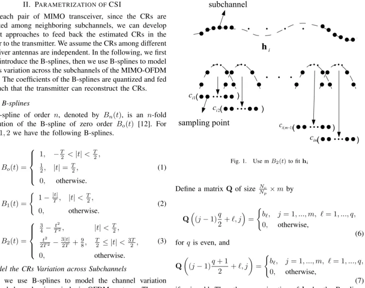
As indicated in Fig. 1, each sample is multiplying a proper coefficient to fit hi. Let b = [b1, ..., bq]T, where bℓ is the ℓth
sampling point from B2(t), or
bℓ= B2 ( −3T 2 + ℓ( 3T q + 1) ) , ℓ = 1, ..., q. (5)
Fig. 1. Use m B2(t) to fit hi
Define a matrix Q of size Nc
Np× m by Q ( (j− 1)q 2+ ℓ, j ) = { bℓ, j = 1, ..., m, ℓ = 1, ..., q, 0, otherwise, (6) for q is even, and
Q ( (j− 1)q + 1 2 + ℓ, j ) = { bℓ, j = 1, ..., m, ℓ = 1, ..., q, 0, otherwise, (7) if q is odd. Then the approximation of hi by the B-splines
B2(t)’s fitting can be expressed as
ˆ
hi= Qci, ci= [ci1, ..., cim]T, (8)
where cij means the j-th coefficient in hi, j = 1, ..., m. The
coefficients vector ciis determined by the least-squares-fitting
principle such that each∥hi− ˆhi∥2 is minimized,
min ci ∥h
i− Qci∥2. (9)
We can solve the coefficients vector ci as
ci= (QTQ)−1QThi= Phi, (10)
where the matrix P = (QTQ)−1QT.
After ci’s are determined, the receiver can feed back these
ci’s to the transmitter with the quantization process. The
number of feedback coefficients for each OFDM block h is
Npm, which is usually much smaller than Nc, the original
number of CRs on the subchannels. For an MIMO-OFDM systems with Nt transmit antennas and Nr receive antennas,
TABLE I
POLYNOMIAL COEFFICIENT’S VARIANCE, Np= 4,DEG=4 .
cij j = 1 j = 2 j = 3 j = 4
i = 1 9.1247e-1 2.8989e-2 2.5646e-4 5.6667e-6 i = 2 9.0016e-1 2.8606e-2 2.5286e-4 5.7075e-6 i = 3 9.1479e-1 2.8781e-2 2.5429e-4 5.7079e-6 i = 4 9.0283e-1 2.8514e-2 2.5175e-4 5.6629e-6 Ideal 9.1355e-1 2.9318e-2 2.5896e-4 5.7910e-6 DEG: polynomial order in [1] Ideal: calculated by (11)
TABLE II
B-SPLINE COEFFICIENT’S VARIANCE, Np= 4, m = 4.
cij j = 1 j = 2 j = 3 j = 4
i = 1 2.4853e-0 1.6288e-0 2.2383e-0 2.9236e-0 i = 2 2.4274e-0 1.6362e-0 2.2520e-0 2.9138e-0 i = 3 2.4390e-0 1.6082e-0 2.2033e-0 2.8819e-0 i = 4 2.4183e-0 1.6134e-0 2.2277e-0 2.9353e-0 Ideal 2.4505e-0 1.6216e-0 2.2325e-0 2.9297e-0
Ideal: calculated by (11)
III. COEFFICIENTANALYSE ANDGAUSSIAN
QUANTIZATION A. The Analysis of Coefficient Variance
After the modeling of CRs, we can feed back the coeffi-cients of the B-splines to transmitter. To implement efficient feedback, we need to quantize the coefficients. As we will show, the variations of coefficients have a great impact on the feedback load. Through the constant matrix P in (10), each element of cialso has complex Gaussian distribution with zero
mean and variance [13]
σc2 i(m)= N∑c−1 x=0 N∑c−1 y=0 P (m, x)P (m, y)E{si(x)si(y)} = L∑p−1 z=0 N∑c−1 x=0 N∑c−1 y=0 α2zP (m, x)P (m, y) cos ( 2π(x− y) z Nc ) (11) and σ2ℜ{c i(m)}= σ 2 ℑ{ci(m)}= 0.5σ 2 ci(m), (12)
whereℜ{ci(m)} and ℑ{ci(m)} denote the real and imaginary
parts of ci(m), respectively. In (11), αzdenotes the path gain
of the zth path, and Lp is the number of paths in channel.
By (11) and with simulations, we can find out the co-efficient’s variance. In Table I and Table II we give the variances of the coefficients of Polynomial [1] and B-splines, respectively, in the CRs modeling. We observe that the varia-tion of B-spline’s coefficients are more smooth than those of Polynomials.
B. Gaussian Quantization
After the parametrization, since the coefficients are complex Gaussian distributed, the Gaussian quantization (GQ) algorithm can be applied before the feedback. The GQ algorithm is based on two primary conditions, the nearest neighborhood condition (NNC) and the centroid condition (CC), to construct the optimization of the codebook and
decrease the distortion of quantization.
Assume Bc bits are used in the feedback, and N = 2Bc.
Let ˆck denote the center of the kth partition cell, 1≤ k ≤ N.
For a given large number of cj’s, we determine ˆck as follows.
NNC: The optimum partition cells satisfy
Rk={c : |ˆck− c| ≤ |ˆcj− c|, ∀k ̸= j} . CC: We determine ck by ˆ ck = N (R∑k) j=1 cjPcj, cj ∈ Rk,
where N (Rk) is the number of cj in Rk, and
Pcj is the probability of cj.
The quantization error is defined as
eQ= N ∑ k=1 N (R∑k) j=0 |ˆck− cj|Pcj . (13)
The two conditions are iterated until the quantization distor-tion eQconverges. For a given codebook,C = { ˆc1, ..., ˆc2Bc},
we determine the quantization point by ˆ
ck= arg min ˆ ck∈ C
|ˆck− cR|, (14)
where cR denotes the real part of an element of ci, and
similarly for the imaginary part element cIand ˆcI. Because of the coefficients have different variances; see (11), we need to quantize the coefficients by different codebooks. But we can transform the coefficients such that the distributions of coeffi-cients are the same. So we only have one standard codebook at the receiver and transmitter, and the transformation is given by ´ ci(m) = ci(m) √ σ2 ci(m) × σ2 std, (15)
where ´ci(m) is complex Gaussian distributed with zero mean
and variance σ2
std.
IV. NUMERICALRESULTS
We now give some numerical results to validate the pro-posed algorithms. We consider the Rayleigh fading channel based on IEEE 802.11 TGn model B with 9 taps and fdTs=
0.01, where fd is the maximum Doppler frequency shift and
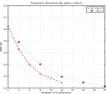
Tsis the OFDM symbol time. Fig. 2 and Fig. 3 show the the
parametric distortion of Polynomial [1] and B-spline models respectively for Np = 2, 4. It is clear that the Polynomial
model has smaller mean-squares error(MSEs). For Np= 2 and
DEG = m = 5, the receiver transforms the CRs of Nc= 64
subchannels into 10 coefficients, and the resulted MSEs (at the receiver) are 0.076 and 0.1845 for the Polynomial and B-spline modeling, respectively. In the quantization process, we use different number of feedback bits (Bc) to quantize each
2 4 6 8 10 12 14 16 18 20 10−3 10−2 10−1 100 Number of Coefficients MSE−Rx
Parametric Distortion (Polynomial)
Np=2 Np=4
Fig. 2. MSE of Polynomial distortion.
2 4 6 8 10 12 14 16 18 20 0.1 0.2 0.3 0.4 0.5 0.6 0.7 0.8 Number of Coefficients MSE−Rx
Parametric Distortion (B−spline−order2)
Np=2 Np=4
Fig. 3. MSE of B-spline distortion.
1 2 3 4 5 6 7 8
10−2
10−1
100 Polynomial v.s B−spline−order2 (Parametric + Quantized Distortion)
Bc
MSE−Tx
Polynomial(0.076)
B−spline−order2(0.1845)
Fig. 4. MSE with different number of feedback bits.
Fig. 4 shows the MSEs of the rebuilt CRs at the transmitter. Thought the B-spline model has larger parametric distortion comparing with the Polynomial model in Fig. 2 and Fig. 3, we observe in Fig. 4 that for lower Bc the B-spline model has
smaller reconstructed MSEs at the transmitter. We can attribute this to the smaller variance of the coefficients in the B-spline model than in the Polynomial model, as shown in Table I and Table II.
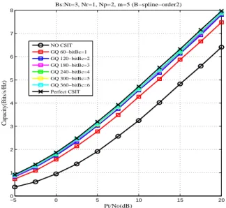
Next we consider an MIMO-OFDM BS system [14] with QPSK modulation, and the transmitter applies beamforming based on the fedback CRs with GQ. We show the bit-error rate
(BER) in Fig. 5 and Fig. 6. We note that when the number of feedback bits is less than 4, the B-spline model obtains better performance than the Polynomial model. Even when the feedback bits are increased, the performance of the B-spline model is almost the same as the Polynomial model. We also note that for the B-spline model, the BER is no longer reduced when the number of the feedback bits is more than 3. This verifies the B-spline can reach good performance with low feedback load. Fig. 7 shows the channel capacity of an MIMO-OFDM beamforming system. The upper bound is given by the case with the ideal water-filling principle and the true CRs. We observe that for the proposed feedback algorithm, the resulted channel capacities approach the upper bound.
V. CONCLUSION
In this paper, we propose efficient CRs feedback approach for the MIMO-OFDM system based on the B-spline model. We compare the performance of the proposed algorithm with the approach that is based on the Polynomial model. The simulation results validate that the proposed algorithm has better performance when we use smaller numbers of fed-back bits. The proposed algorithm can attain the upper bound of system capacity with low feedback load in the frequency-selective channel for the MIMO-OFDM system. We need not to use B-splines of higher order, since this increases the complexity but the performance improvement is limited.
REFERENCES
[1] S.-L. Chiou, K.-W. Hsieh, and M.-X. Chang, “Csi reduction of mimo-ofdm systems by parameterization,” in Proc. IEEE 19th International
Symposium on Personal, Indoor and Mobile Radio Communications, 2008. PIMRC 2008., 15-18 Sept 2008, pp. 1–5.
[2] S. Zhou and G. B. Giannakis, “Optimal transmitter eigen-beamforming and space-time block coding based on channel mean feedback,” IEEE
−2 0 2 4 6 8 10 12 10−5 10−4 10−3 10−2 10−1 100 Bs:Nt=3, Nr=1, Np=2, DEG=5 (Polynomial) Eb/No(dB) BER GQ 60−bitBc=1 GQ 120−bitBc=2 GQ 180−bitBc=3 GQ 240−bitBc=4 GQ 300−bitBc=5 Perfect CSIT
Fig. 5. Error performance of MIMO-OFDM beamforming systems with GQ. −2 0 2 4 6 8 10 12 10−5 10−4 10−3 10−2 10−1 100 Bs:Nt=3, Nr=1, Np=2, m=5 (B−spline−order2) Eb/No(dB) BER GQ 60−bitBc=1 GQ 120−bitBc=2 GQ 180−bitBc=3 GQ 240−bitBc=4 GQ 300−bitBc=5 Perfect CSIT
Fig. 6. Error performance of MIMO-OFDM beamforming systems with GQ. −50 0 5 10 15 20 1 2 3 4 5 6 7 8 Bs:Nt=3, Nr=1, Np=2, m=5 (B−spline−order2) Pt/No(dB) Capacity(Bits/s/Hz) NO CSIT GQ 60−bitBc=1 GQ 120−bitBc=2 GQ 180−bitBc=3 GQ 240−bitBc=4 GQ 300−bitBc=5 GQ 360−bitBc=6 Perfect CSIT
Fig. 7. Capacity of MIMO-OFDM beamforming systems with GQ.
[3] H. Sampath, P. Stoica, and A. Paulraj, “Generalized linear precoder and decoder design for mimo channels using the weighted mmse criterion,”
IEEE Trans. Commun, vol. 49, no. 12, pp. 2198 – 2206, Dec. 2001.
[4] A. Scaglione, P. Stoica, S. Barbarossa, G. B. Giannakis, and H. Sampath, “Optimal designs for space-time linear precoders and decoders,” IEEE
Trans. Signal Process, vol. 50, no. 5, pp. 1051 – 1064, May. 2002.
[5] J. C. Roh and B. D. Rao, “Transmit beamforming in multiple-antenna systems with finite rate feedback: a vq-based approach,” IEEE Trans.
Inf. Theory, vol. 52, no. 3, pp. 1101 – 1112, March 2006.
[6] B. D. Rao and J. C. Roh, “Design and analysis of mimo spatial multiplexing systems with quantized feedback,” IEEE Trans. Signal
Process, vol. 54, no. 8, pp. 2874 – 2886, Aug. 2006.
[7] J. Yang and D. B. Williams, “Transmission subspace tracking for mimo systems with low-rate feedback,” IEEE Trans. Commun, vol. 55, no. 8,
pp. 1629 – 1639, Aug. 2007.
[8] H. Zhang, Y. G. Li, V. Stolpman, and N. V. Waes, “A reduced csi feedback approach for precoded mimo-ofdm systems,” IEEE Trans.
Wireless Commun, vol. 6, no. 1, pp. 55 – 58, Jan. 2007.
[9] S. Zhou, B. Li, and P. Willett, “Recursive and trellis-based feedback reduction for mimo-ofdm with rate-limited feedback,” IEEE Trans.
Wireless Commun, vol. 5, no. 12, pp. 3400 – 3405, December. 2006.
[10] R. W. Heath, Jr., and D. J. Love, “Multimode antenna selection for spatial multiplexing systems with linear receivers,” IEEE Trans. Signal
Process, vol. 53, no. 8, pp. 3042 – 3056, Aug. 2005.
[11] M.-X. Chang and Y. T. Su, “Model-based channel estimation for ofdm signals in rayleigh fading,” IEEE Trans. Commun, vol. 50, no. 4, pp. 540 – 544, April. 2002.
[12] Y. V. Zakharov and T. C. Tozer, “Local spline approximation of time-varying channel model,” Electronics Letters, vol. 37, no. 23, pp. 1408 – 1409, Nov. 2001.
[13] M.-X. Chang and Y. T. Su, “Performance analysis of equalized ofdm systems in rayleigh fading,” IEEE Trans. on Wireless Commun, vol. 1, no. 4, pp. 721 – 732, Oct. 2002.
[14] J. Choi and R. W. H. Jr., “Interpolation based transmit beamforming for mimo-ofdm with limited feedback,” IEEE Trans. Signal Process, vol. 53, no. 11, pp. 4125 – 4135, Nov. 2005.
[15] M. Borgmann and H. Bolcskei, “Interpolation-based efficient matrix inversion for mimo-ofdm receivers,” in Conference Record of the
Thirty-Eighth Asilomar Conference on Signals, Systems and Computers, 2004,