國立臺灣大學理學院地理環境資源學系 碩士論文
Department of Geography College of Science
National Taiwan University Master Thesis
由 GPS 速度場之群聚分析來探討台灣的活動構造分區 Using Cluster Analysis of GPS Velocities to Explore
Active Tectonics in Taiwan
李依倢 Yi-Chieh Lee
指導教授:莊昀叡 博士 Advisor: Ray Y. Chuang, Ph.D.
中華民國 109 年 06 月 June, 2020
Abstract
GPS observations on the surface are commonly used for analyzing crustal deformation and active faults in such a way that surface velocities derived from GPS are often considered to be associated with fault movement at depths bounding rigid tectonic blocks. However, the choice of the tectonic blocks highly depends on either the knowledge of active fault geometries based on available field investigations and seismicity distribution or subjective determination from geodetic observations. To provide a more objective choice of blocks, cluster analysis is a useful tool, which groups a set of GPS velocities based on spatial statistics. Clusters can represent blocks and cluster boundaries and may reflect block-bounding faults. Under the arc-continent collision and mountain building, most of active faults in Taiwan are thrust faults or oblique faults. Therefore, it is crucial to examine how cluster analysis applied to the Taiwan region.
In order to examine the feasibility and characteristics of the cluster analysis for such thrust-dominant areas, this study used the K-medoids clustering algorithm for horizontal GPS velocities in Taiwan and estimate optimal block numbers by statistical methods of Elbow, Average silhouette, and gap statistic methods. The optimal cluster number is 4 and the analysis can estimate up to 34 clusters with discernible geologic features. Earlier determined clusters represent higher velocity gradient between the clusters, which may indicate active structures with higher slip rates. The cluster analysis can offer a simple and fast method to indicate the possible tectonic blocks and uncertain active structures.
Acknowledgement
I would like to thank my advisor, Dr. Ray Y. Chuang, and five committee members of my proposal defense and thesis defense: Dr. Wu-Lung Chang, Dr. Kuo‐En Ching, Dr.
J. B. H. Shyu, Dr. Tzai-Hung Wen, and Dr. Bing-Sheng Wu, who provide helpful suggestions and insightful comments for my thesis. I would like to thank Dr. Horng- Yue Chen of the GPS-LAB of the Institute of Earth Sciences, Academia Sinica, Taiwan (http://gps.earth.sinica.edu.tw), for providing the GPS data. I also thank Dr. J. B. H.
Shyu and the Central Geological Survey for providing shapefiles of active faults in Taiwan.
During my research, progressive results were presented at the following conferences and meetings: the 2018 Annual Meeting of The Geography Society of China Located in Taipei, 2018 Annual Meeting of the Geodetic Society of the Republic of China Conference, 2018 Taiwan-Japan-New Zealand Seismic Hazard Workshop, 2019 Taiwan Geosciences Assembly and 2019 AGU Fall Meeting. These travels are partially supported by the Travel Grant for Attending International Conferences, College of Science, NTU, and International Travel Grants, Research Center for Future Earth, NTU.
Two other grants, NTU International Scholarship for Visiting Partner Schools and MOE Pilot Overseas Scholarship, also support my visit to the Disaster Prevention Research Center, Kyoto University and the Department of Earth and Atmospheric Sciences, Indiana University, respectively. During my visit, I would like to thank Dr.
Takuya Nishimura, Dr. Kaj Johnson, and Dr. Michael W. Hamburger for useful comments.
This research is supported by the Ministry of Science and Technology with the grant number of 107-2116-M-002-021-MY2 and Taiwan Earthquake Research Center.
This research aims to be written in manuscript and submitted to an international journal
with coauthors of Dr. Ray Y. Chuang and Dr. Horng-Yue Chen.
I would like to express sincere gratitude to my advisor, Ray, who always encourages me and gave me advice when I felt helpless and trapped in the problem.
Thank you for accepting me when I had no places to go and spent your time teaching me. I would also thank the whole members in lab 303. Thanks to Shonjay and Penny who always share your warm shoulders with me and encourage me when I felt upset.
Thanks to Chia-Ying who introduced me to Ray and open a new page in my life. Thanks to Zax, Chelsey, Max, and Fox who always can give me the most objective and useful advice about the research. Thanks to Evan, Kevin, and Jack who gave me a lot of interesting time every day. Certainly, I would not forget my weight training partner, Yu- Fang, my shopping partner, Wan-Tzu and Amy. I will never forget those countless sleepless nights we were working hard together for the meeting or for the research, and for all the interesting things we have experienced together in these years. Without any of you, I cannot finish this thesis smoothly and have such a meaningful time during my graduate period.
Last but not the least, I would like to thank my parents and my sister for their encouragement and support in spirit and material in these years. I also thank my dearest friends, Yaya Jian, Yuan-Ping, Yashiou, Jia-Ru, Shelly Wu, Yi-Cheng, and my college classmates, Jane Yang, Vicky Chen, Howard Huo, Rong-Jin, Elaine Chen, Dong-Xian, Chia-Che, Hong-Shen, Yi-De, An-Soon, Chi-Wen, Chi-Chieh, and Yuan-Fu. Thank you for always stand by my side and support me. Without you, I would not achieve all of the accomplishments. I sincerely thank everyone who has appeared in my life and love all of you, always.
Table of Contents
Chapter 1 Introduction ... 1
Chapter 2 Tectonic settings of Taiwan ... 5
2.1 Tectonic background ... 5
2.2 Active Structures in Taiwan ... 10
Chapter 3 Reviews of methodology ... 17
3.1 Interseismic Velocity derived from GNSS ... 17
3.2 Cluster Analysis ... 19
3.3 Statistical Test ... 23
3.4 Cluster analysis in the application of active tectonics ... 25
Chapter 4 Data and Methods ... 29
4.1 Pre-process Tests ... 34
4.1.1 Reference frame ... 34
4.1.2 Velocity Distribution ... 38
4.2 Threshold for Stopping ... 40
Chapter 5 Result ... 41
5.1 Taiwan ... 42
5.1.1 4 clusters ... 42
5.1.2 10 clusters ... 43
5.2 Local area ... 45
5.2.1 Northern Taiwan ... 47
5.2.2 Western Taiwan ... 50
5.2.3 Eastern Taiwan ... 52
5.2.1 Southwestern Taiwan ... 56
5.3 Clustering result for each k ... 58
Chapter 6 Discussion ... 79
6.1 Clustering result for whole Taiwan ... 79
6.2 Tectonic Implications ... 84
6.2.1 Northern Taiwan ... 84
6.2.2 Western Taiwan ... 85
6.2.3 Eastern Taiwan ... 88
6.2.4 Southwestern Taiwan ... 92
6.3 Implications for Fault-Slip Rates and Seismic Potential ... 95
6.4 Compare to the Block Model ... 101
Chapter 7 Conclusions ... 107
References ... 109
Appendix 1: The statistic result of the Gap Statistic ... 123
List of Figures
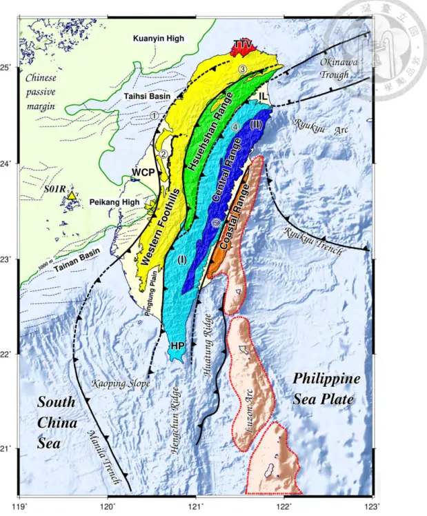
Figure 1 The tectonic settings of Taiwan. The yellow area is the Western Foothills, the green area is the Hsuehshan Range, the blue area is the Central Range, the brown area is the Coastal Range and the Yellow triangle presents the locations of reference GPS station. WCP: Western Coastal Plain; TTV: Tatun Volcanoes; HP:
Hengchun peninsula; IL: Ilan plain. Numerals 1–5 indicate the deformation front, the Chelungpu fault, the Chihtsu fault, the Lishan fault, and the Longitudinal Valley fault (Ching et al., 2011b). ... 8 Figure 2 The map of the major active faults and folds of Taiwan. There are seven domains along the western belt and four along the eastern, each domain is defined by the distinctive active structures (Shyu, 2005). ... 9 Figure 3 The active fault map of Taiwan which announced by Central Geological Survey (CGS). ... 11 Figure 4 The major seismogenic structures of Taiwan which provided by Shyu, J. Bruce H., and the blue lines show the 45 structures in Taiwan. ... 12 Figure 5 Active structures in Taiwan which announced by C.G.S (2012) and TEM (provided by Shyu, J. Bruce H.). ... 15 Figure 6 The 492 continuous GPS stations used in this research. ... 30 Figure 7 The horizontal GPS velocity fields of Taiwan, relative to IGS08. ... 31 Figure 8 GPS velocity fields for Taiwan. The left one is the original version and the right one is the velocity field which is separated by cluster algorithm. Different colors mean different blocks in Taiwan, the green cluster means the Coastal Range, the blue cluster means the Pingtung Plain, the orange cluster means the Western Foothills and the purple cluster means the Eurasian continental margin. ... 32 Figure 9 Velocity fields relative to ITRF and S01R reference frames. The blue one is relative to the ITRF reference frame and the green one is relative to the S01R
station. ... 36 Figure 10 Clustering result of different reference frames. Different color means different groups. (a) is the GPS velocity field relative to ITRF which presented as an arrow, (b) is the result of Figure 10a after cluster which presented as point, (c) is the GPS velocity field relative to S01R which presented as an arrow, and (d) is the result of Figure 10c after cluster which presented as point. The same color represents the same group ... 37 Figure 11 Velocity setting of the synthetic data which is 10 by 10 grid. The left one means the velocity of each blocks and the right one means different groups. The velocity of the stations in the green block is 10, in the pink block is 20, in the orange block is 30, and in the purple block is 40. ... 39 Figure 12 The result after random selection. The value at the lower-left means the numbers of the station which chooses in this test. ... 39 Figure 13 Statistic results for Taiwan. The orange line is the result of the elbow method, the blue line is the result of the average silhouette method, and the green line is the gap statistic result. The dashed line is the significant turning point which indicates the optimal number for the clustering result. ... 42 Figure 14 Clustering result for whole Taiwan when k = 4. ... 43 Figure 15 Clustering result for whole Taiwan when k = 10. ... 44 Figure 16 Four domains in Taiwan. I: Northern Taiwan; II: Western Taiwan; III:
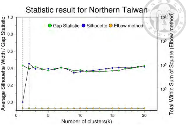
Southwestern of Taiwan; IV: Eastern Taiwan. The black line is the active structures announced by the CGS and TEM. ... 46 Figure 17 Statistic result for Northern Taiwan. The dash line at k = 1 and 2 is the optimal number of blocks which calculated by the gap statistic method and average silhouette method, respectively. ... 48 Figure 18 The clustering result of northern Taiwan by the gap statistic method. ... 49
Figure 19 The clustering result of northern Taiwan by the average silhouette method.
... 49
Figure 20 Statistic result for Western Taiwan. The dash line at k = 2 and 3 is the optimal number of blocks which calculated by the gap statistic method and average silhouette method, respectively. ... 50
Figure 21 The clustering result of western Taiwan by the gap statistic method. ... 51
Figure 22 The clustering result of western Taiwan by the average silhouette method. ... 52
Figure 23 Statistic result for Eastern Taiwan. The dash line at k = 3 is the optimal number of blocks which calculated by the gap statistic method and average silhouette method. ... 53
Figure 24 The clustering result of eastern Taiwan by the gap statistic method. ... 54
Figure 25 The clustering result of eastern Taiwan by the average silhouette method. 55 Figure 26 Statistic result for Southwestern Taiwan. The dash line at k = 2 and 7 is the optimal number of blocks which calculated by the gap statistic method and average silhouette method, respectively. ... 56
Figure 27 The clustering result of southwestern Taiwan by the gap statistic method. 57 Figure 28 The clustering result of southwestern Taiwan by the average silhouette method. ... 57
Figure 29 Clustering result for Taiwan in k = 5. ... 63
Figure 30 Clustering result for Taiwan in k = 6. ... 63
Figure 31 Clustering result for Taiwan in k = 7. ... 64
Figure 32 Clustering result for Taiwan in k = 8. ... 64
Figure 33 Clustering result for Taiwan in k = 9. ... 65
Figure 34 Clustering result for Taiwan in k = 10. ... 65
Figure 35 Clustering result for Taiwan in k = 11. ... 66
Figure 36 Clustering result for Taiwan in k = 12. ... 66
Figure 37 Clustering result for Taiwan in k = 13. ... 67
Figure 38 Clustering result for Taiwan in k = 14. ... 67
Figure 39 Clustering result for Taiwan in k = 15. ... 68
Figure 40 Clustering result for Taiwan in k = 16. ... 68
Figure 41 Clustering result for Taiwan in k = 17. ... 69
Figure 42 Clustering result for Taiwan in k = 18. ... 69
Figure 43 Clustering result for Taiwan in k = 19. ... 70
Figure 44 Clustering result for Taiwan in k = 20. ... 70
Figure 45 Clustering result for Taiwan in k = 21. ... 71
Figure 46 Clustering result for Taiwan in k = 22. ... 71
Figure 47 Clustering result for Taiwan in k = 23. ... 72
Figure 48 Clustering result for Taiwan in k = 24. ... 72
Figure 49 Clustering result for Taiwan in k = 25. ... 73
Figure 50 Clustering result for Taiwan in k = 26. ... 73
Figure 51 Clustering result for Taiwan in k = 27. ... 74
Figure 52 Clustering result for Taiwan in k = 28. ... 74
Figure 53 Clustering result for Taiwan in k = 29. ... 75
Figure 54 Clustering result for Taiwan in k = 30. ... 75
Figure 55 Clustering result for Taiwan in k = 31. ... 76
Figure 56 Clustering result for Taiwan in k = 32. ... 76
Figure 57 Clustering result for Taiwan in k = 33. ... 77
Figure 58 Clustering result for Taiwan in k = 34. ... 77
Figure 59 Clustering result in Taiwan at k =4. The black solid line is the surface traces of the known active fault. PH: Philippines; EU: Eurasian Plate; PT: PingTung; NA: NAnao (Takahashi et al., 2019). ... 82
Figure 60 Clustering result in Taiwan at k =11. The black solid line is the surface traces of the known active fault. PH: Philippines; NA: NAnao; PT: PingTung; WF:
Western Foothills; WPT: West PingTung; LUZ: Luzon Arc; KS: KaohSiung; TW:
TaiWan; IL: Ilan; CeR: Central Range; CoR: Coastal Range (Takahashi et al.,
2019). ... 83
Figure 61 Cluster result when k = 34 in northern Taiwan. ... 85
Figure 62 Cluster result when k = 34 in western Taiwan. ... 88
Figure 63 Cluster result when k = 34 in eastern Taiwan ... 91
Figure 64 Cluster result when k = 34 in southwestern Taiwan. ... 94
Figure 65 Cluster order map of Taiwan. The dark color means that cluster boundaries are identified earlier, and vice versa. ... 97
Figure 66 The relationship between the cluster order defined in this study and the slip rate. The X-axis is the cluster order, the smaller number means that structures be identified earlier, and vice versa. The Y-axis is the slip rate calculated by Shyu et al. (2016). The label of each data point means the name of the fault and its slip rate. ... 98
Figure 67 The map of geologic slip rate which calculated by Shyu et al. (2016) with the clustering result for k = 4. ... 100
Figure 68 Compare the previous block model used in Ching et al. (2011c) with the 4 clusters in this study. EURA: Eurasian Plate; I‐a: Deforming domain in SW Taiwan; I‐b: quasi‐rigid block domain in SW Taiwan; II‐a, II‐b: central domain; III‐a: Waning collision zone; III‐b: Outer range of the transition zone; III‐c: Inner range of the transition zone; IV: Eastern Taiwan; V: the Central Range. ... 102
Figure 69 Compare the previous block model used in Ching et al. (2011c) with the 34 clusters in this study. The meanings of the color are as same as Figure 68. ... 103 Figure 70 Compare to the previous block model used in Chang et al. (2016) with the 4
clusters in this study. Chang et al. (2016) separated Taiwan into 34 blocks with 27 known active faults as their boundaries. ... 104 Figure 71 Compare to the previous block model used in Chang et al. (2016) with the 34 clusters in this study. Chang et al. (2016) separated Taiwan into 34 blocks with 27 known active faults as their boundaries. ... 105
List of Table
Table 1 GPS stations in each domain. ... 45 Table 2 RGB value of each cluster. ... 61 Table 3 The Gap statistical result for Taiwan ... 123
Chapter 1 Introduction
Geodetic observations are useful for analyzing fault geometries and behaviors, which are crucial for active tectonics and seismic hazard assessments. In order to analyze present-day surface velocities in three dimensions (3D), block models are commonly used to describe interseismic deformation according to block tectonics (McCaffrey, 2005;
Meade and Hager, 2005), which is based on the motion characteristics of the same block should be extremely similar. For this reason, when the distribution of tectonic blocks and active faults is less certain, cluster analysis of surface velocities derived from GPS provides an objective way to identify clusters with similar movement patterns, which can help differentiate block geometries (Simpson et al., 2012).
The method of cluster analysis for GPS velocities can estimate the number of blocks and block boundaries, and it has been applied to plate boundary zones such as California (Simpson et al., 2012; Savage and Simpson, 2013a, b; Thatcher et al., 2016), western U.S.
(Savage and Wells, 2015), and Japan (Savage, 2018). Simpson et al. (2012) used the hierarchical agglomerative clustering for GPS velocities to search for the spatial coherent of the crustal deformation around the San Francisco area. Savage and Simpson (2013a), Savage and Simpson (2013b), Savage and Wells (2015), and Thatcher et al. (2016) used the K-medoids clustering with Euler vectors to take account of the effect of the rotation
blocks, which treat the Earth as a sphere rather than a plane. The studies above focused on evaluating the feasibility of identified the crustal blocks without any prior geologic information through the clustering algorithms. Afterwards, Savage (2018) used the Euler- vector clustering for southwest Japan and compare the result with proposed microplate geometry. Recently, Takahashi et al. (2019) applied the hierarchical clustering for the Taiwan and introduced the information entropy to quantify the significance and the stability of the cluster boundaries. The previous studies have proved that cluster analysis is helpful to discuss some tectonic significance, especially in the region where the geological background is still unclear.
As a young orogenic belt under the arc-continental collision between the Eurasian and Philippine Sea plates (Teng, 1990; Byrne et al., 2011), the island of Taiwan has been a spotlight for studies of its active tectonics. The division of tectonic blocks and domains as well as the identification of active structures are important for understanding tectonic processes (Lacombe et al., 2001; Shyu, 2005; Ching, 2007) and for block model configuration (Ching et al., 2011c; Chang et al., 2016). Takahashi et al. (2019) applied the clustering for the GPS velocity fields and distinguish 11 clusters in Taiwan, but the identified blocks are few and it is still unclear the relationship between clusters and tectonic blocks, and how the subsurface fault geometry can influence the results of cluster analysis under such a rapid, narrow fault-and-thrust belt.
To clarify these issues, this study uses the K-medoids algorithm of the centroid-based cluster analysis, which is more widely used in previous studies (Savage and Simpson, 2013a, b; Savage and Wells, 2015; Thatcher et al., 2016; Savage, 2018), to examine the relationship between clusters and active structures, which could help characterize the localities and activities of active structures within the plate-boundary deformation zone of Taiwan. It enables to understand the tectonic processes and provide another aspect of the configuration of the block models.
The structure of this thesis is described as following. Chapter 2 reviews the tectonic settings of the Taiwan island, which is the study area of this research. Chapter 3 summarizes the basic methodology of cluster analysis. Chapter 4 elaborates on the data and methods used in this research and Chapter 5 demonstrates the results. Chapter 6 discusses the clustering result between the previous study and this study (section 6.1), the implications of tectonic blocks (section 6.2), meaning of the seismic potential (section 6.3), and the comparison between the cluster analysis results and published block models (section 6.4).
Chapter 2 Tectonic settings of Taiwan
2.1 Tectonic background
The island of Taiwan has been forming and deforming under the orogenic process between the Eurasian and Philippine Sea plates. The NUVEL-1 plate motion model (Seno et al., 1993) and GPS observations (Yu et al., 1997; Yu et al., 1999) show that the Philippine Sea plate moves northwestwards at a rate of ~7-8 cm/a with respect to the Eurasian plate. As the South China Sea subducted and closed along the northern Malina Trench, the tectonic model of the collision between the Luzon Arc and Asian continental margin (Suppe, 1981; Suppe et al., 1987; Teng, 1990; Malavieille et al., 2002; Huang et al., 2006; Byrne et al., 2011) is widely favored although some alternative models such as the arc-arc collision were suggested (Hsu and Sibuet, 1995; Sibuet and Hsu, 1997).
With such tectonic environment, different models have been proposed to explain the creation of the current Taiwan orogenic system. The Longitudinal Valley is the main suture zone between the Coastal Range, part of the Luzon arc, to the east and the western mountains. The main mountains are considered to be accreted and they contain three geologic units from the east to west: the metamorphic Central Range, the Hsuehshan Range, and the active fold-and-thrust Western Foothills (Figure 1). The conventional arc- continent collision model views the Taiwan mountains and Hengchun Ridge are the
accretional prisms (Huang et al., 1997), but the geologic continuation between the Central Range, which contains pre-Cenozoic basement, and Hengchuan Ridge requires more detailed interpretations (Lu and Hsü, 1992; Shyu et al., 2005a). In addition, the deformation mechanism of the Taiwan orogen is interpreted differently. The common thin-skinned model suggests the Taiwan orogenic wedge is created above a main east- dipping detachment (Carena et al., 2002; Yue et al., 2005) based on the mechanism of Coulomb stress (Davis et al., 1983; Dahlen et al., 1984; Dahlen and Barr, 1989).
Considering the Central Range as part of the orogenic belt, the doubly-vergent model is also proposed to describe the critical wedge is supported by both the western fore-wedge and eastern retro-wedge detachments (Koons, 1990; Willett et al., 1993; Chuang et al., 2014). Furthermore, the presence of deeper earthquakes and structures inspired the interpretation of the thick-skinned model (Wu et al., 1997; Lin et al., 1998; Bertrand et al., 2009). With these inconsistent models, some studies suggest the coexistence of both thin- and thick-skinned models (Mouthereau and Lacombe, 2006; Huang et al., 2015).
In addition to the mountain building, other tectonic activities also shape some part of the island. In northern Taiwan, reversed subduction polarity (Suppe, 1984; Ustaszewski et al., 2012) caused normal faulting and mountain collapse (Teng, 1996). The subduction of the Ryukyu trench also results in the back-arc spreading of the Okinawa Trough (Wu, 1978; Letouzey and Kimura, 1986) and its westward propagation generated the opening
of the Ilan Plain (Hou et al., 2009). In southwestern Taiwan, the left-lateral fault along the eastern edge of the Pingtung Plain and a series of right-lateral faults around the northwestern plain suggest the activity of tectonic extrusion (Lacombe et al., 2001; Liu et al., 2004; Ching et al., 2007a; Hu et al., 2007). Moreover, mud diapirs could also play an important role in regional deformation in southwestern Taiwan (Hsieh, 1970; Chen et al., 2014b; Doo et al., 2015).
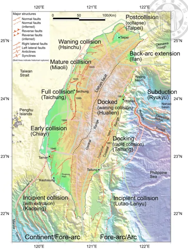
Since the geometric and deformational models vary, studies of tectonic domains and geometries of numerical models are different accordingly. According to the different collision stages, Shyu (2005) divided the island of Taiwan into 11 domains, which are dominated by different active structures (Figure 2). First-order cross-island deformation is analyzed and modeled independently following the thin-skinned model (Loevenbruck et al., 2001; Hsu et al., 2003; Simoes et al., 2012), doubly-vergent model (Willett et al., 2003; Whipple and Meade, 2004; Johnson et al., 2005; Whipple and Meade, 2006; Ching et al., 2011b), and thick-skinned model (Lin, 2000; Yamato et al., 2009). In a broader scale, the regional deformation of Taiwan is modeled block-wise according to the distribution of main structures (Hu et al., 2001; Bos et al., 2003; Ching et al., 2011c;
Chang et al., 2016).
Figure 1 The tectonic settings of Taiwan. The yellow area is the Western Foothills, the green area is the Hsuehshan Range, the blue area is the Central Range, the brown area is the Coastal Range and the Yellow triangle presents the locations of reference GPS station. WCP: Western Coastal Plain; TTV: Tatun Volcanoes; HP: Hengchun peninsula; IL: Ilan plain. Numerals 1–5 indicate the deformation front, the Chelungpu fault, the Chihtsu fault, the Lishan fault, and the Longitudinal Valley fault (Ching et al., 2011b).
Figure 2 The map of the major active faults and folds of Taiwan. There are seven domains along the western belt and four along the eastern, each domain is defined by the distinctive active structures (Shyu, 2005).
2.2 Active Structures in Taiwan
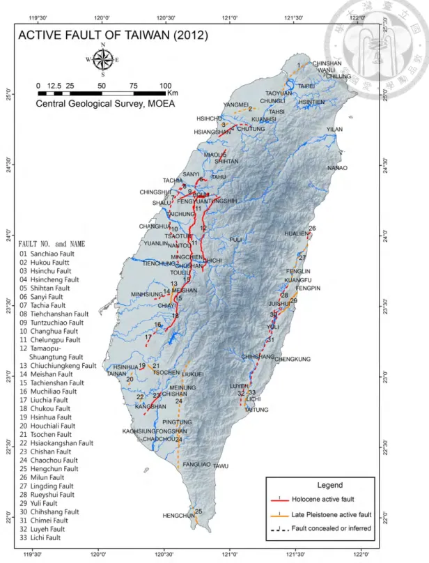
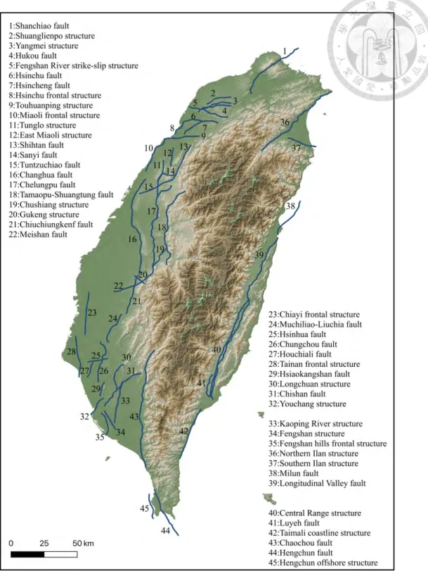
Since the processes of the subduction and mountain building control the deformation of the Taiwan island, active structures are generated under the tectonic forces to accommodate the relative plate motion across the island. These active structures highly influence local topography and seismic potential (Shyu et al., 2005b). The regional investigation of active faults in Taiwan started in 1970’s (Bonilla, 1975, 1977; Yang, 1986). In recent years, two maps of major active faults and structures were published by the Central Geological Survey (CGS) (Figure 3) and the Taiwan Earthquake Model (TEM) (Figure 4) (provided by Shyu, J. Bruce H.). Currently, CGS announced 33 active faults and 4 suspected active faults and TEM identified 45 on-land active structures.
The distribution of the active tectonics published by TEM and CGS are generally consistent and a few of them are different locally. Figure 5 shows the map of the active structures of CGS and TEM. In the Taipei area, the main active fault is the Shanchiao normal fault in response to the mountain collapse (Huang et al., 2007; Chen et al., 2014a).
Away from the extensional region and towards the orogenic belt, the Taoyuan area is dominated by the Pingchen and Hukou anticlines (Shyu et al., 2005b) and the Hsinchu area is affected by the Hsincheng and Hsinchu faults (Yang et al., 1996; Yang et al., 1997;
Chen et al., 2004).
Figure 3 The active fault map of Taiwan which announced by Central Geological Survey (CGS).
Figure 4 The major seismogenic structures of Taiwan which provided by Shyu, J.
Bruce H., and the blue lines show the 45 structures in Taiwan.
In central Taiwan, a series of folds are present in the Miaoli area and three major faults are distributed in the Taichung and Nantou areas. Surface ruptures of the 1935 Taichung-Hsinchu earthquake revealed two major faults around the Miaoli area: the Tuntzuchiao and Shihtan faults (Wang et al., 1994; Lin, 2005). Three sub-parallel faults including the surface rupture of the 1999 Chi-Chi earthquake are the Changhua (Yue et al., 2011), Chelungpu (Chen et al., 2001; Lee et al., 2003), and Tamaopu-Shuangtung faults. To the south, the Meishan fault is the surface rupture of the 1906 Meishan earthquake and the Liuchia-Muchiliao fault is the frontal active faults of the Western Foothills in Chiayi area. In addition, CGS listed the Chukou fault but TEM seems to consider it rather inactive. Instead, TEM identified the Chiayi frontal structure to explain regional uplift in the Chiayi plain (Shyu, 2005; Shyu et al., 2016).
In the Tainan and Kao-Ping areas, the TEM map (Figure 4) shows more active structures than CGS (Figure 3). The Hsinhua fault, which is the surface rupture of the 1946 Hsinhua earthquake, and the Houchiali fault, which is thought to be a backthrust east of the Tainan Tableland (Fruneau et al., 2001; Huang et al., 2006; Le Béon et al., 2019), are two major faults shown in both maps in Tainan. In the Kao-Ping area, the eastern Chaochou fault and western Chihshan fault are two major faults also shown in both maps. Moreover, the TEM map shows more minor structures such as the Longchuan fault, Chungchou structure, Fengshan structure, and so on.
In eastern Taiwan, the identified structures are fewer but rather important. The TEM map shows the Northern and Southern Ilan structure, corresponding to the northern and southern bounds of the back-arc spreading of the Okinawa Trough, respectively. In the Longitudinal Valley, the Milun fault, which is ruptured during the 1951 Hualien-Taitung and 2018 Hualien earthquakes (Huang et al., 2019; Lin et al., 2019; Yen et al., 2019), and Longitudinal Valley fault are located along the eastern edge of the valley. The Longitudinal Valley fault was partially ruptured during the 1951 earthquake (Shyu et al., 2007) and 2003 Chengkung earthquake (Wu et al., 2006a; Ching et al., 2007b; Kuochen et al., 2007). The southernmost Longitudinal Valley fault is partitioned into the eastern Peinan and western Luyeh faults (Lee et al., 1998; Shyu et al., 2008; Chuang et al., 2012).
On the other hand, the Central Range fault, which is located at the western valley, was ruptured in segment during the 2006 Taitung earthquake (Wu et al., 2006b), 2013 Rueisuei earthquake (Chuang et al., 2014), and 2018 Hualien earthquake (Lee et al., 2019).
Although current studies have generally consistent understanding of the active structures at a large scale, but in a local area there is still a large difference in the terms of the existence and geometry of the active structures. It is still uncertain about the distribution and the geometry of the fault that causes some problems to build the tectonic blocks model of Taiwan, which still highly depends on the knowledge of active tectonics and fault geometries and is limited by available data or structural interpretations. To
resolve this problem, this study aims to apply the cluster analysis for GPS velocities to analyze the active tectonics and tectonic domains in Taiwan.
Figure 5 Active structures in Taiwan which announced by C.G.S (2012) and TEM (provided by Shyu, J. Bruce H.).
Chapter 3 Reviews of methodology
3.1 Interseismic Velocity derived from GNSS
In 1973, the United States Department of Defense began to develop the Global Positioning System (GPS) for its military purposes. Through satellite radio navigation, it was able to provide the navigation services around the world, and then gradually opened up for civil use. In addition to the global positioning system of the United States, there are other similar systems developed in recent years such as the GLObal Navigation Satellite System (GLONASS) of Russia, the Galileo system of Europe Union, the BeiDou Navigation Satellite System of China and the Quasi-Zenith Satellite System (QZSS) of Japan.
The emergence of GPS has brought great breakthrough in the related research of crustal deformation. Using receivers on the ground can receive the ephemeris parameters and time information sent by more than four satellites to obtain the measurements of position, velocity and time (Sickle, 2015). However, GPS observations often have errors or noise due to different situations, such as orbit error, clock error, ionospheric delay, tropospheric delay, multipath effect, and antenna phase center error, some of which can be eliminated or reduced but some errors cannot be predicted and corrected (Hsu, 2004).
The advantage of GPS is that it can be used with less impediment from weather
conditions and easy to operate. By analyzing GPS time series, we can differentiate surface displacements between coseismic, postseismic and interseismic periods to observe crustal deformation of plate motion and plate boundaries (Bock and Melgar, 2016) and to apply on the research for volcanoes, glaciers and the atmosphere (Segall and Davis, 1997).
Common time series fitting equation can be present as (Nikolaidis, 2002) : 𝑥(𝑡) = 𝑥!+ 𝑣!𝑡
+ 𝑎"sin(2𝜋𝑡)
+ 𝑎#cos(2𝜋𝑡)
+ 𝑏"sin(4𝜋𝑡) + 𝑏#cos(4𝜋𝑡) + 2 𝑠$𝐻(𝑡 − 𝑡$) + 𝑝"ln (1 +𝑡 − 𝑡!
𝑝# )
%&
$'"
Equation 1 Time Series Equation (Nikolaidis, 2002)
where 𝑥! is the original coordinate and 𝑣! is the secular velocity. 𝑎" and 𝑎# are coefficient of annual variations, and 𝑏" and 𝑏# are semi-annual variations. 𝑠$ is the amount of coseismic displacement and H is the Heaviside step function. 𝑝" is the coefficient of logarithmic postseismic displacement, and 𝑝 is the characteristic time to define the decay duration of postseismic deformation. In this study, the GPS velocities used for cluster analysis were removed all the signals including seasonal variation, coseismic displacement and postseismic deformation except the secular velocity, 𝑣!.
3.2 Cluster Analysis
Cluster analysis is the process of grouping data. According to the characteristics of the raw data, the cluster analysis forms different clusters making the data with low degrees of similarity between different clusters (Miller and Han, 2001). This approach has been widely used in market analysis, pattern recognition, data analysis, and image processing.
It can be mainly divided into partition clustering, hierarchical clustering, density-based clustering, and grid-based clustering (Miller and Han, 2001).
The partition clustering includes K-means, K-medoids, and Clustering LARge Applications (CLARA) methods. Basically, these methods divide the data into K groups and through the iterative relocation to find the lowest difference within each group. The most common one is the K-means method, which is based on the distance between each data point and the mean of the cluster to relocate the data point to the most suitable cluster and to recalculate the new mean of each cluster. However, this algorithm is sensitive to outlier and extreme value (Shalizi, 2009). Therefore, the K-medoids algorithm proposed by Kaufman and Rousseeuw (2009) improve this problem. In each iteration step, the K- medoids method uses the median rather than average to calculate the distance between data points and regroup them. The advantage of this algorithm is that it is less sensitive to extreme values than K-means (Park and Jun, 2009) and the disadvantage is only applicable when the amount of data points is not so much. If the amount of data is huge,
the CLARA algorithm may be suitable. By randomly selecting samples and doing K- medoids tests separately, the difference between the two algorithms is that the former uses the complete data set and the other uses the sampled data set. The disadvantage of CLARA is that the solution may not be optimal (Kaufman and Rousseeuw, 2009).
The hierarchical clustering is another kind of clustering methodology, which is often presented in the form of dendrogram. The grouping idea of the hierarchical method is simply based on the distance between data points. The most common strategies are agglomerative nesting (AGNES) and divisive analysis (DIANA). The former strategy is bottom-up, while the latter is from the top to bottom. Based on the grouping methodology, the hierarchical clustering can be divided into three types include the single-linkage algorithm, complete-linkage algorithm, and average distance method. The single-linkage and complete-linkage algorithms are more sensitive to extreme values or error values, and the averaging distance method can solve this problem. However, the most serious problem of the hierarchical grouping is that each result of grouping is immutable, and the next grouping will be group according to the previous results. If there is a problem in the process, it will have a great impact on the grouping results. The algorithms of Balanced Iterative Reducing and Clustering Using Hierarchies (BIRCH) and Chameleon have been proposed to fix this problem (Miller and Han, 2001, 2009).
The BIRCH algorithm uses the clustering features (CF) and the clustering feature
tree (CF tree) to process each smaller, similar sub-cluster and aggregate it into larger clusters according to the user's discretion, while Clustering Using Representatives (CURE) algorithm is based on the degree of similarity between clusters to group and merge the data. Both of them are suitable for the processing of outliers when the amount of data is large, but the disadvantage is that they do not apply to categorical data. To resolve this problem, the Chameleon method considers the relative interconnectivity (RI) and the relative closeness (RC) at the same time. The method divided a bigger cluster into the smaller sub-clusters by the nearest neighbor method then merge the sub-clusters by the connectivity and similarity of clusters. The disadvantage of this algorithm is that the process is complicated but it can be applied for the cluster with arbitrary shapes.
The density clustering is often used for the irregularly shaped clusters and it can filter out noise or extreme values effectively. The principle of this algorithm is grouping in terms of data density. The most common density clustering is the Density-Based Spatial Clustering of Applications with Noise (DBSCAN), which selects the core that must contain at least Minpts data points and with a radius circle (Eps) and combines all the data points in the range within the radius to form a preliminary cluster until the change is stopped. The data points, which are not assigned to any cluster, are considered as noise (Hahsler et al., 2019). However, DBSCAN considers the density of the entire data, rather than the internal differences of the cluster, and how to define the optimal Eps and Minpts
is also a problem, so the Ordering Points to Identify the Clustering Structure (OPTICS) method which is set up the order of clustering based on the difference and set different parameters according to the order.
This section has reviewed the theory of cluster analysis. The difference between these methods is the choice of distance metric for the similarity of two objects and the choice of linkage method for grouping data into new clusters (Simpson et al., 2012). Most of the previous studies have adopted K-medoids to clustering GPS dataset, only Simpson et al. (2012) and Takahashi et al. (2019) used the hierarchical agglomerative clustering (HAC) for the California and Taiwan, respectively. Although the result shows that both methods are little different, the quality of hierarchical clustering deeply affected by the clustering results in previous steps because it cannot be adjusted once a merge or split decision has been executed. In other words, if the merge or split decision is unreasonable, the hierarchical method cannot backtrack and correct it (Miller and Han, 2001, 2009).
For these reasons, this study uses one of the partitioning clustering, the K-medoids algorithm, which is more widely used in the previous studies to cluster GPS velocity fields of Taiwan.
3.3 Statistical Test
The partitioning clustering algorithm requires the user to specify the number of clusters and it is subjective and depends on the method to evaluate the similarities, in other words, there is no definitive answer for the number of clusters. In order to get a meaningful partition of the dataset, previous studies often used several statistic tests to evaluate the optimal number of clusters. The three most common methods are the elbow method, the average silhouette method, and the gap statistic method.
The goal of the elbow method is to find the number of clusters, which the within- cluster variation is maximum and the intra-cluster variation is minimized. Through calculation, the total within-cluster sum of square (WSS) for each k and number, which have the smallest total within-cluster sum of square, will be adopted as the appropriate number of clusters. In the equation below, Ck means the k clusters and the W(Ck) is the intra-cluster variation.
𝑚𝑖𝑛𝑖𝑚𝑖𝑧𝑒(2 𝑊(𝐶()
(
('"
) (Equation 2)
The average silhouette method can evaluate the quality of a cluster and determine which given number might be the optimal number of clusters. The average silhouette for k and the optimal number will be the one having the maximum the average silhouette for a range of possible values for k. In the equation below, a(i) is the average distance between
data point i and other intra-cluster points, and b(i) is the average distance between data point i and other data points which belongs to another groups. The silhouette value, s(i), via can be estimated by the equation below.
𝑠(𝑖) = 𝑏(𝑖) − 𝑎(𝑖)
𝑚𝑎𝑥{𝑎(𝑖), 𝑏(𝑖)} (Equation 3)
However, both of these methods have some defects. The disadvantage of the elbow and average silhouette methods is that it measures a global clustering characteristic only.
An alternative method is to use the gap statistic, which provides a statistical procedure to estimate the optimal number of clusters (Tibshirani et al., 2001). This method compares the sum of square for different values of k (𝑊() with their expected values under null reference distribution of the data, which is generated by Monte Carlo simulations of the sampling process. Then the method calculates the deviation of the observed 𝑊( value from its expected value under the null hypothesis and the value, which yields the large gap statistic is the optimal cluster k for the dataset.
3.4 Cluster analysis in the application of active tectonics
GPS observations have opened a new era for studies in crustal deformation in Taiwan, such as the characteristics of active tectonics, the pattern of strain accumulation, and the mechanism of fault behavior. In order to more objectively determine blocks to build the fault geometry, cluster analysis is used for GPS velocities. Simpson et al. (2012) first proposed to use the hierarchical agglomerative clustering approach for analyzing active tectonics without any prior geologic information. They used the cluster analysis for GPS velocities in the San Francisco Bay Region where three major parallel faults are distributed to observe the spatial patterns of crustal deformation. The result shows that cluster analysis can offer advantages in searching and defining possible tectonic blocks, such as objective defining the groups without prior geologic assumptions and revealing the buried faults or unclear tectonics boundaries. In this test, Simpson et al. (2012) simply treated the Earth as a flat shape with poles of rotation between blocks.
Savage and Simpson (2013a) and Savage and Simpson (2013b) updated the analysis to treat the Earth as a sphere and to consider the Euler vector, which is latitude and longitude of the intersection of the axis with the surface of the sphere, and the angular velocity of the rotation. The studies selected the Mojave Block in California and Sierra Nevada Block, Walker Lane Belt and Central Nevada Seismic Belt as their research area
where structures are more complicated than the San Francisco Bay region. Nonetheless, the result shows that the clustering according to the Euler vectors or velocities does not have significant differences and most of the clusters are consistent with the previous studies (Simpson et al., 2012; Savage and Wells, 2015).
In contrast to the previous studies that use the gap test to determine the optimal K number for the groups, Savage and Wells (2015) regarded that this method is more suitable for velocity space clustering rather than Euler-vector clustering. Instead of focusing on statistical arguments, Savage and Wells (2015) compared the similarity between the clustering blocks and the geological features to evaluate the clustering result.
Meanwhile, through building a synthetic model, they demonstrated that the clustering process can detect steep velocity gradients associated with the block boundaries and clarified that the long-wavelength velocity gradients cannot influence the detection of the boundaries. In this model, even though the value obtained from the statistic test is more than actual blocks, the cluster boundaries can fit with the strike-slip faults showing that the method still can define the faults persist at the same location of the strike-slip faults where the velocity gradient is steep. Savage (2018) applied the method to southeast Japan as the study area to compare the clustering result with microplates in different
configuration block models. Savage (2018) not only defined the principal block boundary but discovered boundaries without significant tectonic evidence.
The most recent study is conducted by Takahashi et al. (2019), which applied the hierarchical clustering to analyze active tectonics in Taiwan and used information entropy to evaluate the stability of the cluster boundaries. They showed that the relation matrix can determine which cluster is unstable and whether the cluster division is robust enough or not. Takahashi et al. (2019) point out that the island of Taiwan can be divided into four major blocks, including Philippine Sea Plate (PH), NAnao (NA), Pingtung (PT), and Eurasian continental margin (EU), and it can be separated into up to 11 groups. In particular, the identified NA block has only two stations located at the southern Ilan Plain.
Most of these studies used the partitioning clustering (Savage and Simpson, 2013a, b; Savage and Wells, 2015), and only few of them used the hierarchical clustering (Simpson et al., 2012; Takahashi et al., 2019). Even though the hierarchical clustering can offer a viewpoint to explore the relationships between clusters and preserve the hierarchical order (Takahashi et al., 2019), the next grouping still highly depends on the previous hierarchical clustering result. To avoid this problem and to remain the flexibility in the clustering process, this study adopts the K-medoids, which is most widely used as our main algorithm.
Based on the previous studies, it can be seen that cluster analysis can offer a good way to differentiate tectonic blocks without any prior geological information or known active faults. In addition, it can demonstrate a simple and visual method to explore the velocity filed patterns and characteristics of block behaviors. However, it still has some limitations. For example, the clustering results will depend on the spatial coverage and strain rate gradient in the study area. If the study area has very high strain rates, the blocks may not be identified well. Moreover, smooth velocity gradients due to fault locking may make the clustering difficult (Takahashi et al., 2019).
Chapter 4 Data and Methods
This study adopts the K-medoids method, which is most widely used in the previous studies for analyzing GPS velocities (Savage and Simpson, 2013a, b; Savage and Wells, 2015; Thatcher et al., 2016; Savage, 2018). The procedure of K-medoids clustering algorithm is as follows. First, it will arbitrarily choose k objects to represent the medoids.
After that, calculate average dissimilarity between other objects and the medoids of its cluster until the total dissimilarity of all objects is minimum, then, the process of iteration will be stopped until nothing would be changed (Kaufman and Rousseeuw, 1987; Struyf et al., 1997). Through the iterative process, GPS velocities with similar movement characteristics distinguish and reassign to the same group.
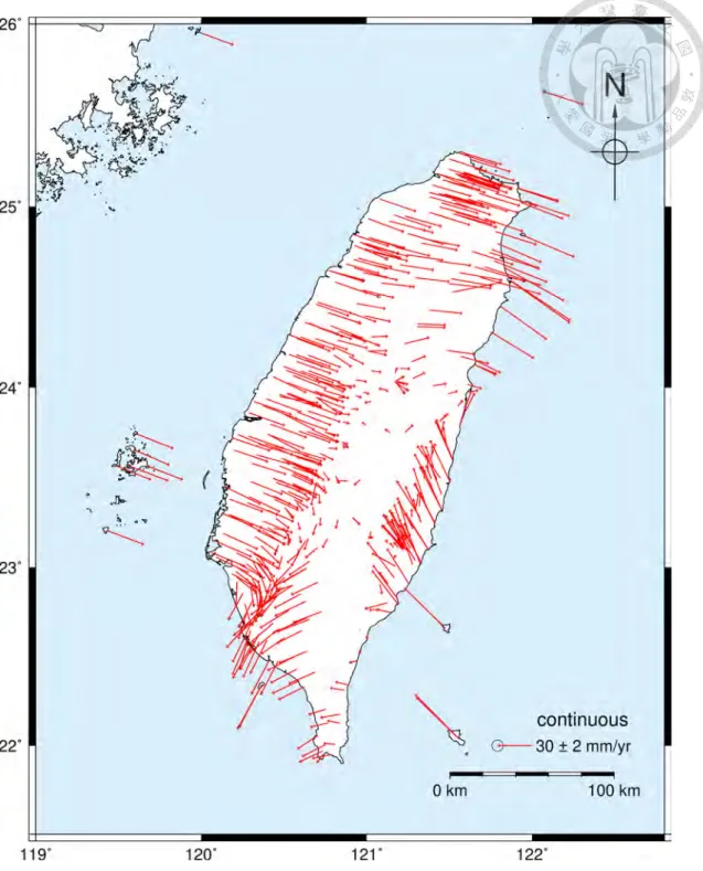
The continuous GPS data from 1993 to 2017 used in this study was processed by GPS lab at the Institute of Earth Sciences, Academia Sinica (http://gps.earth.sinica.edu.tw). Figure 6 is the GPS stations used in this study. The calculated velocities are under the ITRF2008 (Rebischung et al., 2011), the reference frame that realizes ITRF2008 is IGS08. Since the surface velocities change rapidly in short distance across the Taiwan island, this study assumes that block movements in this region are nearly horizontal and neglects the impact of Euler vector in a way to directly use north and east velocities to stands for block movements of the Earth. Figure 7 demonstrates the horizontal GPS velocity fields in Taiwan.
Figure 6 The 492 continuous GPS stations used in this research.
Figure 7 The horizontal GPS velocity fields of Taiwan, relative to IGS08.
In order to get the meaningful partition of the GPS dataset, this study uses three statistical methods including the elbow method, average silhouette method and gap statistic method to determine the optimal k for clusters. The gap statistic method ran the Monte Carlo simulation 2000 times to get the optimal k. Detailed k value can refer to Appendix 1. The result of the elbow method and average silhouette method are showing the optimal k is 4. Follow this result, we can divide the velocity filed into four major groups (Figure 8).
Figure 8 GPS velocity fields for Taiwan. The left one is the original version and the right one is the velocity field which is separated by cluster algorithm. Different colors mean different blocks in Taiwan, the green cluster means the Coastal Range, the blue cluster means the Pingtung Plain, the orange cluster means the Western Foothills and the purple cluster means the Eurasian continental margin.
These four groups can refer to different tectonic implications on a large scale.
However, according to the result of the geological survey and the geodetic measurements (Shyu, 2005; Ching et al., 2011c; Chang et al., 2016; Shyu et al., 2016), we can confirm that the tectonic settings of Taiwan are more complicated than the four blocks.
In addition to the statistical methods, this study estimates the optimal number of blocks based on geographic distribution. The statistical methods only consider the characteristics of data and clusters in the velocity space. With increasing the number of clusters, we can still separate more clusters until the localities of the velocities in the same cluster start to be distributed geographically. In other words, this study also examined the number of clusters based on the cluster distributions in the geographic space. In this case, we assumed that the clustering no longer has geographic meaning and then stopped the clustering process. In the process of clustering, some boundaries of blocks can fit the known active structures very well but some of them cannot. 0 will discuss the tectonic implications of these blocks.
4.1 Pre-process Tests
Before doing the cluster analysis, I did some simple pre-process tests to examine the robustness of the K-medoids clustering for the GPS velocities. This section focuses on the influence of the reference frame of the GPS velocities and the distribution condition of GPS stations. The former one is considering the input velocity fields of GPS data and the latter one is taking account of the uneven distribution of GPS stations. The clustering algorithm will choose the initial data points randomly as the means or medoids to do the iterative calculation, however, it is uncertain that the result will not change whether the distribution of GPS stations even or not. Therefore, this part uses some simple pre-process tests to examine these impact factors.
4.1.1 Reference frame
The International Terrestrial Reference Frame (ITRF), proposed by The International Earth Rotation and Reference Systems Service (IERS) is designed to define the GPS coordinates and the motions of GPS stations through analyzing the geodetic data collected from geodetic measurements including GPS, Very-long-baseline Interferometry (VLBI), Satellite Laser Ranging (SLR), and Doppler Orbitography and Radio-positioning Integrated by Satellite (DORIS). The reference frame can provide a basis for the calculation of the position of measurements and useful to analyze the motions of tectonics.
Since the shape of Earth’s surface is constantly changing with time, to maintain the accuracy, the reference frame needs to be updated every few years and it will be labeled by the year. For example, the version of the reference frame in this study is IGS08, which is based on the ITRF2008 and maintained by the International GNSS Service (IGS).
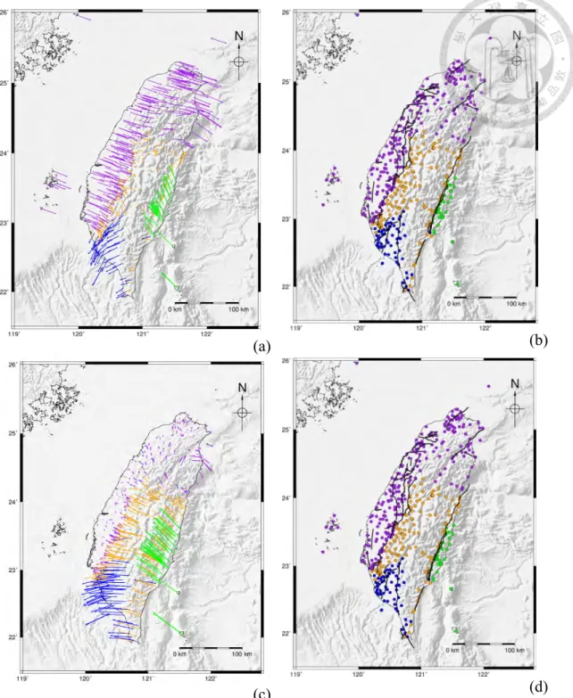
The reference frame can provide many views to observe the relative movements of the tectonics. Since one can refer GPS velocities to different reference points, the GPS velocity field will reflect different patterns. In Figure 9, both of two colors are the velocity fields in Taiwan and each color means relative to one reference frame. The blue one is relative to the ITRF reference frame and the green one is relative to the S01R station, which is a common reference point located in the stable Asian continent margin.
Furthermore, the velocity patterns are accordingly different (Figure 10a, Figure 10c).
To examine if the difference can influence the result of clustering or not, this study cluster these two sets of velocity fields based on the statistical methods described in section 3.3. Although they have different velocity patterns, the result after clustering is still the same (Figure 10b, Figure 10d). Simpson et al. (2012) examined this question as well and the result shows that no matter the data was referred to fixed North America, fixed Pacific, or fixed Sierra Nevada-Great Valley plates, the clusters are very similar.
This test suggests that as long as the patterns of relative distribution are the same, it will not influence the result of clustering.
Figure 9 Velocity fields relative to ITRF and S01R reference frames. The blue one is relative to the ITRF reference frame and the green one is relative to the S01R station.
(a) (b)
(c) (d)
Figure 10 Clustering result of different reference frames. Different color means different groups. (a) is the GPS velocity field relative to ITRF which presented as an arrow, (b) is the result of Figure 10a after cluster which presented as point, (c) is the GPS velocity field relative to S01R which presented as an arrow, and (d) is the result of Figure 10c after cluster which presented as point. The same color represents the same group
4.1.2 Velocity Distribution
Limited by various factors, such as topography and land uses, the distribution of GPS stations is usually spatially not uniform. It is uncertain whether this uneven distribution will affect the clustering result or not. In order to assess the impact of the distribution, this study sets up a simple 10 by 10 grid with a different value of velocity (Figure 11), which simulates situations of different distributions of the GPS stations. As explained above, in reality, the distribution is not always even and it needs to examine how the distribution affects the clustering results. For example, if the number of stations with high velocities is more than the number of stations with low velocities, the boundary between the two blocks may be shifted. This study selects several stations randomly and runs the cluster analysis. The result shows that no matter how many stations are selected or how the distribution of these stations are, basically there is the clustering results remain stable (Figure 12).
By examining these factors, which could influence the result of clustering, the synthetic tests confirmed that the reference frame and the distribution of stations do not have a significant effect on the result. Moreover, cluster analysis indeed can offer some information to detect the blocks in which velocity or characteristic is not similar to others.
Figure 11 Velocity setting of the synthetic data which is 10 by 10 grid. The left one means the velocity of each blocks and the right one means different groups. The velocity of the stations in the green block is 10, in the pink block is 20, in the orange block is 30, and in the purple block is 40.
Figure 12 The result after random selection. The value at the lower-left means the numbers of the station which chooses in this test.
4.2 Threshold for Stopping
According to several statistic methods to evaluate, we can get the optimal number with statistical meaning. However, this number only reflects the blocks on a large scale rather than actual blocks bounded by active structures. Therefore, this study continues to process the clustering with different values of k until the distributions of velocities in the same cluster have no geographical meaning. When the number of clusters is increasing, the number of velocities in the same cluster may decrease so such clusters with few data points may be not representative, or the GPS stations that belong to the same group but may be far away from each other in the geographic space. Therefore, although the velocities have similar values to be classified into the same cluster, no neighboring relationship implies that they are not in the same tectonic block. That is the criterion for stopping clustering in this study.
Chapter 5 Result
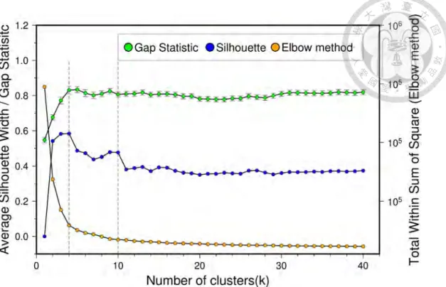
In this chapter, the results of the K-medoids are presented to separate Taiwan into k domains. The optimal number is four based on the statistic results including the elbow method, the average silhouette method, and the gap statistic method (Figure 13). In addition, there is also a significant turn when ten in the result of the silhouette test. This chapter will demonstrate the clustering result when k = 4 and 10 for the whole Taiwan first. After that, I cluster the GPS for each domain which separate accordingly the geographical characteristics and discusses the area clustering result.
Figure 13 Statistic results for Taiwan. The orange line is the result of the elbow method, the blue line is the result of the average silhouette method, and the green line is the gap statistic result. The dashed line is the significant turning point which indicates the optimal number for the clustering result.
5.1 Taiwan
5.1.1 4 clusters
According to the statistic result (Figure 13), Taiwan can be divided into four domains which separated by the three boundaries including the Longitudinal Valley, the Western Foothills and the Eurasian continental shelf, which represents different tectonic movements across the suture of arc-continent collision, the deformation front, and southwestward movement of Pingtung Plain possibly associated with tectonic extrusion (Figure 14).
Figure 14 Clustering result for whole Taiwan when k = 4.
5.1.2 10 clusters
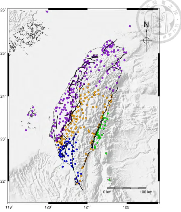
When k = 10, there are some obviously cluster including the Taipei basin and the Western Foothills (purple dots), Ilan plain (yellow dots), east of the Longitudinal Valley fault (light green dots), west of the Longitudinal Valley fault (brown dots), north section of the Central Range (cyan dots), clusters along the Western Foothills (red dots), south
section of the Central Range (pink dots), Chuchiungkeng-Muchiliao fault and Chungchou fault (orange dots), clusters between the Kaoping River structure and the Chaochou structure (blue dots), and west of the Fengshan structure (salmon pink dots).
Figure 15 Clustering result for whole Taiwan when k = 10.
5.2 Local area
To reduce the effect of the outlier and make the clustering result can be close to the real world, I tried to do the cluster analysis for local GPS stations rather than GPS stations in whole Taiwan and separated Taiwan into four domains according to the geographical characteristic, including the (I) northern Taiwan, (II) western Taiwan, (III) eastern Taiwan, and (IV) southwestern Taiwan (Figure 16). Table 1 is the number of GPS stations in each domain. After grouped thee GPS stations, I use the same statistic methods to determine the optimal number for each domain. This section is divided into four subsections, each of which presents the clustering result for each domain.
Table 1 GPS stations in each domain.
Northern Western Eastern Southwestern
Stations 85 168 132 107
Figure 16 Four domains in Taiwan. I: Northern Taiwan; II: Western Taiwan; III:
Southwestern of Taiwan; IV: Eastern Taiwan. The black line is the active structures announced by the CGS and TEM.
5.2.1 Northern Taiwan
The statistic result shows that there is not an obvious velocity change in northern Taiwan (Figure 17). The elbow method indicates that no matter what the number of clusters, the within-cluster sum of the square in northern Taiwan is very small. Even the result of the gap statistic method or the average silhouette method, the optimal number of clusters is low. Figure 18 and Figure 19 shows the clustering result of the gap statistic and the average silhouette, respectively. Due to the insignificant velocity change, it is difficult to identify the clusters in northern Taiwan. The Shanchiao fault is the principal fault of northern Taiwan, however, the slip rate of the Shanchiao fault is low and it has the inconspicuous velocity change (Shyu et al., 2005b; Shyu et al., 2016) that make it is hard to be identified. The Taoyuan and Hsinchu areas are at the transition between the waning collision and the post-collision collapse (Shyu et al., 2005b) and they can be separated from the Taipei Basin in the result of average silhouette method (Figure 19).
Figure 17 Statistic result for Northern Taiwan. The dash line at k = 1 and 2 is the optimal number of blocks which calculated by the gap statistic method and average silhouette method, respectively.
Figure 18 The clustering result of northern Taiwan by the gap statistic method.
Figure 19 The clustering result of northern Taiwan by the average silhouette method.
5.2.2 Western Taiwan
There are three subparallel faults including the Changhua fault, the Chelungpu fault, and the Tamaopu-Shuangtang fault, from west to east in western Taiwan. These structures are merged at the southern Taichung domain (Shyu et al., 2005b). The statistic result shows that western Taiwan can be divided into two or three domains (Figure 20). Figure 21 and Figure 22 demonstrate similar patterns that coincide with the locations of the active faults in western Taiwan. Whether the number of clusters is two or three, the Chelungpu fault can be identified in both results.
Figure 20 Statistic result for Western Taiwan. The dash line at k = 2 and 3 is the optimal number of blocks which calculated by the gap statistic method and average silhouette method, respectively.
Figure 21 The clustering result of western Taiwan by the gap statistic method.
Figure 22 The clustering result of western Taiwan by the average silhouette method.
5.2.3 Eastern Taiwan
In eastern Taiwan, both of the gap statistic method and the average silhouette method indicate that the number of clusters in eastern Taiwan is three (Figure 23), including the
Ilan Plain (green dots), the east of the Longitudinal Valley fault (orange dots) and the west of the Longitudinal Valley fault (blue dots) (Figure 24 and Figure 25). Due to the back- arc extension of the Okinawa Trough, the Ilan Plain is rapidly sinking and bounded by the two normal fault systems, which can be identified from geomorphic expression (Shyu et al., 2005b). Other than that, affected by the obvious velocity discrepancy, the Longitudinal Valley fault is identified as the boundary in the clustering result and divided the GPS stations into the west section and the east section.
Figure 23 Statistic result for Eastern Taiwan. The dash line at k = 3 is the optimal number of blocks which calculated by the gap statistic method and average silhouette method.
Figure 24 The clustering result of eastern Taiwan by the gap statistic method.
Figure 25 The clustering result of eastern Taiwan by the average silhouette method.
5.2.1 Southwestern Taiwan
In southwestern Taiwan, the statistical methods show two different results (Figure 26), in the gap statistic method, there are only two groups in southwestern Taiwan and bounded by the Chishan fault (Figure 27), however, according to the average silhouette method, the GPS stations can be divided into seven groups (Figure 28). The Hsinhua fault, the Chungchou fault, the Hsiaokangshan fault, the Fengshan fault, and the Chaochou fault can be identified when southwestern Taiwan be separated into seven groups.
Figure 26 Statistic result for Southwestern Taiwan. The dash line at k = 2 and 7 is the optimal number of blocks which calculated by the gap statistic method and average silhouette method, respectively.
Figure 27 The clustering result of southwestern Taiwan by the gap statistic method.
Figure 28 The clustering result of southwestern Taiwan by the average silhouette method.