時域全波電磁模擬的模型降階與遲時響應

國立臺灣大學電機資訊學院電信工程學研究所 博士論文

Graduate Institute of Communication Engineering College of Electrical Engineering and Computer Science

National Taiwan University Doctoral Dissertation

時域全波電磁模擬的模型降階與遲時響應 Model Order Reduction and Late-Time Responses of Time-Domain Full-Wave Electromagnetic Simulations

黃定彝 Huang, Ting-Yi

指導教授：吳瑞北 博士 Advisor: Wu, Ruey-Beei, Ph.D.

中華民國九十七年七月 July, 2008

黃定彝撰

97 7

時域全波 電磁模 擬 的模型降 階與遲 時 響應

究所

黃定彝撰

97 7

時域全波 電磁模 擬 的模型降 階與遲 時 響應

究所

摘要

本論文提出於時域電磁全波模擬過程中輔以 Krylov 子空間模型

降階的混合型方法，有效率地求得封閉系統的遲時響應。在本論文

提出的混合型方法中，模型降階程序通常於激發源消失之後啟動，

負責萃取出系統主要且活躍的模態，並利用這些模態的線性組合建

構系統的遲時響應。由於有效利用在空間上得到的資訊，在訊源消

失並於系統中往返之後，此方法只需要少數額外的時域迭代就能夠

得到足夠數量的激發模態。適當地萃取出系統的主要模態之後，便

可以輕易地用解析公式重建系統的遲時響應。利用本論文中提出的

技巧來實現這類型的混合方法，現存的時域模擬程式碼將得以重覆

使用。論文之中亦提供數個數值模擬範例以供檢驗此類方法的正確

性、效率、收斂性以及複雜度。由這些範例中皆可以觀察到模型降

階程序只需運作少量步驟，混合方法便能得到與直接進行時域計算

相當一致的結果。

Abstract

Hybrid methods combining time-domain full-wave electromagnetic simulation and Krylov subspace based model order reduction techniques are proposed for efficiently obtaining the late-time responses of closed systems. In general, model order reduction process is applied after the sources fade to zero for extracting the active modes in the system. Late-time responses are then constructed by the linear combination of the extracted modes. Taking advantage of the space information, only few direct time domain iterations are required after the sources fade to zero with additional round-trip time before the extraction of the excited modes. After the dominant modes are properly extracted, the late time response of the system can be easily reconstructed by analytic expressions. With the proposed hybridizing techniques, existing codes of time-domain simulation can be resorted. Several numerical examples are provided for the verification of the correctness, efficiency, convergence, and complexity of the proposed hybrid methods, which show that with only very few iterations of model order reduction, good agreement can be achieved between the results of the proposed hybrid methods and those obtained from direct time-domain iterations.

i

Table of Contents

Table of Contents ... i

List of Figures... v

1 1 Introduction... 1

1.1 Research Motives... 1

1.2 Literature Survey ... 4

1.3 Contributions ... 7

1.4 Chapter Outlines ... 9

2 Theory... 13 2 2.1 Finite-Difference Time-Domain Method... 14

2.1.1 Time Marching in TDTD... 15

2.1.2 FDTD Equations in Matrix Form ... 17

2.1.3 Time-Reversal FDTD Equations ... 19

2.2 Delaunay-Vononoi Modeling of Power-Ground Planes in Time-Domain. 20 2.2.1 Delaunay-Vononoi Modeling of Power-Ground Planes ... 23

ii

2.2.2 Time Marching Scheme for Delaunay-Vononoi Modeling of

Power-Ground Planes ...26

2.3 Model Order Reduction with Krylov Subspace Methods ...28

2.3.1 Krylov Subspaces ...29

2.3.2 Lanczos Algorithm ...30

33 Late-Time Response by FDTD Method and Lanczos Algorithm...33

3.1 Hybridizing FDTD and Lanczos Algorithm by Time-Reversal technique.34 3.2 Homogeneous PEC Cavity ...42

3.2.1 Simulation Settings...42

3.2.2 Late-Time Responses...44

3.2.3 Modal Patterns...47

3.3 Inhomogeneous PEC Cavity...47

3.3.1 Simulation Settings...47

3.3.2 Late-Time Responses...49

3.3.3 Modal Patterns...53

iii

3.4 Convergence and Complexity... 53

3.4.1 Convergence ... 54

3.4.2 Complexity... 56

3.5 Summary of the Chapter ... 59

4 4 Late-Time Response for Delaunay-Vononoi Modeling of Power-Ground Planes in Time-Domain with Krylov Subspace Method... 61

4.1 Krylov Subspace Method for Delaunay-Vononoi Modeling of Power-Ground Planes in Time-Domain... 62

4.2 Power-Ground Plane of Simple Geometry ... 68

4.2.1 Geometry ... 68

4.2.2 Simulation Results ... 70

4.2.3 Modal Patterns ... 73

4.3 A More Realistic Power-Ground Plane... 76

4.3.1 Geometry ... 76

4.3.2 Simulation Results ... 79

4.3.3 Modal Patterns ... 82

iv

4.4 Convergence and Complexity ...84

4.4.1 Convergence ...84

4.4.2 Complexity ...90

4.5 Summary of the Chapter...93

5 5 Conclusions ...95

5.1 Summary of the Work...96

5.2 Suggestions for Future Work ...97

References ...101

Publication List of Ting-Yi Huang ...107

A. Journal Papers...107

B. Conference Papers ...109

v

List of Figures

Fig. 2.1 Yee’s cell [1] for descretization of Maxwell equation for the finite-difference time-domain method in three-dimension. ... 14

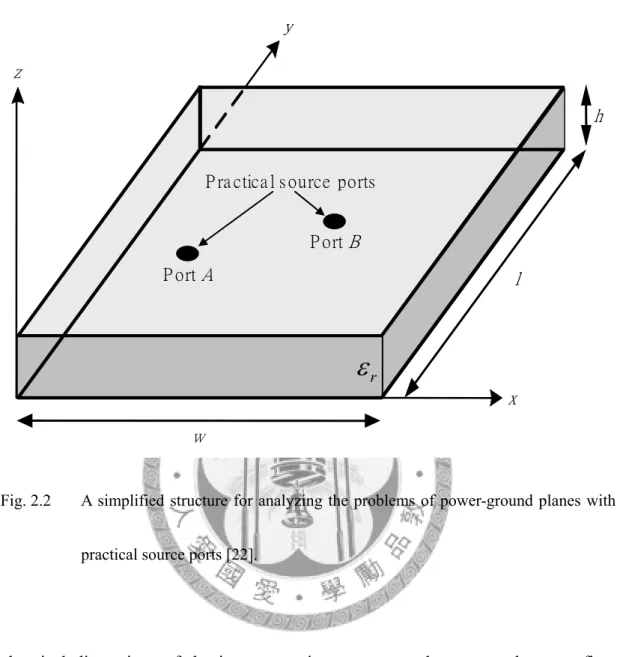
Fig. 2.2 A simplified structure for analyzing the problems of power-ground planes with practical source ports [22]. ... 21

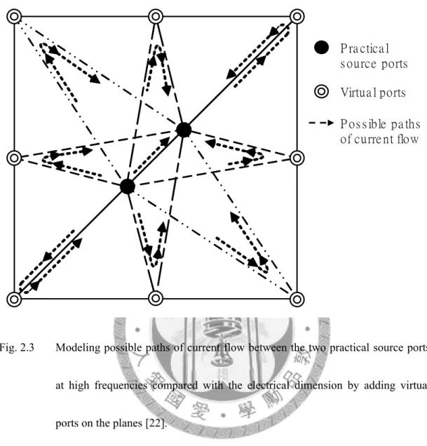
Fig. 2.3 Modeling possible paths of current flow between the two practical source ports at high frequencies compared with the electrical dimension by adding virtual ports on the planes [22]. ... 22

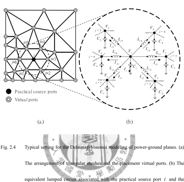
Fig. 2.4 Typical setting for the Delaunay-Vononoi modeling of power-ground planes. (a) The arrangement of triangular meshes and the placement virtual ports. (b) The equivalent lumped circuit associated with the practical source port

i and the virtual ports connected. ... 23

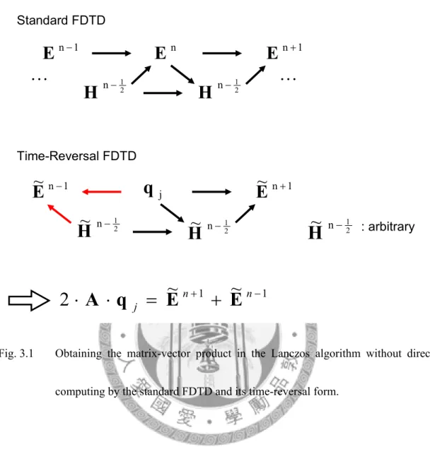
Fig. 3.1 Obtaining the matrix-vector product in the Lanczos algorithm without direct computing by the standard FDTD and its time-reversal form.... 37

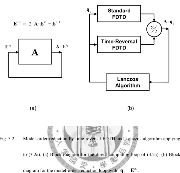
Fig. 3.2 Model-order reduction by time-reversal FDTD and Lanczos algorithm

vi

applying to (3.2a). (a) Block diagram for the direct computing loop of (3.2a). (b) Block diagram for the model-order reduction loop with

1

E

q

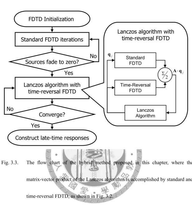
Fig. 3.3. The flow chart of the hybrid method proposed in this chapter, where the matrix-vector product of the Lanczos algorithm is accomplished by standard and time-reversal FDTD, as shown in Fig. 3.2. ...41

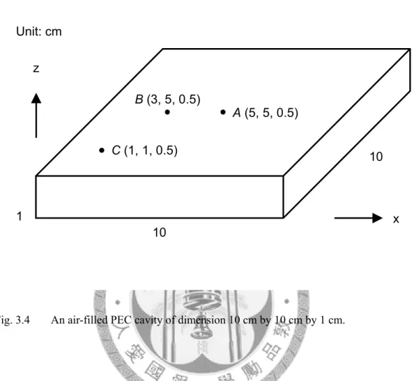
Fig. 3.4 An air-filled PEC cavity of dimension 10 cm by 10 cm by 1 cm...43

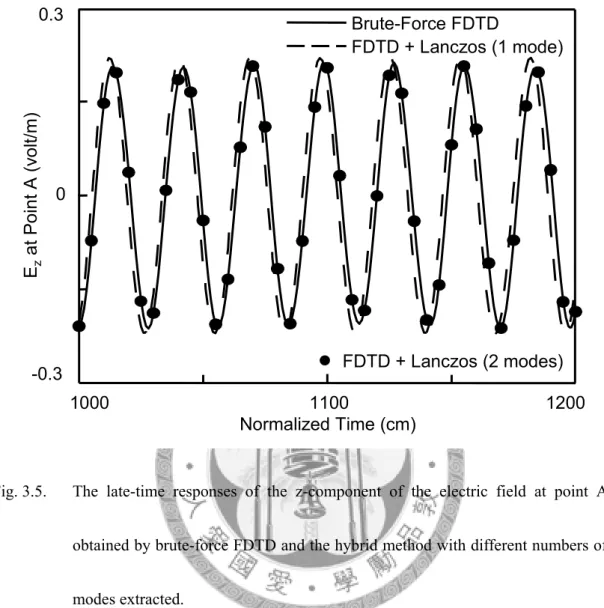
Fig. 3.5. The late-time responses of the z-component of the electric field at point A obtained by brute-force FDTD and the hybrid method with different numbers of modes extracted...44

Fig. 3.6. The late-time responses of the z-component of the electric field at points B and C obtained by brute-force FDTD and the hybrid method with two modes extracted...45

Fig. 3.7. Modal patterns of the first two modes extracted by Lanczos algorithm.

(a) The first mode extracted; (b) the second mode extracted. ...46

Fig. 3.8. An air-filed PEC cavity with a dielectric object...48

vii

Fig. 3.9. The late-time responses of (a) the y-component at the point (0.5 , 10 , 10)(mm) and (b) the x-component at the point (15 , 0.5 , 10 )(mm) of the magnetic field in Fig. 3.5 which is excited by a Gaussian pulse with a longer rise time... 50

Fig. 3.10. The late-time responses of the y-component of the magnetic field at the point (0.5 mm, 10 mm, 10 mm) in Fig. 4 which is excited by a Gaussian pulse with a shorter rise time. ... 51

Fig. 3.9. Modal patterns of the magnetic field at the z=10mm plane in the structure shown in Fig. 3.8 for the first six modes extracted by Lanczos algorithm... 52

Fig. 3.12. The absolute value of the smallest expansion coefficient a_min normalized to the largest one,

a

Fig. 3.13. The magnitude of the frequency response of the magnetic field obtained at the point (0.5 mm, 10 mm, 10 mm) in Fig. 4 in the second example in IV with a high frequency excitation... 58

viii

Fig. 4.1. Constructing a Krylov subspace for the approximation of system matrix

A directly from a series of system response in time...63

Fig. 4.2. Flow chart of the hybrid method proposed in this chapter, where the Krylov subspace is constructed directly from the pre-stored voltage vectors as shown in Fig. 4.1. ...66

Fig. 4.3. The geometry of a 50mm×50mm×1.6mm power-ground plane with an excitation port at (20mm, 30mm). (a) Three-dimensional view. (b) Top view...69

Fig. 4.4. Mesh setting for the simulation of the structure shown in Fig. 4.3. (a) Locations of the input port (solid dot) and virtual ports (double circle).

(b) Arrangement of the triangular meshes on the plane...70

Fig. 4.5. Late-time responses obtained by direct time-domain iteration (solid line) and hybrid method (dashed line) for the structure with a geometry shown in Fig. 4.3 and a mesh settings in Fig. 4.4...71

Fig. 4.6. The frequency responses of the input impedance at the port of Fig. 4.3 obtained by direct inversing the Y-matrix in frequency domain (solid

ix

line) and the frequency transform by FFT of the late-time responses obtained by direct time-domain iteration (dashed line) and the hybrid method (dotted line)... 72

Fig. 4.7 Frequency responses and modal patterns obtained by (4.9) for the cavity shown in Fig. 4.3 with (a) m=1, n=0 (b) m=0, n=1, and (c) m=1, n=1, respectively. ... 74

Fig. 4.8. Modal patterns of (a) the first mode and (b) the second mode extracted by the hybrid method for the structure shown in Fig. 4.3 with mesh settings shown in Fig. 4.4. ... 75

Fig. 4.9. A more realistic power-ground plane with a clipped corner and an aperture on the top metal. (a) The geometric parameters of the power-ground plane. (b) The mesh setting for simulation... 77

Fig. 4.10. (a) The time response of a standard Gaussian pulse and (b) its frequency response; and (c) the time response of a modulated Gaussian pulse with zero DC level and (d) its frequency response. ... 78

Fig. 4.11. The magnitude of the frequency responses of the input impedance at the

x

port shown in Fig. 4.9. The solid line is obtained by direct inversing the Y-matrix in frequency domain. The dashed and dash-dotted lines are the results by time-domain iteration and FFT with two different sources of excitation. ...80

Fig. 4.12. The magnitude of the frequency responses of the input impedance at the port shown in Fig. 4.9 obtained by direct time-domain iteration (solid line) and the hybrid method (dashed line) with FFT. ...81

Fig. 4.13. (a) The first mode and (b) the second mode of the structure shown in Fig. 4.9, which are extracted by the hybrid method; and (c) the first mode and (b) the second mode of the same structure extracted by Ansoft^® HFSS^™. ...83

Fig. 4.14. (a) Mesh1, a coarse mesh setting, (b) Mesh2, a marginal mesh setting, and (c) Mesh3, a fine mesh setting arranged for the verification of self convergence of the hybrid method proposed in this chapter. ...87

Fig. 4.15. Frequency responses of the input impedances at the incident port denoted by black dots in Fig 4.13 for mesh settings Mesh1 (dotted line), Mesh 2 (dashed line), and Mesh3 (solid line). ...88

xi

Fig. 4.16. Modal patterns extracted by the hybrid method. (a) The first mode and (b) the second mode extracted from Mesh1; and (c) The first mode and (d) the second mode extracted from Mesh2... 89

1

1 1

Introduction

IME-domain full-wave electromagnetic simulations have been widely used in modern digital and analog circuit design. This thesis proposes a model-order reduction technique for the late-time responses of time-domain full-wave electromagnetic simulation. As an introduction, the research motives of this work will be discussed first in this chapter. Literature survey of related works is then presented, followed by the major contribution of this work. Outlines of each chapter will also be briefly described in the end of this chapter.

1.1 Research Motives

Modern electronic circuits are often composed of digital and analog hybridization. As the fabrication processes such as very large scale integrated (VLSI) circuit and low-temperature co-fire ceramic (LTCC) advance, the complexity and

T

circuit size has grown to an extraordinary level. Operation speed and frequency range of the signal also increases rapidly as computer and communication applications mature. Circuit level simulation no longer satisfies the precision desire for some critical parts or even the whole circuits at design stage. On the other hand, full-wave electromagnetic simulation provides accurate results with the expenses of time and memory requirement of computation. Typical design procedure has then become extracting the characteristics such as scattering coefficients or impedance matrices of the critical parts, and then the extracted “black boxes” become new circuit components in the circuit level simulation. Therefore time-domain full-wave methods are often preferred in package level co-simulation, especially when dealing with cases where non-linear components are presented, due to their easy integration with existing commercial circuit simulation software packages, e.g. SPICE.

The finite-difference time-domain (FDTD) method [1], [2] is well known for its simple implementation and high efficiency in solving various general-purpose problems. In general, sources such as Gaussian pulses or time-domain reflectometry (TDR) signals are injected into the areas of interest and a few field points wherein are often chosen to be observed. The FDTD solvers update all the field points in the

areas continually as time marching until the injected energies decay to a certain level.

The relation between observing field points and injecting sources are then set up to find the characteristics such as transfer functions or scattering parameters of the system. However, this strategy fails in most low-loss close problems and some open problems with high-Q materials. The energies decay very slowly or may even remain at a nonconverging level permanently in certain cases.

Steady-state responses are often desired for finding the system characteristics in the frequency domain. In order to increase the resolution in the frequency domain, a steady-state response in a long enough time interval is needed to be calculated. For complex structures, fine meshes are often required to improve accuracy and, consequently, the time step in conventional FDTD simulation should also be small enough to satisfy the stability condition. It is a time-consuming task to obtain the frequency-domain characteristics under such conditions. In addition, only a few field points need to be taken into consideration in most practical applications while fields at all points in the computational domain should be calculated at each time iteration.

How to efficiently get the steady-state response at those field points concerned therefore becomes an important subject. [3]

1.2 Literature Survey

Techniques commonly used for the extrapolation of late-time responses in FDTD simulations are Prony’s methods [2], [4]-[8]. It is a technique for modeling sampled data as a linear combination of complex exponentials, therefore particularly suitable for calculating the resonant frequency and Q of a resonating structure [2].

With data sampled at a relatively small number of time iterations, the late-time responses can be effectively predicted [6]. However, temporal data are needed to be sampled at a sufficient number of locations, or the frequency-domain circuit parameters will not be accurate [8].

Another way to retrieve the spectral-domain data from timedomain simulators are the filter-diagonalization methods [2], [9]-[13]. This technique recasts the problem of spectral analysis of a short segment of a time-dependent signal into an eigenvalue problem [2]. These methods are useful in extracting the mode frequencies and decay constants of high-Q cavities [12]. With properly chosen basis sets, the spectral parameters obtained by the filter-diagonalization method can be used to construct a high resolution Fourier spectrum, circumventing the Fourier uncertainty

principle [13]. Therefore, cases of nearly degenerate modes can be effectively handled.

The aforementioned techniques usually deal with data sampled in a long period of time at few points. Increasing the sample temporal points can improve the accuracy, but with larger computational overhead as a tradeoff. On the other hand, it can be advantageous to exploit the space information that is necessary to be updated at each FDTD iteration. Model-order reduction techniques combining with the FDTD that recently arose are the Lanczos algorithms [14], [15]. Taking advantages of the sparsity of the equivalent matrix of the FDTD operator, although still large in size, the model order can be efficiently reduced since the Lanczos algorithm is able to convert a large sparse matrix into a much smaller tridiagonal matrix with very low overheads. The eigenvalues of the reduced matrix are approximately equal to some of the extremal eigenvalues of the original matrix. The associated eigenvectors of the original matrix can also be recovered from the eigenvectors of the reduced matrix through a simple transformation.

Several papers have been proposed for dealing with the model-order reduction of the FDTD method by the Lanczos algorithm. A modified Lanczos algorithm is

proposed for the computation of transient electromagnetic fields [16]. Accurate representation of the transient electromagnetic fields is obtained on a certain bounded interval in time. However, this is not suitable for obtaining the steady-state response for practical problems since more Lanczos iterations may be required in order to increase the time interval of accurate simulation. Tradeoffs between divergence owing to loss of orthogonality and slow convergence due to re-orthonormaliztion will arise as Lanczos iterations increase [15].

Rapid FDTD simulation without time stepping is also proposed [17]. With the reduced-order model extracted by the Lanczos algorithm, the response can be obtained at any frequency. However, the number of FDTD update equations is doubled. The original system and its adjoint problem are both needed because the asymmetric Lanczos algorithm is applied [18].

This work provides a different approach in combining the FDTD method and Lanczos algorithm based on [19]. The basic theory is detailed in Chapter 2 and the hybrid method as well as some numerical examples in provided in Chapter 3. With the Lanczos algorithm, modes for a source-free FDTD operator concerning either electric or magnetic fields only are extracted. Utilizing the time-reversal property of

the FDTD [20], the existing FDTD codes can be resorted to directly.

For the analysis of power-ground plane issues in high-speed digital circuit systems, an efficient model of power-ground planes based on the concept of model network has been proposed [21], [22]. A novel model consisting of the virtual ports and triangular meshes with the distributed lumped circuit elements is established, which has the advantages of constructing the SPICE-compatible models to facilitate the multi-layer design analysis for power-ground planes. With little modifications, a time marching scheme similar to FDTD based on this method can be combined with Krylov subspace methods

1.3 Contributions

As mentioned in the previous section, this work provides a novel approach combining the FDTD method and Lanczos algorithm. Unlike other approaches which take time information over few space samples into consideration, the proposed hybrid method utilizes the space information which is automatically evaluated every time step in FDTD. Since the most time consuming bottleneck is FDTD iteration itself, less iterations needed for completing a model order reduction process is

preferred.

Taking advantages of the space information, Lanczos algorithm extracts dominant modes rapidly. This means only few FDTD iterations are needed for the proposed hybrid method to converge. The modal information is then used to construct the late-time response of the system. Only the responses at those points concerned is computed with nearly constant order of complexity. After introducing time-reversal FDTD into the hybrid method, with little modification, existing FDTD code are also preserved.

Another hybrid method dealing with time-domain model order reduction for analyzing the power-ground planes of high-speed digital circuit systems is also proposed in this thesis. Based on the efficient model of power-ground planes presented in [22], a time marching scheme similar to FDTD is constructed. Krylov subspace method is then applied to extract the dominant mode according to the space information computed at each time step. After the modal information has been extracted, the late-time responses of the system at those points concerned are also easily determined with nearly constant order of complexity.

Unlike the FDTD/Lanczos hybrid method, time-reversal scheme is not available

for the time-domain method utilized in this hybrid method. The Krylov subspace is instead constructed from a series of space information which are stored at different time steps. With additional memory overhead, the existing codes of the time-domain method can also be preserved.

Several examples are provided for both hybrid methods, ranging from simple demonstration cases to more realistic applications. In addition to the presented simulation results for the examples, the convergence and complexity for both methods are further discussed also with a few simulation results to verify the robustness and effectiveness of the proposed methods.

1.4 Chapter Outlines

In order to provide a systematic and structured presentation of this work, the remaining contents of the thesis are organized as follows.

The basic theory which both hybrid methods based on will be described in Chapter 2. A brief review of the finite-difference time-domain method will be presented firstly, including the traditional iterative FDTD equations and its matrix form, equations involving both the electric and magnetic fields, as well as those with

single field only. Time-reversal technique for FDTD will also be described. The time-domain method based on Delaunay-Vononoi modeling of power-ground planes will then discussed, which shows how a time marching scheme similar to FDTD can be established from the efficient power-ground plane model. The last part of chapter 2 shows the key component of both hybrid methods, i.e., model order reduction with Krylov subspace methods. With these methods modes of systems can be extracted effectively for the reconstruction of late-time responses.

Chapter 3 presents the first hybrid method which efficiently evaluates the late-time response by combining finite-difference time-domain method and Lanczos algorithm. Technique that hybridizing FDTD and Lanczos Algorithm by introducing time-reversal FDTD equations is firstly described, followed by numerical examples with a homogeneous PEC cavity and an inhomogeneous PEC cavity with different excitations. Convergence and complexity is then discussed with verification from the simulation results.

The other hybrid method that reconstructs the late-time response for Delaunay-Vononoi modeling of power-ground planes in time-domain with Krylov subspace method is presented in Chapter 4. After describing the hybridizing

technique that applies Krylov subspace method on the Delaunay-Vononoi modeling of power-ground planes in time-domain, several examples inclusive of power-ground planes of a simple geometry and a more realistic power-ground plane is demonstrated.

The convergence and complexity for this method is also analyzed and verified with simulation results.

The thesis is then concluded with a summary of this work. A few suggestions for the future works will also be provided.

13

2 2

Theory

HE hybrid methods presented in this work is based on the basic theory described in this chapter. The finite-difference time-domain (FDTD) method will be briefly reviewed first. The traditional iterative FDTD equations and its matrix form, equations involving both the electric and magnetic fields and those with single field only, and time-reversal technique for FDTD will be described. Based on the Delaunay-Vononoi modeling of power-ground planes provided in [22], a time marching scheme similar to FDTD is developed. The key component of the proposed hybrid methods, model order reduction with Krylov subspace methods, with which the modes of a system are extracted effectively for the reconstruction of late-time responses, will be discussed in the last part of this chapter.

T

x

y

z

(

) (

)

(

) (

) (

)

(

)

E

E

E

H

H

Hz

Fig. 2.1 Yee’s cell [1] for descretization of Maxwell equation for the finite-difference

time-domain method in three-dimension.

2.1 Finite-Difference Time-Domain Method

The derivation of finite-difference time-domain equations in source free regions begins with source free Maxwell equations.

t E B

∂

−∂

=

×

∇ v v

(2.1a)

t H D

∂

= ∂

×

∇ v

v (2.1b)

2.1.1 Time Marching in TDTD

In source-free region with lossless isotropic media, (2.1) can be discretized with

the Yee’s cell [1] setting shown in Fig. 2.1, where the simplified coordinate notation

(

)

(

)

the space descretization Δx, Δy, and Δz, respectively. If the descretization in time is denoted as Δt with integer multiples n, the field values of the x-component of the electric field locate at ⎟

⎠

⎜ ⎞

⎝⎛ +

i

j

k

1 and time step n can be denoted as

E

2

+1 , the field values of the y-component of the magnetic field locate at ⎟

⎠

⎜ ⎞

⎝

⎛ + +

2 , 1 2, 1

j k

i

time step 2 +1

n

1 , 2, 1 + + n

k j yi

H . Notations of other field values can be

defined in a similar manner. Applying central difference method for both the differentiation in time and space, the iterative finite-difference time-domain equations can be derived as

( )

⎥⎥

⎥

⎦

⎤

⎢⎢

⎢

⎣

⎡

Δ

− Δ −

Δ −

− ⋅

= ^{+ + + + + +}

+ +

− + + +

+

+ z

E E

y E t E

H H

n k j y i n

k j y i n

k j zi n

k j zi

k j ri n

k j x i n

k j xi

2, , 1 1 2, , 1 2 , 1 2 ,

, 1 1 ,

2 , 1 2 , 1 2

1

2 , 1 2 , 1 2 0

1

2 , 1 2 , 1 0

c η μ

η

(2.2a1)

( )

⎥⎥

⎥

⎦

⎤

⎢⎢

⎢

⎣

⎡

Δ

− Δ −

Δ −

− ⋅

= ^{+ + + + + +}

+ +

− + + +

+

+ x

E E

z E t E

H H

n k j y i n

k j y i n

k j zi n

k j x i

k j ri n

k j y i n

k j

y i 2

, 1 2 ,

, 1 , 1 ,

2, 1 1

, 2, 1

2 , 1 2, 1 2

1

2 , 1 2, 1 2 0

1

2 , 1 2, 1 0

c η μ

η

(2.2a2)

( )

⎥⎥

⎥

⎦

⎤

⎢⎢

⎢

⎣

⎡

Δ

− Δ −

Δ −

− ⋅

= ^{+ + + + + +}

+ +

− + + +

+

+ y

E E

x E t E

H H

n k j x i n

k j xi n

k j yi n

k j yi

k j ri n

k j zi n

k j zi

, 2, , 1

1 2, , 1

2 , 1 2,

, 1 1

2, , 1 2 1 2

1

2, , 1 2 1 2 0

1

2, , 1 2 1 0

c η μ

η

(2.2a3)

( )

⎥⎥

⎥⎥

⎦

⎤

⎢⎢

⎢⎢

⎣

⎡

Δ

− Δ −

Δ −

− ⋅

=

+

− + +

+ + +

− + +

+ + +

+ +

+ z

H H

y H t H

E E

n k j y i n

k j yi n

k j z i n

k j z i

k j ri n

k j xi n

k j xi

2 1

2 , 1 2, 1 2 0

1

2 , 1 2, 1 2 0

1

2, , 1 2 1 2 0

1

2, , 1 2 1 0

, 2, , 1

2, 1 1

, 2,

1 c η η η η

ε

(2.2b1)

( )

⎥⎥

⎥⎥

⎥

⎦

⎤

⎢⎢

⎢⎢

⎢

⎣

⎡

Δ

− Δ −

Δ −

− ⋅

=

+ +

− +

+ + +

− + +

+ + + +

+

+ x

H H

z H t H

E E

n k j zi n

k j zi n

k j x i n

k j x i

k j r i n

k j y i n

k j y i

2 1

2, , 1 2 1 2 0

1

2, , 1 2 1 2 0

1

2 , 1 2 , 1 2 0

1

2 , 1 2 , 1 0

2, , 1 2,

, 1 1

2, , 1

c η η η η

ε

(2.2b2)

( )

⎥⎥

⎥⎥

⎥

⎦

⎤

⎢⎢

⎢⎢

⎢

⎣

⎡

Δ

− Δ −

Δ −

− ⋅

=

+ +

− +

+ + +

+

− +

+ + +

+ +

+ y

H H

x H t H

E E

n k j x i n

k j x i n

k j y i n

k j y i

k j ri n

k j zi n

k j z i

2 1

2 , 1 2 , 1 2 0

1

2 , 1 2 , 1 2 0

1

2 , 1 2, 1 2 0

1

2 , 1 2, 1 0

2 , 1 2 ,

, 1 , 1

2 , 1 ,

c η η η η

ε

(2.2b3)

, where

0

0

ε

η

μ

light in free space. At time step n, the magnetic field is first updated to the next half time step by (2.2a) with the electric field at current time step and magnetic field at previous half time step; the updated magnetic field at next half time step and the electric field at current time step is used to update the electric field to the next time step by (2.2b). After updating both fields, the FDTD iteration in a time step is completed. Time step is than moved from n to n+1. Repeatedly, the desired time responses of both fields can be evaluated.

2.1.2 FDTD Equations in Matrix Form

Let

E

H

( )

n

n

H t μ D E

H

0

η

η

and

( )

1 c ^{− +}

+ = ⁿ + ⋅Δ ⋅ _r ⋅ ^T ⋅ ⁿ

n

E t ε D H

E η

where D denotes the discrete curl operator. Substitute (2.3a) and the (n-1)-th time step of (2.3b) into the n-th time step of (2.3b), the FDTD update equation in matrix

form can be written as

( )

( ) ( )

⎦

⎤

⎢⎢

⎣

⎡

⎥⎦

⎢ ⎤

⎣

⎡

⋅

⋅

⋅

⋅ Δ

⋅

−

⋅

⋅ Δ

⋅

⋅

⋅ Δ

⋅

= −

⎥⎥

⎦

⎤

⎢⎢

⎣

⎡ ⁻

−

−

−

− +

+

n n

r T r T

r

r n

n

t c t

c

t c

E H D μ D ε I

D ε

D μ I

E

H

1 1 0

2 1 1

1 1

2 1

0

η

η

where the identity matrix is denoted by I.

Eliminating the equations involving magnetic fields in (2.4) yields an update equation with electric field only.

( )

1 c

2

2 1 ^{− − −}

+ ⋅ −

⎥⎦⎤

⎢⎣⎡ − ⋅Δ ⋅ ⋅ ⋅ ⋅

⋅

= _r ^T _r ^{n n}

n

I t ε D μ D E E

E

On the other hand, an update equation with only magnetic field concerned can also be obtained.

( )

2 1

0 c

2

2 1 ^{− − − −}

+ ⋅ −

⎥⎦⎤

⎢⎣⎡ − ⋅Δ ⋅ ⋅ ⋅ ⋅

⋅

= _{r r} ^{T n n}

n

I t μ D ε D H H

H η η

η

These two matrix equations with only a single field in (2.5) play an important role in the next chapter, where Lanczos algorithm is applied to the symmetric matrix inside the bracket. With the hybridizing technique which will be detailed later, direct evaluation of (2.5) is not required. Existing code of FDTD solvers can be reused with the introducing of additional time-reversal FDTD equations.

2.1.3 Time-Reversal FDTD Equations

The time-reversal technique in FDTD method has been proposed for the numerical synthesis of a microwave structure [20]. By slightly rearranging (2.3), the update equation can be operated backward in time as

n r

n

n

H c t μ D E

H

0

η

η

and

2 1 0 1

1 − −

− = ⁿ− ⋅Δ ⋅ _r ⋅ ^T⋅ ⁿ

n

E c t ε D H

E η

The time-reversal FDTD iterations proceed in a similar manner as ordinate FDTD. At time step n, the magnetic field is first updated to the previous half time step by (2.6a) with the electric field at current time step and magnetic field at next half time step;

the updated magnetic field at previous half time step and the electric field at current time step is then used to update the electric field to the previous time step by (2.6b).

After updating both fields, another iteration begins with the time step moving from n to n−1.

For the hybrid method presented in the following chapter, the time-reversal FDTD equations will only activate after the model order reduction procedure begins.

As long as the model order reduction procedure converges rapidly, the computation overhead increased by introducing the time-reversal FDTD equation and the numerical error cumulates in the backward iteration in time [20] can be minimized.

2.2 Delaunay-Vononoi Modeling of Power-Ground Planes in Time-Domain

A simplified structure is shown in Fig. 2.2 for analyzing the problems of power-ground planes with practical source ports [22]. A pair of close-spaced power-ground planes with length l and width w are separated by a dielectric substrate with a thickness h and a relative dielectric constant

ε

Current injecting into port A may induce a power-ground bounce noise between the planes. The noise wave travels throughout the entire planes and eventually the noise will couple to port B, causing a slightly variation to the port voltage.

Fig. 2.3 shows the modeling of possible paths of current flow between the two practical source ports at high frequencies compared with the electrical dimension by adding virtual ports on the planes [22]. As the wavelength of interests approaches the

x y

z

P ra ctica l s ource ports

w

l

h

P ort

A

P ort

B

ε

Fig. 2.2 A simplified structure for analyzing the problems of power-ground planes with

practical source ports [22].

electrical dimensions of the interconnection structures, the current does not flow straightly from port A to port B but also includes the paths spreading radially outward from port A and then reflecting from the edges of power-ground planes to port B.

This phenomenon can be effectively modeled by the novel method proposed in [22]

using an equivalent lumped circuit model with virtual ports that play the role of the distributed current transition. The values of lumped circuit elements are associated

P ra ctica l s ource ports Virtua l ports P os s ible pa ths of curre nt flow

Fig. 2.3 Modeling possible paths of current flow between the two practical source ports

at high frequencies compared with the electrical dimension by adding virtual

ports on the planes [22].

with the geometry of the triangular mesh and can be obtained by employing the Delaunay triangularization for the mesh generation and applying Voronoi tesserlation at each node.

P ra ctica l s ource ports Virtua l ports

V1 1

Li Cⁱ

C1

Vi

Ii 1

Ii V₂

V5

V4

V6 V₃

C6

C5

C3

C4

C2 5

Li

6

Li

3

Li 4

Li

2

Li ⁱ³

I

2

Ii 4

Ii

6

Ii 5

Ii

=1

j j=2

=4 5 j

j=

=6

j j=3

i

=4 j

=2 1 j

j=

=5 j

=3 6 j

j=

(a ) (b)

Fig. 2.4 Typical setting for the Delaunay-Vononoi modeling of power-ground planes. (a)

The arrangement of triangular meshes and the placement virtual ports. (b) The

equivalent lumped circuit associated with the practical source port

i

virtual ports connected.

2.2.1 Delaunay-Vononoi Modeling of Power-Ground Planes

For the typical setting of Delaunay-Vononoi modeling of power-ground planes shown in Fig. 2.4, if the arrangement of triangular meshes and the placement virtual

ports is given in Fig. 2.4a, the equivalent lumped circuit associated with the practical source port i and its connecting neighbor virtual ports, which are embraced in the dashed circle, can be determined as Fig. 2.4b, assume a lossless condition. The values of the elements in the equivalent lumped circuit model can be determined by matching the terms derived from the perspective of circuit and electromagnetic theory.

Applying the Kirchhoff’s Current Law (KCL), the relation between nodal voltages and the lumped circuit elements at the i-th node in Fig. 2.4 can be obtained as

0

6 1

− = +

∑

=

j ij

j i i

i

j L

V V V

C

j ω ω

with the notations shown in Fig. 2.4b, where the nodal voltages at the i- and j-th node are denotes by

V and

V , respectively. The shunt capacitance at the i-th node is

C and

L represents the series inductance connecting the i- and j-th

On the other hand, if the thickness h in Fig. 2.2 is small enough compare to the wavelength of interest, the voltage distribution can be approximate as a function of

coordinates (x, y), the electric and magnetic field can be written as

h z y x

Ev=−V( , )) (2.8a)

and

( V x y z )

h

H

j

ωμ

respectively. Applying Ampere’s Law

∫ ^H

^{d l}

^I

∫∫ ^{j ωε E}

^{d s}

∫

∑

1 j

ji ji j

i

l

hd j

V l V

d

H ωμ

v v (2.9a)

and

i

A

h j V s d E

j ωε

ωε

∫∫

where

d is the length of the line connecting the j- and i-th node,

l is the length

between the circumcenters of the two triangles with a common edge connecting the j- and i-th node, and

A is the area of the integration loop. Detailed derivation can be

By matching the terms in (2.7) and (2.9), the values of the lumped circuit elements is then determined as

h

C_i =ε Aⁱ (2.10a)

and

ij ij

ij l

L μhd

= , (2.10b)

which shows a relation only with the geometric parameters. Therefore once the meshes for the analysis are set, these values can then be uniquely defined.

2.2.2 Time Marching Scheme for Delaunay-Vononoi Modeling of Power-Ground Planes

For the i-th node of the equivalent lumped circuit model of power-ground planes shown in Fig. 2.4b, the node voltage and the branch current can be related with the lumped circuit elements in time domain as

dt C dV

I

and

dt L dI V

V

where

V and

V is the node voltage at the i- and j-th node, respectively,

I is the

C , and

I is the current through the series

L connecting the i- and j-th node. These two current can be related by

KCL as

=0 +

∑

j ij

i

I

I

Since the current flows from the i- to j-th node in the opposite direction as from j- to

i-th node, it is obvious that I

I

Let the time in (2.11) be dicretized as n⋅Δt. If the node voltages is located at the integer multiples as

V

V

( n

t )

⎠

⎜ ⎞

⎝

⎛ ⎟⋅Δ

⎠

⎜ ⎞

⎝⎛ +

+ =

t n

I I

2

2 1

1

and

⎟⎠

⎜ ⎞

⎝

⎛ ⎟⋅Δ

⎠

⎜ ⎞

⎝⎛ +

+ =

t n

I I

2

2 1

1

, applying central difference to the differentiation in time in

(2.11)yields

2 1

1 +

+ = +Δ _iⁿ

i n i n

i

I

C V t

V

and

(

)

n i ij n ij n

ij V V

L I t

I ⁺²¹ = ⁻²¹ +Δ − . (2.12b)

(2.11c) can also be rewritten as

∑

+ =−

j n ij n

i

I

I

1 2

1

(2.12c)

with branch currents ²

1 2

1 +

+ =− ⁿ_ji

n

ij I

I . For the time marching scheme of Delaunay- Vononoi modeling of power-ground planes, the iteration at time step n begins with (2.12b), where the branch currents through the series inductances connecting the nodes are updates to the next half time step with those at previous half time step and the voltages at all nodes at current time step. The current through the shunt capacitance at each node can then be update by (2.12c). After that all node voltages can be update to the next time step with their value at current time step and the currents at next half time step. Time step is then moved from n to n+1 for the beginning of a new iteration.

2.3 Model Order Reduction with Krylov Subspace Methods

Model order reduction for linear systems is often associated with a few numbers

of the largest and/or smallest eigenvlaues and their eigenvectors. For a large sparse symmetric n×n matrix A, the approximation of its extremal eigenvalues can be efficiently extracted through a sequence of tridiagonal matrices generated by Krylov subspace methods, where the extremal eigenvalues of the tridigonal matrices are progressively better estimates of A’s extremal eigenvalues [15].

2.3.1 Krylov Subspaces

For a Rayleigh quotient defined as

( )

x

x x

x x x

r

A

, (2.13)

where A is a symmetric n×n matrix and x is a column vector with dimension n, the maximum and minimum values of r

( )

^λ

( )

^λ

( ) ^A

Define a sequence of orthonormal vectors

Q

[ q

q

q

]

M as

(

) (

) ₍

_{) ( )}

1 1 1 0

2

max

max

λ

λ

= ≠ = r y

y y

y

M y _k

T y k T k T

k y T k

k , (2.14)

and let

u

{ q

, q

,

q

}

M

r ( ) u