國立臺灣大學管理學院財務金融學研究所 博士論文
Department of Finance College of Management
National Taiwan University Doctoral Dissertation
機構投資人交易對報酬率動態行為的影響
The Effect of Institutional Trading on Return Dynamics
謝俊魁
Chun-Kuei Hsieh
指導教授:胡星陽 博士 Advisor: Shing-yang Hu, Ph.D.
中華民國 98 年 4 月 April, 2009
摘要
本論文以台灣股票市場交易資料為樣本,探討機構投資人交易對股價報酬率動態 行為的影響。論文分為兩部份;第一個部份探討機構投資人交易對報酬率序列相 關性的影響,第二個部份則探討機構投資人交易對報酬率波動性的影響。
Llorente, Michaely, Saar, and Wang (2002,以下簡稱 LMSW) 使用橫斷面資料檢驗 他們的理論預測:訊息交易及非訊息交易分別會造成正向及負向的報酬率序列相 關。然而,由於橫斷面變數彼此間往往具有很強的關聯性,如何解讀實證結果不 無爭議。有鑒於此,本論文的第一個部份從時間序列的角度出發,重新檢驗 LMSW 的理論預測。根據過去研究,台灣股市的機構投資人當中,投信及外資的交易較 可能是訊息交易,自營商的訊息交易證據並不充分;我們發現,投信及外資的交 易造成了正向的報酬率序列相關,而自營商的交易則是造成負向的報酬率序列相 關。在台灣,機構投資人的借券交易受到很強的限制;我們則發現,相對於賣出 行為,投信的買入行為造成了較強的正向報酬率序列相關。根據以上發現所建構 的投資組合,在樣本期間獲得了顯著的正報酬。
當借券交易的成本過高時,私有訊息交易者不易透過賣出交易來遂行訊息交易,
這可能會導致買進交易與賣出交易有不同的訊息涵量,進而導致它們對報酬率波 動性的影響有所差異。本論文的第二個部份提出一些假說來說明,為何不同訊息 涵量的交易會對報酬率波動性有不同的影響。根據過去研究,台灣股市的機構投 資人很可能是私有訊息交易者,同時,法規並不允許機構投資人進行借券交易;
據此,我們使用台灣股市的機構投資人買賣資料來檢驗這些假說。我們得到了與 假說一致的實證發現:「預期中的機構買賣」會降低報酬率波動性,「非預期中的 機構買賣」則會提高報酬率波動性;且無論是預期交易或非預期交易,買進交易 對於報酬率波動性的影響程度都弱於賣出交易。
關鍵詞:機構投資人交易、訊息交易、報酬率序列相關性、報酬率波動性、賣空 限制
Abstract
This doctoral dissertation comprises two essays regarding the effect of institutional trading on return dynamics in the Taiwan stock markets. Essay I focuses on the effect of institutional trading on return autocorrelation while Essay II focuses on the effect of institutional trading on return volatility.
Essay I proposes new tests for the prediction of Llorente, Michaely, Saar, and Wang (2002) that information trading drives positive autocorrelation. Data from the Taiwan Stock Exchange is used to exploit the differences in the trading motivations of three groups of institutional investors. Consistent with the predictions, we find that heavy trading by foreigners and mutual funds will increase the autocorrelation particularly for large firms, and that heavy trading by dealers will not. We also find that the sell volume of mutual funds – short sales are disallowed by regulation – has significantly smaller effect on the autocorrelation of returns than buy volume. A portfolio strategy that exploits the observed autocorrelation pattern can generate a significantly positive daily return.
When short selling is costly, sales tend to convey less information than buys. In Essay II, we propose hypotheses on how different information content changes the volatility-volume relationship. To test these hypotheses, we use a sample of institutional trading in the Taiwan stock market because these institutions cannot sell short owing to the regulations. Consistent with our hypotheses, the empirical findings show that expected institutional purchases have a less negative effect on volatility than expected institutional sales, and unexpected institutional purchases have a less positive effect on volatility than unexpected institutional sales.
Keywords: institutional investor, information trading, return autocorrelation, volatility, short sale
Contents
Essay I: What Kind of Trading Drives Return Autocorrelation………...…….1
1. Introduction………..2
2. The Trading Mechanism and Institutional Investors in Taiwan……...……….6
3. Empirical Method and Data………...………8
3.1 Empirical Method………..………..8
3.2 Data………....….………12
4. Empirical Results………..….………...15
4.1 Basic Results……….…..…………15
4.2 Robustness Checks………..20
5. Additional Evidence………..………...28
5.1 Existence of Derivative Products…………...………...………28
5.2 Portfolio Returns………..……….30
6. Conclusion………..…….……….36
Appendix………..…….…………...36
References..………..……….………...38
Essay II: Does the Volatility-Volume Relation Asymmetrically Depend on Institutional Purchases and Sales…………..……...……….……...42
1. Introduction………..…………43
2. Hypotheses……….………..44
3. Data……….….………48
4. Empirical Methodology………...….….………...………51
5. Regression Results………..….….………...53
6. Conclusion………..…...………..…….……….55
References..……….………..………...55
Essay I
What Kind of Trading Drives Return Autocorrelation?
Abstract
We propose new tests for the prediction of Llorente, Michaely, Saar, and Wang (2002) that information trading drives positive autocorrelation. Data from the Taiwan Stock Exchange is used to exploit the differences in the trading motivations of three groups of institutional investors. Consistent with the predictions, we find that heavy trading by foreigners and mutual funds will increase the autocorrelation particularly for large firms, and that heavy trading by dealers will not. We also find that the sell volume of mutual funds – short sales are disallowed by regulation – has significantly smaller effect on the autocorrelation of returns than buy volume. A portfolio strategy that exploits the observed autocorrelation pattern can generate a significantly positive daily return.
Keywords: information trading, allocation trading, return autocorrelation, short sale.
1. Introduction
In securities markets, trading volume is highly publicized information. There exists a lengthy list of papers that examine the relationship between volume and the return process.1 Llorente, Michaely, Saar, and Wang (2002, LMSW hereafter) developed a model that examines how trading volume affects the autocorrelation of returns when investors may trade for an informational or hedging purpose. This paper builds on that literature and provides new tests for the LMSW model using data from the Taiwan Stock Exchange. The new tests are made possible because the data allows for the identification of two subgroups, namely, trading that is primarily information based and trading that is not.
LMSW’s research revealed that when investors trade on private information, price changes are likely to continue. Given the existence of positive private information, informed investors will buy and drive up the price. However, when the information is not perfect, there will be only a partial price increase that will continue into the future.
Therefore, returns are positively autocorrelated when investors trade on private information.
When investors trade for hedging (allocation) purposes, price changes tend to be temporary. For example, when investors buy stocks for hedging, the increase in buy orders pushes up the stock price in order to attract other investors to provide liquidity.
However, the higher price is only temporary because the fundamental value of the stock remains unchanged. The price reverses the next day; hence, the returns are negatively
1The literature studies either returns, their volatility, or their autocorrelation. Morse (1980) was one of the first to examine the relation between total trading volume and return autocorrelation, and later Avramov, Chordia, and Goyal (2006), Campbell, Grossman, and Wang (1993), Conrad, Hameed, and Niden (1994), and Stickel and Verrecchia (1994) also studied the issue for either whole markets or individual stocks.
autocorrelated.
LMSW test their prediction using its cross-sectional implication: the correlation between volume and return autocorrelation is more positive for stocks with a higher information asymmetry. Cross-sectional evidence, however, is susceptible to alternative interpretations because firm characteristics tend to be correlated. In contrast, this paper tests the time-series implications of the LMSW model by using subgroups of trading volume based on investor identity and trading direction.
There is both theoretical reasons and empirical evidence to assert that the volume subgroups we have chosen primarily reflect information trading. Institutional investors, a priori, are better informed than individual investors. On average, they are more sophisticated, better educated, and possess more resources to obtain and analyze private information. Consistent with the role of informed traders, Barber, Lee, Liu, and Odean, (forthcoming) found that both foreign investors and domestic mutual funds in Taiwan make profits from trading. Therefore, we have chosen foreign investors and domestic mutual funds as informed traders and use their trading volume to test the LMSW model.
According to the LMSW model, we should find that returns are more positively autocorrelated when the trading volumes of foreigners or mutual funds are high. Our evidence is consistent with the prediction of the LMSW model, particularly in the case of large firms.
In addition to investor identity, we also classify trading volume based on trade direction, and posit that buy volume should contain more information than sell volume.
When short selling is costly, investors with a piece of negative information are less likely to sell unless they already own the stock (Hong and Stein, 2002). In the most extreme case, short selling is prohibited outright, and the sell volume is less likely to convey information. Therefore, we expect to observe a less positive autocorrelation of
returns when the sell volume is high than when the buy volume is high.
To test for the implication of the short-sale restriction, we utilized the sell volumes of both foreigners and mutual funds in Taiwan. Both groups of investors are prohibited by regulations from selling short.2 According to the LMSW model, we expected to observe a stronger positive autocorrelation when the buy volume of foreigners (or mutual funds) is high than when their sell volume is high. The evidence presented in this paper is consistent with this prediction.
The empirical findings on the difference between buy and sell volume contribute to the literature of short-sale constraints. Researchers have studied the various aspects of short-sale constraints such as the behavior of short sellers, the market response following short sale transactions, and the cross-sectional relation between overvaluation and short sale constraints.3 This paper examines a different issue. It identifies groups of investors who cannot sell short, and examines whether the market takes this into account and reacts differently to their buys and sales.
Our findings also have bearing on the literature concerning the role of order imbalance in asset markets (Brown, Walsh, and Yuen, 1997; Chan and Fong, 2000;
Chordia, Roll, and Subrahmanyam, 2002; Chordia and Subrahmanyam, 2004). We argue that when short sale is constrained, buy and sell volume can have different price impacts, and we find such evidence. Therefore, to examine buy and sell volume separately may provide more information than to limit our investigation to order imbalance.
2Article 10 of the Regulations Governing Securities Investment Trust Funds forbids mutual funds and Article 21 of the Regulations Governing Investment in Securities by Overseas Chinese and Foreign Nationals forbids foreigners from selling short.
3Altken, Frino, McCorry and Swan (1998), Chang, Cheng and Yu (2007), Chen, Hong and Stein (2002), Dechow, Hutton, Meulbroek and Sloan (2001), Figlewski (1981), Jones and Lamont (2002).
Our findings on the relationship between volume and return autocorrelation are related to Sias and Starks (1997). They find a positive cross-sectional relation between the autocorrelation of returns and institutional ownership. While the authors suggest that institutional trading is the underlying reason, they cannot test directly for this possibility due to the limited availability of data. In this paper, we go one step further to show that trading is directly responsible for such a positive relation.
Another difference between this paper and the literature is that we are able to reveal the heterogeneity of institutional investors while Sias and Starks (1997) look only at the aggregate institutional ownership.4 Ex ante information discussed in Section 2 suggests that, unlike foreigners and mutual funds, dealers may trade for reasons other than private information. Given a liquidity-based trading, LMSW will predict a negative autocorrelation when dealers trade. Our evidence is consistent with such a prediction.
Andrade, Chang, and Seasholes (2008) find that the imbalance of margin trading in Taiwan also creates price reversals. In their paper however, individuals are responsible for the margin trading and price reversals while dealers are responsible for our results.
The remainder of the paper is organized into five sections. Section 2 describes the trading mechanism in Taiwan and provides ex-ante information to identify the primary motivation of trading for different groups of institutional traders. Section 3 introduces the empirical method and data. Section 4 reports the main empirical results and supplementary results are provided in Section 5. Section 6 concludes.
4Yan and Zhang (forthcoming) use turnover to separate institutions into short-term and long-term investors and then separately examine the cross-sectional relation between their ownership and future stock returns.
2. The Trading Mechanism and Institutional Investors in Taiwan There are two stock markets in Taiwan: the Taiwan Stock Exchange (TSE) and the Gre Tai Securities Market (over-the-counter). Since 2001, trading has taken place between 9:00 a.m. and 1:30 p.m. Monday to Friday. Both markets are fully computerized and order driven. All orders are limit orders and the order book is not available to investors. Orders start to accumulate from 8:30 a.m. and unexecuted orders will only remain on the book until the end of the day, unless cancelled.
The stock markets in Taiwan have no market makers. Despite having no market makers and only four and a half hours of daily trading, trading in the stock markets is heavy. In 2006, the total trading value of the TSE was US$736 billion with a turnover rate of 141%. The over-the-counter market is smaller (a total trading value of US$158 billion) but its turnover rate is even higher than the TSE at 333%.
Domestic individual investors are crucial to the liquidity of Taiwan’s markets. The trading share of domestic individuals was 83.7% in 2001, and gradually declined to 73.1% in 2006. Trading by foreign institutions makes up the difference: the trading share of foreign institutions increased from 5.6% to 14.1% in that period. By contrast, the trading share of domestic institutions did not change much during this period, growing only slightly to 11.1% in 2006 from 10.4% in 2001.
In this paper we examine the effect on return autocorrelation from three groups of institutional investors: foreigners, mutual funds, and dealers. We use two criteria - the type of orders submitted and their profitability - to judge the nature of the trade from a particular group of investor. If trading is information driven, investors should submit aggressive orders and make money out of them. If investors demands liquidity, they will submit aggressive orders but not necessarily make profits. If investors supply liquidity, they will submit passive orders and be profitable.
Our source of information on the type of orders submitted and their profitability is Barber, Lee, Liu, and Odean (forthcoming). The sample period used by Barber et al. is from 1995 to 1999, which is before our sample period (December 2000 to March 2007).
Therefore, their results provide an ex-ante identification of the type of investor that we can rely on.
For the type of orders submitted, Barber et al. reported in their 2005 version that all three groups of institutional investors submit predominantly aggressive orders. 91.8% of trades by dealers can be identified as aggressive or passive, and 62.4% is aggressive and 29.4% is passive. For foreigners, 93.5% of trades can be identified and 68.4% is aggressive. For mutual funds, 91.8% of trades can be identified and 60.4% is aggressive.
Therefore, these institutional investors trade either to profit from information or to demand liquidity
For profitability, Barber et al. provided two measures of profitability (dollar profit in Table 4 and monthly return alpha in Table 6) over four holding periods (1 day, 10, 25, and 140 days). For aggressive orders, Barber et al. found that both foreigners and mutual funds have significantly positive profitability for both measures over all four holding periods. Therefore, both foreigners and mutual funds appear to trade on information because they submit aggressive orders and make profits. According to the LMSW model, we should find that returns are more positively autocorrelated when the trading volumes of foreigners or mutual funds are high.
On the other hand, dealers do not make profits consistently. Out of eight profitability numbers, only three are significantly positive and three numbers are even negative. Therefore, compared with foreigners and mutual funds, dealers are less likely to trade on information and LMSW will predict that returns are less positively autocorrelated when dealers trade heavily.
Dealers are less likely to trade on information because trading profit is not their only objective. In Taiwan, the term "dealer" represents securities companies that trade for their own accounts. Conversations with local practitioners suggest that trading in securities companies sometimes serves a purpose other than direct profits. Large securities companies have several business divisions that include investment banking as well as trading. If the business in the investment bank division has risk exposure, the trading division will hedge accordingly. A lack of profitability observed in Barber et al.
is consistent with the hedging demand as a motivation of trading.
3. Empirical Method and Data
We begin by introducing the empirical method. Subsequently, we discuss our sample and the data used.
3.1 Empirical Method
The regression model starts from the following specification:
Rt+1 = C0 + C1 Rt + β Vt Rt + εt+1., (1)
where Rt is the daily return and Vt is the daily total volume at time t. We follow LMSW to define Vt as the detrended natural logarithmic of the daily turnover (number of total shares traded divided by the number of outstanding shares). Before taking the log we first add a small number (0.00000255) to the turnover to avoid zero trading volume. We then detrend the series by subtracting a 200-day moving average:
).
00000255 .
0 ln(
200 , 1 200
1
+
=
−
= ∑
= −
t t
s
s t t
t
turnover lturnover
lturnover lturnover
V (2)
Equation (1) allows the first-order autocorrelation coefficient of returns, C1+ β Vt, to be a function of trading volume. We call β the marginal autocorrelation coefficient since it represents the change in the return autocorrelation that arises when Vt changes by one unit. If, on average, investors trade on information, then β will be positive, whereas if investors trade to hedge, then βwill be negative. LMSW test their model by examining the cross-sectional relation between β and firm variables that measure the degree of information asymmetry.
We propose to test the LMSW model by allowing β to be time-varying and using institutional trading volumes to identify periods of intensive information trading. The first specification uses only dummy variables as follows:
βt = C2 + CFB DtFBDt[R>0] + CFSDtFSDt[R≦0] + CMBDtMBDt[R>0] + CMSDtMSDt[R≦0] +
CDBDtDBDt[R>0] + CDSDtDSDt[R≦0]. (3)
Dt[R>0] (Dt[R≦0]) is a dummy variable that equals one if Rt >0 (Rt≦0). DtFB
is a dummy variable that equals one if the daily buy turnover (buy volume, which we denote by the superscript B, divided by the number of shares outstanding) from foreigners (superscript F) is higher than its 200-day moving average. DtFS
, DtMB, DtMS
, DtDB
, and DtDS
are defined similarly, where superscript S denotes sell volume, M denotes mutual funds, and D denotes dealers. In contrast to total volume, we do not use log turnover to define dummy variables. Taking logs here will reduce the importance of large institutional
volumes, which we use to test the LMSW's predictions, and reduce the power of our tests.
Our specification assumes a different autocorrelation coefficient of returns only if the direction of heavy institutional trades is the same as the direction of returns, that is, when the daily return is positive and institutional buy is heavy or when the daily return is negative and institutional sell is heavy. This specification follows the LMSW model that trading based on good information drives up the price while trading based on bad information causes the price to drop. For brevity, in the rest of the paper when I say heavy buy, I mean heavy buy on a positive-return day. Similarly, when I say heavy sell, I mean heavy sell on a negative-return day.
Given that, on average, foreigners and mutual funds trade on information, trading is more likely driven by information when foreigners or mutual funds trade more extensively. Therefore, when the trading volume of foreigners or mutual funds is high relative to its moving average, the autocorrelation coefficient is higher. The coefficients CFB, CFS, CMB, and CMS in equation (3) should be positive, in accordance with the LMSW model.
The second hypothesis that we test stipulates that the buy volumes of foreigners and mutual funds generate a more positive autocorrelation than sell volume because the short-sale constraint will make sell volume contain less information (Hong and Stein, 2002). If the buy volume is more information driven than the sell volume, then CFB
should be greater than CFS and CMB should be greater than CMS.
On the other hand, dealers are less likely to trade on information. Thus, the autocorrelation coefficient on days of heavy trading from dealers is lower than the coefficient on days of heavy trading from foreigners or mutual funds. The coefficients CDB and CDS in equation (3) should be less than coefficients CFB,CFS, CMB, and CMS, in
accordance with the LMSW model.
The second specification that we use directly employs institutional trading volume by decomposing total volume into its components as in the following:
βtVt = C2VtO + CFBQtFBDt[R>0] + CFSQtFSDt[R 0]≦ + CMBQtMBDt[R>0] + CMSQtMSDt[R 0]≦ + CDBQtDBDt[R>0] + CDSQtDSDt[R 0]≦ , (4)
where VtO
is the natural logarithmic of the daily turnover from investors other than foreigners, mutual funds, and dealers, and is detrended by its past-200-days average.
QtFB
is the daily buy turnover from foreigners divided by turnover from othersand is detrended by its past-200-days average. QtFS
, QtMB
, QtMS
, QtDB
, and QtDS
are defined similarly. Notice that we define VtO
and Q differently: the former as the log of volumes and the latter as the ratio of volumes. The reason is because the log of the sum of volumes is not equal to the sum of log volumes.
To obtain the decomposition in (4), we use the following approximation (before detrending):
turnovert = turnovertO
(1+QtFB+QtFS+QtMB+QtMS+QtDB+QtDS
)
≈ turnovertO
(1+QtFB
)(1+QtFS
)(1+QtMB
)(1+QtMS
)(1+QtDB
)(1+QtDS
). (5)
Taking logs of both sides of the approximation (5) gives us the decomposition:
Vt = ln(turnovert)≈ VtO+QtFB+QtFS+QtMB+QtMS+QtDB+QtDS
.
Substituting equations (3) or (4) into (1) gives the regression models (6) and (7):
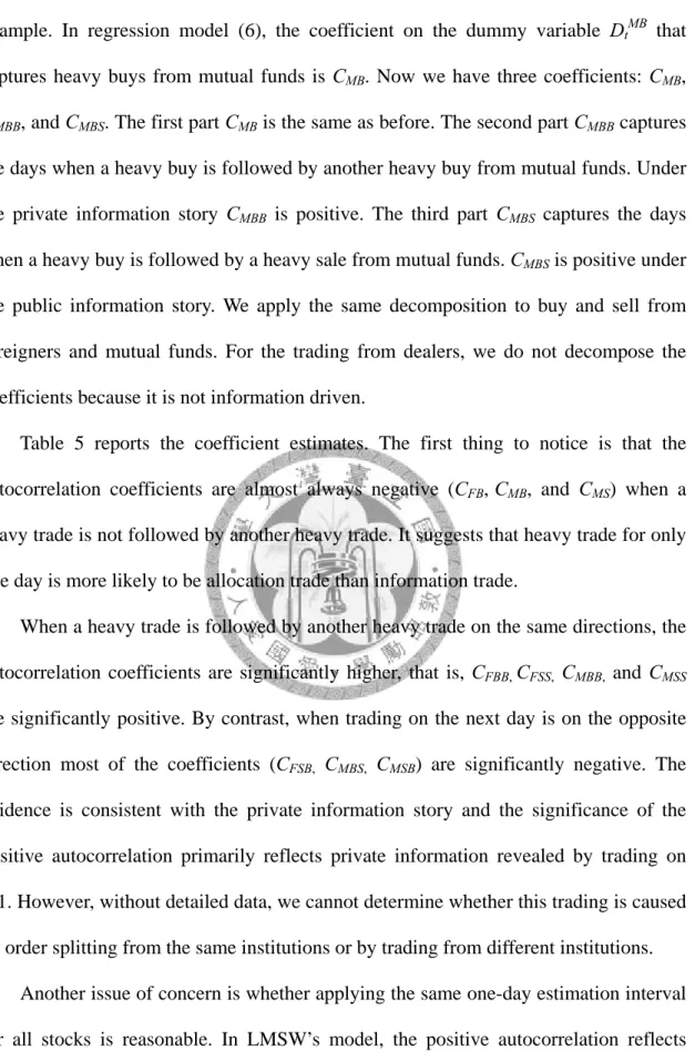
Rt+1 = C0 + C1Rt + C2VtRt + CFBDtFBDt[R>0]VtRt + CFSDtFSDt[R≦0]VtRt + CMBDtMBDt[R>0]VtRt+ CMSDtMSDt[R≦0]VtRt + CDBDtDBDt[R>0]VtRt+
CDSDtDSDt[R≦0]VtRt + εt+1, (6)
Rt+1 = C0 + C1Rt + C2VtORt + CFBQtFBDt[R>0]Rt + CFSQtFSDt[R≦0]Rt + CMBQtMBDt[R>0]Rt+ CMSQtMSDt[R≦0]Rt + CDBQtDBDt[R>0]Rt+ CDSQtDDt[R≦0]Rt + εt+1. (7)
We use a two step procedure to estimate coefficients in models (6) and (7). The first step is to run time-series regression for each stock to get the OLS estimate of coefficients. When any one group of institutional investors does not trade a given stock at all, its dummy variable is removed from the regression. We then estimate a cross-sectional average of the coefficients by running a robust regression that has only the intercept term. We use the STATA software rreg command to estimate the intercept.
A robust regression estimate is designed to deal with extreme observations with statistical validity. It is a form of weighted least-squares that first drops the most influential observations and then imposes smaller weights on observations with larger absolute residuals (Baker and Hall, 2004; Li, 1985). We have also estimated the mean with winsorizing or trimming at the 5th and 95th percentiles, the results are very similar.
3.2 Data
The availability of data on the trading volumes of institutional investors determines our sample period. The sample period begins on December 12, 2000, the day when local markets began to disclose the daily number of shares bought and sold by three groups of institutional investors – foreigners, mutual funds, and dealers. The sample period ends on March 30, 2007, and includes 1,558 trading days in total. To be included in the
sample, stocks are required a minimum number of 750 daily observations.5 The final sample includes 1,049 common stocks traded on the TSE or the over-the-counter market.
The data source is the Taiwan Economic Journal Database.
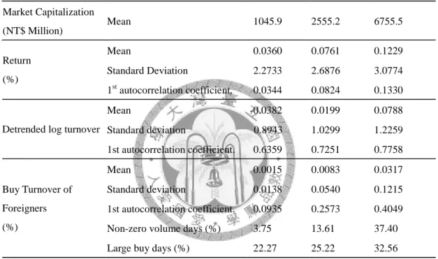
Table 1 reports the summary statistics for the variables used. We first calculate the time-series statistics of the variable of interest for each stock, and then report its 25th, 50th (median), and 75th percentiles across stocks. Because buy and sell from institutions have similar statistics, we choose to report the statistics for buy volume only.
Daily returns are positively autocorrelated. The first-order autocorrelations of daily returns are predominantly positive: the 25th percentile is 0.03 and the median is 0.08.
The positive autocorrelations suggest that the market takes time to reflect information.
Trading in Taiwan is strongly autocorrelated. Although not reported, the first-order autocorrelation of the daily turnover is high, with a 25th percentile of 0.64. The detrending procedure (deduct the 200-day moving average) does not reduce the autocorrelation. Table 1 reports that the 25th percentile of the first-order autocorrelation of the detrended log turnover is still 0.64.
Trading from institutional investors is less autocorrelated than other investors. The medians of autocorrelation coefficients from the three groups of institutional investors range from 0.24 to 0.36. Part of the positive autocorrelation of institutional trading is caused by order splitting (Lee, Liu, Roll, and Subrahmany, 2004).
Institutions do not trade very often. The median of the percentage of non-zero days is only 6% for mutual funds. It means that, for more than half of the sample stocks, mutual funds do not make any purchases on 94% of the trading days. Compared with other institutions, dealers trade more frequently. But even dealers do not make any
5 There are 185 stocks which are deleted due to this requirement. We have also tried to require a minimum number of 450 daily observations and obtained similar results.
Table 1: Summary Statistics
For each stock, we estimate statistics using its time-series data. Then we compute the quartiles of these statistics across stocks. Turnover is the number of total shares traded divided by the number of shares outstanding, and buy turnover is the shares bought divided by the number of shares
outstanding. The sample includes 1,049 stocks for which there are at least 750 daily observations and that were listed on the Taiwan Stock Exchange and the Gre Tai Securities Market. The sample period is from 2000/12/12 to 2007/3/30.
Variable Statistics Quartile1 Median Quartile3
Market Capitalization (NT$ Million)
Mean 1045.9 2555.2 6755.5
Mean 0.0360 0.0761 0.1229
Standard Deviation 2.2733 2.6876 3.0774 Return
(%)
1st autocorrelation coefficient. 0.0344 0.0824 0.1330
Mean -0.0382 0.0199 0.0788
Standard deviation 0.8943 1.0299 1.2259 Detrended log turnover
1st autocorrelation coefficient. 0.6359 0.7251 0.7758
Mean 0.0015 0.0083 0.0317
Standard deviation 0.0138 0.0540 0.1215 1st autocorrelation coefficient. 0.0935 0.2573 0.4049 Non-zero volume days (%) 3.75 13.61 37.40 Buy Turnover of
Foreigners (%)
Large buy days (%) 22.27 25.22 32.56
Mean 0.0007 0.0077 0.0297
Standard deviation 0.0109 0.0520 0.1231 1st autocorrelation coefficient. 0.2411 0.3630 0.4519 Non-zero volume days (%) 0.66 6.21 22.27 Buy Turnover of
Mutual Funds (%)
Large buy days (%) 18.71 22.63 28.73
Mean 0.0009 0.0050 0.0164
Standard deviation 0.0097 0.0308 0.0639 1st autocorrelation coefficient. 0.1486 0.2797 0.3911 Non-zero volume days (%) 3.45 18.79 37.74 Buy Turnover of
Domestic Dealers (%)
Large buy days (%) 22.43 25.86 31.56
purchase on 81% of the trading days for more than half of the sample stocks.
Institutional trades are concentrated on the days they trade. Take the buy turnover of mutual funds as an example; its standard deviation is 0.052%, which is more than six times larger than the mean (0.0077%) and suggests the existence of large trades. Given that heavy trades are unusual, these trades have the potential to move the price as the LSMW model suggests. To identify heavy trades from mutual funds, we use its 200-day moving average as the benchmark. On average, 22.6% of trading days are identified as heavy buy from mutual funds. Similarly, 25.2% and 25.9% of trading days are identified as heavy buys from foreigners and dealers.
4. Empirical Results
We begin by presenting empirical results for two basic regression models. Then we examine whether the autocorrelation reflects market information, industry information, or idiosyncratic information. We also examine whether the autocorrelation reflects public or private information.
4.1 Basic Results
To test the time-series implications of the LMSW model, we first estimate regression model (6). In model (6), the autocorrelation on days of heavy institutional buy or sell is estimated separately using dummy variables. Table 2 reports the estimation results. Panel A lists the average over all firms.
The 1st column of Panel A reports the average estimated from a robust regression.
We first look at the coefficient C2, which is the marginal autocorrelation coefficient on the days when the trading of institutional investors is low. The coefficient estimate is 0.003 and is not significantly different from zero. By contrast, on the days when
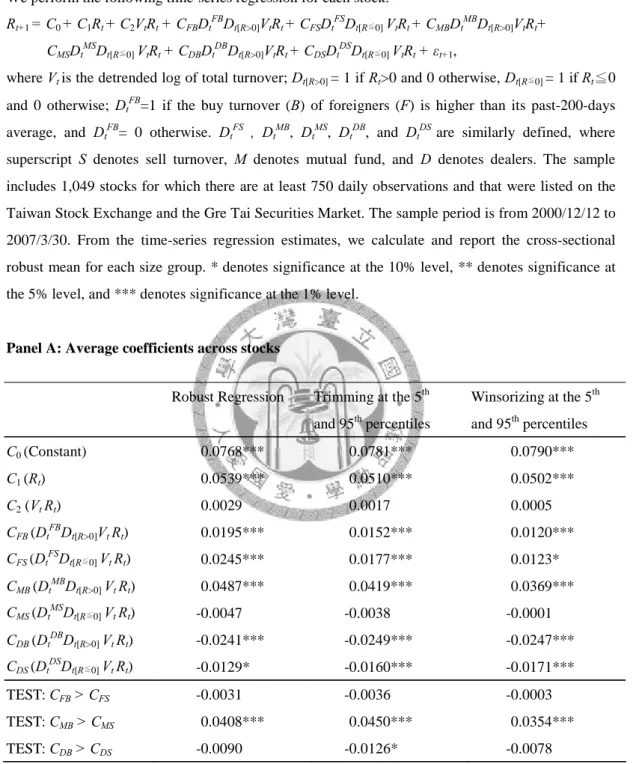
Table 2: Autocorrelation as a Function of Dummy Variables Constructed from Buy and Sell Volume from Institutional Investors
We perform the following time-series regression for each stock.
Rt+1 = C0 + C1Rt + C2VtRt + CFBDtFBDt[R>0]VtRt + CFSDtFSDt[R≦0] VtRt + CMBDtMBDt[R>0]VtRt+ CMSDtMSDt[R≦0] VtRt + CDBDtDBDt[R>0]VtRt+ CDSDtDSDt[R≦0] VtRt + εt+1,
where Vt is the detrended log of total turnover; Dt[R>0] = 1 if Rt>0 and 0 otherwise, Dt[R≦0] = 1 if Rt≦0 and 0 otherwise; DtFB=1 if the buy turnover (B) of foreigners (F) is higher than its past-200-days average, and DtFB= 0 otherwise. DtFS , DtMB, DtMS, DtDB, and DtDS are similarly defined, where superscript S denotes sell turnover, M denotes mutual fund, and D denotes dealers. The sample includes 1,049 stocks for which there are at least 750 daily observations and that were listed on the Taiwan Stock Exchange and the Gre Tai Securities Market. The sample period is from 2000/12/12 to 2007/3/30. From the time-series regression estimates, we calculate and report the cross-sectional robust mean for each size group. * denotes significance at the 10% level, ** denotes significance at the 5% level, and *** denotes significance at the 1% level.
Panel A: Average coefficients across stocks
Robust Regression Trimming at the 5th and 95th percentiles
Winsorizing at the 5th and 95th percentiles
C0 (Constant) 0.0768*** 0.0781*** 0.0790***
C1 (Rt) 0.0539*** 0.0510*** 0.0502***
C2 (Vt Rt) 0.0029 0.0017 0.0005
CFB(DtFBDt[R>0]Vt Rt) 0.0195*** 0.0152*** 0.0120***
CFS(DtFSDt[R≦0] Vt Rt) 0.0245*** 0.0177*** 0.0123*
CMB(DtMBDt[R>0] Vt Rt) 0.0487*** 0.0419*** 0.0369***
CMS(DtMSDt[R≦0] Vt Rt) -0.0047 -0.0038 -0.0001
CDB(DtDBDt[R>0] Vt Rt) -0.0241*** -0.0249*** -0.0247***
CDS(DtDSDt[R≦0] Vt Rt) -0.0129* -0.0160*** -0.0171***
TEST: CFB > CFS -0.0031 -0.0036 -0.0003
TEST: CMB > CMS 0.0408*** 0.0450*** 0.0354***
TEST: CDB > CDS -0.0090 -0.0126* -0.0078
foreigners or mutual funds trade heavily, the average marginal autocorrelation coefficients are significantly higher. For example, the average marginal autocorrelation coefficient on days with a heavy buy from mutual funds is C2+CMB, where CMB is 0.049 and is significantly positive. This is consistent with the LMSW prediction that
Table 2: (continued)
Panel B: Average coefficients across stocks within each size quartile
1st Quartile The Smallest
2nd Quartile 3rd Quartile 4th Quartile The Largest C0 (Constant) 0.0456*** 0.0774*** 0.0868*** 0.0923***
C1 (Rt) 0.0340*** 0.0607*** 0.0652*** 0.0444***
C2 (Vt Rt) 0.0513*** 0.0172*** -0.0164*** -0.0493***
CFB(DtFBDt[R>0]Vt Rt) -0.0323** -0.0068 0.0236*** 0.0608***
CFS(DtFSDt[R≦0] Vt Rt) 0.0084 0.0020 0.0345*** 0.0396***
CMB(DtMBDt[R>0] Vt Rt) 0.0163 0.0420*** 0.0542*** 0.0488***
CMS(DtMSDt[R≦0] Vt Rt) -0.0381 0.0093 0.0121 -0.0217*
CDB(DtDBDt[R>0] Vt Rt) -0.0443*** -0.0349** -0.0129* -0.0201***
CDS(DtDSDt[R≦0] Vt Rt) -0.0476** -0.0009 -0.0258** 0.0037 TEST: CFB > CFS -0.0364 -0.0097 -0.0043 0.0202*
TEST: CMB > CMS 0.0306 0.0170 0.0445*** 0.0673***
TEST: CDB > CDS -0.0123 -0.0237 0.0156 -0.0229*
information trading will generate positive autocorrelations.
The next question is whether buy volume has a different autocorrelation pattern from sell volume. The test results are reported in the last three rows of Panel A. For foreigners, the coefficient on days with heavy sell (CFS estimate is 0.025) is no different from the days with heavy buy (CFB estimate is 0.020). On the other hand, the coefficient on days with heavy sell from mutual fund (CMS) is -0.005. It is significantly smaller than the coefficient on days with heavy buy (CMB estimate is 0.049). The evidence on mutual funds supports our hypothesis that, due to short-sale constraints, sell volume contains less information than buy volume.
Dealers behave very differently from foreigners and mutual funds. The average autocorrelation coefficients on days with heavy trades from dealers are significantly negative. This evidence is consistent with our ex-ante identification that trading from dealers is less information driven than from foreigners and mutual funds.
In addition to estimating the average using a robust regression, we have also tried other methods to reduce the influence of extreme observations. The 2nd column of Panel A of Table 2 reports the average estimates after trimming the sample at the 5th and 95th percentiles; column 3 gives the average estimated by winsorizing at the same percentiles.
The estimates from three methods are very similar. Therefore, in the following we will only report the average estimated from robust regressions.
Panel B of Table 2 reports the average coefficients of four size quartiles. The average coefficients on Vt*Rt are negative for large firms and positive for small firms.
This cross-sectional pattern is similar to LMSW’s findings and consistent with their hypothesis that trading is more information driven for small firms, which have more information asymmetry.
The cross-sectional pattern of autocorrelation coefficients on days with heavy institutional trading is very different. When foreigners or mutual funds trade heavily, the average coefficients for large firms are significantly positive, but the coefficients for small firms are not. Therefore, institutions trade on information of large firms, not small firms. This evidence is consistent with the argument that the incentive to gather private information is stronger for large firms because institutional investors can trade large positions to make a profit. This is also consistent with findings in the literature that foreigners and mutual funds prefer to invest in large firms (Falkenstein, 1996; Kang and Stulz, 1997).
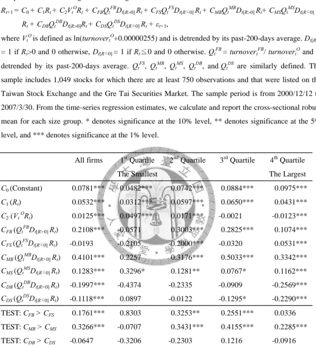
We also test the LMSW model using the regression model (7) which directly employs institutional volume in the regression rather than dummy variables. Table 3 reports the estimation results. Qualitatively, the results are very similar to Table 2 except that the difference between buy and sell volume is stronger in Table 3. For foreigners, high sell volume does not come with a higher average autocorrelation coefficient for the
Table 3: Autocorrelation as a Function of Buy and Sell Volume from Institutional Investors
We perform the following time-series regression for each stock.
Rt+1 = C0 + C1Rt + C2VtORt + CFBQtFBDt[R>0] Rt + CFSQtFSDt[R≦0] Rt + CMBQtMBDt[R>0] Rt+ CMSQtMSDt[R≦0]
Rt + CDBQtDBDt[R>0]Rt+ CDSQtDSDt[R≦0] Rt + εt+1,
where VtOis defined as ln(turnovertO+0.00000255) and is detrended by its past-200-days average. Dt[R>0
= 1 if Rt>0 and 0 otherwise, Dt[R≦0] = 1 if Rt≦0 and 0 otherwise. QtFB= turnovertFB/ turnovertO and is detrended by its past-200-days average. QtFS, QtMB, QtMS, QtDB, andQtDS are similarly defined. The sample includes 1,049 stocks for which there are at least 750 observations and that were listed on the Taiwan Stock Exchange and the Gre Tai Securities Market. The sample period is from 2000/12/12 to 2007/3/30. From the time-series regression estimates, we calculate and report the cross-sectional robust mean for each size group. * denotes significance at the 10% level, ** denotes significance at the 5%
level, and *** denotes significance at the 1% level.
All firms 1st Quartile The Smallest
2nd Quartile 3rd Quartile 4th Quartile The Largest C0 (Constant) 0.0781*** 0.0482*** 0.0742*** 0.0884*** 0.0975***
C1 (Rt) 0.0532*** 0.0312*** 0.0597*** 0.0650*** 0.0431***
C2 (Vt ORt) 0.0125*** 0.0497*** 0.0171*** -0.0021 -0.0123***
CFB(QtFBDt[R>0] Rt) 0.2108*** -0.0571 0.3003*** 0.2825*** 0.1074***
CFS(QtFSDt[R≦0] Rt) -0.0193 -0.2105 -0.2000*** -0.0320 0.0531***
CMB(QtMBDt[R>0] Rt) 0.4101*** 0.2257 0.3176*** 0.5033*** 0.3342***
CMS(QtMSDt[R≦0] Rt) 0.1283*** 0.3296* 0.1281** 0.0767* 0.1162***
CDB(QtDBDt[R>0] Rt) -0.1997*** -0.4374 -0.2335 -0.0909 -0.2569***
CDS(QtDSDt[R≦0] Rt) -0.1118*** 0.0897 -0.0122 -0.1295* -0.2290***
TEST: CFB > CFS 0.1761*** 0.8303 0.3253** 0.2551*** 0.0336 TEST: CMB > CMS 0.3266*** -0.0707 0.3431*** 0.4155*** 0.2285***
TEST: CDB > CDS -0.0647 -0.3206 -0.2303 0.1216 -0.0916
whole sample. Rather, it comes with a significantly lower average autocorrelation coefficient for one of the small firm quartiles. For both foreigners and mutual funds, there is strong evidence that buy volume contains more information than sell volume.
By contrast, there is no significant difference between buy and sell from dealers, who do not face the short-sale constraint. Hence, our evidence supports the hypothesis that the short-sale constraint will reduce the information content of sell volume.
4.2 Robustness Checks
When we test the significance of the average coefficient in Tables 2 and 3, we assume zero correlations between coefficients. This assumption is not correct if the error terms from the 1st step time-series regressions are correlated across stocks. To reduce the cross-sectional correlation between error terms, we follow Jorion (1990) to add the market return (MR) and the industry return (IR) to the time-series regressions as follows:
Rt+1 = C0 + C1Rt + C2VtRt + CFBDtFBDt[R>0]VtRt + CFSDtFSDt[R≦0] VtRt +
CMBDtMBDt[R>0]VtRt + CMSDtMSDt[R≦0] VtRt + CDBDtDBDt[R>0]VtRt+ CDSDtDSDt[R≦0] VtRt + C3 MRt+1 +C4 IRt+1+ εt+1.. (8)
Column (1) of Table 4 reports the coefficient estimates of model (8). The coefficients on market return and industry return are both significantly positive, but their significance does not change the significance of institutional trading. Results in Table 4 are very similar to Table 2. Therefore, our inferences are not driven by the cross-sectional correlation.
Results in Table 4 also suggest that trading by foreigners and mutual funds are based on firm-specific information rather than market or industry wide information.
Including the market and industry returns in the regression scarcely changes the coefficients on institutional trading. For example, the coefficient on foreigner (mutual fund) buying is 0.0195 (0.0487) in Table 2, and 0.0136 (0.0406) when market and industry returns are included with regressions in Table 4.
Including the market and industry returns in the regression does not guarantee the