邊界標記在註解系統之應用

(1)

國立臺灣大學電機資訊學院電機電信電子產業研發碩士專班碩士論文

邊界標記在註解系統之應用

吳湘筠

指導教授：顏嗣鈞教授

中華民國

國立臺灣大學電機電信電子產業研發碩士專班

Industrial Technology R&D Master Program in Electrical, Communication and Electronics Engineering

College of Electrical Engineering and Computer Science

National Taiwan University Master Thesis

碩士論文邊界標記在註解系統之應用吳湘筠撰

Boundary Label Placement and Its Application to Text Annotation

Wu, Hsiang-Yun

Advisor: Yen Hsu-Chun, Professor

97 年 7 月

97

7

July, 2008

(2)

i

口試委員會審定書

(3)

ii

誌謝

當論文寫到這一頁時，表示一切已經進入尾聲。能完成這篇論文，雖然幾經波折，但終於也看見了盡頭。我要特別感謝我的指導教授顏嗣鈞老師給予的指導與支持，以及口試委員雷欽隆老師、郭斯彥老師、黃秋煌老師、莊仁輝老師的批評與指教，也要感謝實驗室的每一位成員對我的支持與鼓勵，謝謝大家。

感謝實驗室的學長學弟們，在我如同熱鍋上的螞蟻時，適時給我鼓勵與安慰，

特別感謝春成學長在緊急時刻對我不離不棄，感謝學長紹祁、建良、克仁、成典、

柏源、紀憲、健生的鼓勵與支持，同學佑叡、亭遠、積瑞、昱鈞的照顧與幫助，

以及學弟秉賢、奕廷的拔刀相助，讓我終於順利地完成這篇論文。感謝我的家人在我情緒不穩定的時期，沒有給予我莫大的壓力，反而是默默地守護者我，感謝大學同學穎雯、嘉翎、若蘭的打氣，還有高中麻吉小光婷、趙孝的鼓勵，雖然每個人都有不同的阻礙與困難，但是卻願意陪我聊聊排解煩悶，真的很讓人感動。

最後，要感謝的人實在太多，如有被遺忘的朋友在此亦一併感謝，感謝大家於這兩年來對我的照顧，畢業雖不是人生的終點，卻是個完美的中場落幕。僅此論文獻給你們，願與大家一同分享這份喜悅。

謹誌於國立台灣大學電機工程研究所中華民國九十七年六月

(4)

iii

中文摘要

在資訊視覺化的研究領域，邊界標記被應用在許多不同的地方。一種常見的邊界標記形式包含一個定點及其對應的一個標籤，且這個標籤被放置在整個地圖的外圍上。在某些邊界標記應用領域，被標示的定點可能會分成多個群組連接到一個標籤或者一個定點連接至多個標籤亦或者多對多的情況，在這裏我們討論的

是一對一的情況。這篇論文裡，我們討論如何使用邊界標記法來改進

的註解系統。我們提供一個多項式時間的演算法來解決單一邊界的註解系統，此時可以藉由連結線段的彎曲來做視覺上的改進。我們也討論如何在雙邊標記上，平均最小化標籤的高度以及最小化連結線段的長度，也就是說，這個問題的目的是為了找出一個好的標籤排列方法，使得標籤高度最小，而連結線段的長度也最短。我們採用的連結線段的方式是垂直-平行-垂直(由零條或兩條垂直

線段跟一條水平線段所組成)連結邊界的方式，而這個問題具有的複

雜度。因此，我們採用了在計算數學中用於解決最優化的搜索演算法遺傳演算法來解決這個問題。在這篇論文裡的所提及的問題，我們假設連結線段是連接在標籤的正中間，換句話說，也就是擁有固定的連接點。這個雙邊界標記的問題是標籤配置和圖形繪製的綜合體，是個有趣且值得探討的問題。

在 Microsoft

Office Word

NP-complete

(5)

iv

ABSTRACT

Boundary labeling which can be found in many applications is an important field of information visualization. A conventional boundary labeling scheme connects one site to a unique label placed on the boundary of the drawing. In certain applications of boundary labeling, however, sites may be grouped or separated into more than one group and connect to an identical label on a picture or in an article with abundant numbers of sites and labels. We consider a special formula which includes one site and one identical label here.

In this thesis, we try to improve the annotation system of Microsoft Office Word by using boundary labeling solving methods. We provide a polynomial time solution to solve one-side annotation while the leader can be wound, and rerouted to improve the visualization. We also consider the label height minimization problem and leader length

minimization for two-side boundary labeling of the annotation system, i.e. the problem of finding a good leader and label placement, such that the number of total label height and total leader length is minimized. We proved that the two-side labeling problem for

type-opo leaders (rectilinear lines with either zero or orthogonal segment and one parallel segment) is NP-complete. Then, we give a heuristic genetic algorithm and

(6)

v

analyze its properties for the problems. For all the problems in this thesis, we assume that the connecting label ports are fixed ports, i.e. the point where each leader is connected to the label is fixed.

These problems are interesting in that it is a mixture of a label-placement and a graph-drawing problem.

(7)

vi

口試委員會審定書誌謝

中文摘要

LIST OF FIGURES

Figure 1-1: A sample article of Microsoft Office Word. ... 4

Figure 2-1: Type-s leader. ... 12

Figure 2-2: Types of leaders. ... 13

Figure 2-3: Types of many-side labeling. ... 14

Figure 2-4: Type-opo leader on two-side labeling. ... 16

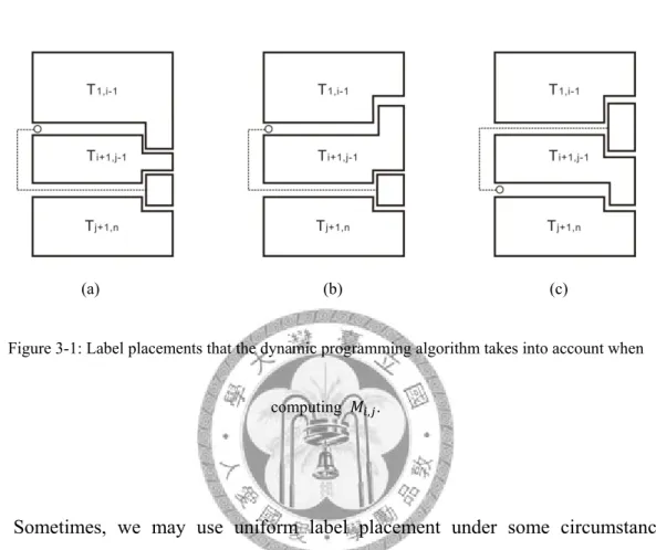
Figure 3-1: Label placements that the dynamic programming algorithm takes into account when computing , . ... 21

Figure 3-2: Transformation to two-side labeling on a line. ... 26

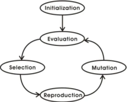
Figure 4-1: The basic loop of a genetic algorithm. ... 30

Figure 4-2: Four chromosomes represented as a 20-bits vector. ... 38

Figure 4-3: Four chromosomes represented as a 20-bits vector in iteration (i). ... 39

Figure 4-4: Type-opo leader of GA solution on two-side labeling. ... 40

Figure 4-5: Type-opo leader of optimal solution on two-side labeling. ... 40

Figure 5-1: Easy sample result of non-uniform rectangular label placement. ... 43

Figure 5-3: Type-opo leader of optimal s l ti n on two-side labeo u o ling. ... 45

Figure 5-4: The GA convergence with λ1 1.0 and λ2 0.0^U ... 46

Figure 5-6: Type-opo leader of optimal s l ti n on two-side labeo u o ling. ... 48

Figure 5-7: The GA convergence with λ1 0.0 and λ2 1.0^U ... 49

Figure 5-9: Type-opo leader of optimal so u io on two- ide abel t n s l ling. ... 51

Figure 5-10: The GA convergence with λ1 0.5 and λ2 0.5.^U ... 53

Figure 5-11: Sample result while the number of labels is small. ... 55

Figure 5-12: Sample result while the number of labels is large. ... 56

(10)

ix

Figure 5-13: Applicable sample result of our GA algorithm. ... 58 Figure 5-14: Sample result from Figure 5-13 ... 59

(11)

x

LIST OF TABLES

Table 1: Running time for related algorithms in big-O-notation. ... 8 Table 2: Details of our GA algorithm and optimal solution with λ =1.0 and λ =0.0. .. 44 1 2 Table 3: Details of our GA algorithm and optimal solution with λ =0.0 and λ2=1.0. .. 47 1 Table 4: Details of our GA algorithm and optimal solution with λ1 = λ2 = .5. ... 50 0 Table 5: Average experiment results of minimum leader length with various λ

combinations running 1000 times. ... 53 Table 6: Details of our GA algorithm and optimal solution on Word... 57 Table 7: Average results of our GA algorithm and comparison with optimal solution while

running 1000 times. ... 58

(12)

1

Chapter 1 Introduction

Label placement is one of important fields of information visualization. The majority of map labeling algorithms are also easily applicable for graph labeling. So, in diagrams, maps, technical or graph drawings, features like points, lines, and polygons must be labeled to convey information. The interest in algorithms that automate this task has increased with the advance in type-setting technology and the amount of information to be visualized. Due to the computational complexity of the label-placement problem, which is NP-hard in general [4], cartographers, graph drawers, and computational geometers have suggested numerous approaches, such as expert systems [15], zero-one integer programming [4], approximation algorithms [8],

(13)

2

simulated annealing [16] and force-driven algorithms [10] to name only a few.

At the beginning, we should distinguish between three kinds of graphical features according to their dimension.

(a) Point Features: Like cities, summits, area features on small scale maps, and vertices of graphs or diagrams.

(b) Line Features: Like rivers, boarders, streets, straight edges, polygonal lines, and edges or arcs of graphs or diagrams.

(c) Area Features: Like mountains, islands, and lakes.

Point and line feature labels are arranged next to the object and area feature labels usually placed within the boundary of the feature to be labeled.

Some rules are devised to measure the semantic clarity of a labeling assignment.

We state three concepts that are widely accepted as the basic rules for accurate map labeling.

Readability: The labels are of legible size.

Un-ambiguity: Each graphical feature of the map can be identified with the

corresponding label.

Avoidance of Overlaps: Labels should not overlap with other labels or other graphical

feature of the layout (map).

We denote the possible label positions of a feature as its label candidates.

(14)

3

Sometimes, a cost is assigned to an individual label candidate that reflects the quality of this label in terms of un-ambiguity, overlap with graphical features, and preferences between the label candidates.

Research on map labeling has been primarily focused on labeling point features, where the basic requirement is that the labels should be pairwise disjoint. It is clear that this is not achievable in the case of large labels. Large labels are common in technical drawings or medical atlases where certain site-features are explained with blocks of text.

To address this problem, Bekos et al. defined boundary labeling [4] and investigated some criteria, like minimizing the total leader length, in boundary labeling [5][6]. In boundary labeling, labels are attached on the boundary of a rectangle R which encloses all sites [4]. In their research, the main task is to place the labels in distinct positions on the boundary of R so that they do not overlap and, to connect each site with its corresponding label by non-intersecting polygonal lines, so called leaders.

Most of the problems of boundary labeling are one feature point corresponds to one label. And the main criteria are to place the labels in distinct positions on the boundary of R so that they do not overlap, or minimizes total leader length, or minimizes number of bends. But often some map or drawing not only connects exact one feature point to exact one label, but also connects several feature points to exact one label. Like the religion distribution in each state of a country, the language distribution

(15)

of the world, or the association or organization composed of some countries in Europe of Asia. But, in this thesis, we deal with labeling dense point sets with large labels and only one point can be allowed connecting to one label. The idea of this problem comes from the annotation system of Microsoft Office Word (See Figure 1-1). In the annotation system of Microsoft Office Word, we can easily find out that the leader of every site is composed of two straight lines. One is underline, and other connects to the corresponding label, and they are both dotted lines.

Figure 1-1: A sample article of Microsoft Office Word.

4

(16)

5

In some situation, this annotation system is not always good visually. Especially, when the number of sites grows larger; the number of labels also grows larger; one column is not enough for all of them. According to Figure 1-1, Microsoft Office Word puts all labels in one page, and it only supports 36 labels. When we want to place more than 36 labels, they will vanish on the page. Also, when there are lots of labels, labels with large index number will be far away from where corresponding sites are. If this happened, the dotted lines will be too close to recognize them. It is not a proper placement for the annotation system.

Our problem can be modeled as follows: we assume that we are given a set P = {p1,

p2,…, pn} of points and an axis-parallel rectangle R that contains P. Each point, or site,

pi is associated with an axis-parallel rectangular label and we only allow one point connecting to one label. The labels have to be placed and connected to their corresponding sites by polygonal lines, so-called leaders, such that no two labels intersect and the labels lie outside R. We investigate various constraints concerning the location of the labels and the type of leaders. More specifically we either allow attaching labels to one, and two sides of R, and we either compare straight line or rectilinear leaders. Our goal is placing labels such that crossings are not allowed. First, we will introduce an algorithm that could minimize all the distances between a site and its corresponding label for the annotation system. Then, we expand the problem to

(17)

6

two-side labeling problems while sites numbers are large. We show some problems in our model are NP-complete, and propose heuristic genetic algorithm to solve them.

In this thesis, we deal with labeling dense point sets with comparatively large labels. In the first half parts of this thesis, we try to normalize all the label size and fit them only on one side, and in the last half parts of this thesis, we separate labels into two groups. The same problem occurs when several locations on a map are to be labeled with large labels that must not occlude the map. The labels have to be placed and connected to their corresponding sites by polygonal lines, so-called leaders, such that (a) no two labels intersect, (b) no two leaders intersect, and (c) the labels lie outside R (boundary of the map) but touch R. We investigate some constraints concerning the location of the labels and the type of leaders. We consider two ways for visualization.

By using rectilinear leaders, namely type-opo leader that consists of two orthogonal and one axis-parallel segments. We show the complexity of this problem in Chapter 3. For details refer to Chapter 4, we model two-side boundary labeling problem on the famous heuristic algorithm “Genetic algorithm”. First, find some non-intersecting (i.e. feasible) leader-label placement, and we also consider two natural objectives: minimize the total length of the leaders [5][6] and minimize the total height of the labels that are too hard to solve at the same time.

This thesis is structured as follows. In chapter 2, we introduce some preliminary

(18)

7

knowledge associating our problems, including defining and modeling general boundary labeling problems. In chapter 3, we provide a new method by changing the order of labels to solve one-side annotation system. We also study the problem of minimizing total label height and total leader length when type-opo leaders are used and the labels are placed on left and right side of R. We proved these two problems are NP-complete. In chapter 4, we model the two-side labeling problem of minimizing total label height and total leader length with type-opo leaders on famous genetic algorithm.

Because the number of labels on left side and right side are not fixed, the problem is hard. We show this problem can be run on genetic algorithm under some constraints.

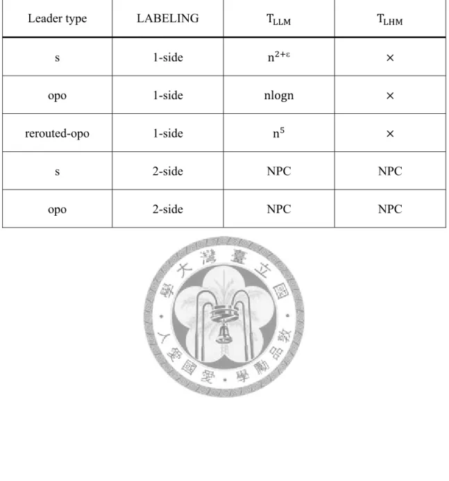
We show this heuristic algorithm is reasonable and suitable. In chapter 5, we simulate the problem with different parameters which may affect the result easily. Then, we analyze why they are accessible and compare the answer with optimal results of minimizing total label height and leader length at the same time. In chapter 5, we also show how these boundary labeling problems applied on Microsoft Office Word properly. At the end of this thesis; in chapter 6; we provide conclusions and introduce future work. All our surveys and works can be sum up in Table 1:

(19)

8

Table 1: Running time for related algorithms in big-O-notation.

Leader type LABELING T_LLM T_LHM

s 1-side n ^ε

opo 1-side nlogn

rerouted-opo 1-side n

s 2-side NPC NPC

opo 2-side NPC NPC

(20)

9

Chapter 2 Preliminaries

In boundary map labeling, the labels are placed in the boundary of the map that encloses all sites. To describe our problem in the thesis, we define the model of boundary labeling. We can choose what sides that the labels are placed to. The size of labels could be uniform or non-uniform. Boundary labeling is a kind of label placement that is usually used in cartography. However, we can also find out that it can also be used on article annotation as described before. Boundary labeling can be defined briefly as follow: A rectilinear map R with a lot of sites which are needed to be labeled.

(21)

10

2.1 Boundary Labeling Model

There are several variants in the boundary labeling model [4]. We try to introduce some below:

Side: Sides of the enclosing rectangle next to which we place labels. We can use any

sequence of N, E, W, and S (for North/East/West/South). In the cast of multiple stacks, we use NiEjWkSl when the labels are attached to the North, East, West, and South side of R and use i, j, k, l number of stacks, respectively. If no labels are placed next to a side we omit the letter corresponding to that side, and if only one stack is used we omit index 1.

LabelSize: UnifSize (all labels have the same size), MaxSize (all labels are Uniform of

MaxSize) or NonUnifSize (each label li is associated with a height hi and a width wi).

LabelPort: FixedPorts (points where a leader can touch a label are predefined) or

SlidPorts (points can slide along the label’s edge).

LabelPos: FixedPos (labels have either to be aligned with a predefined fixed set of

points on the boundary of the rectangle) or SlidePos (labels can slide along the rectangle’s sides)

Leader: Type of the leader (opo, po, or o). We’ll introduce it in next section.

Site: Type of the sites. Each site is a 1-point, line, rectangle, a polygon etc. In this thesis

(22)

11

we study that each site is a 1-point.

Objective: LEGAL (just find a legal label placement), TLLM (find a legal label

placement, such that the total leader length is minimum), TLHM (find a legal label placement, such that the total label height is minimum), TBM (find a legal label placement, such that the total number of bends is minimum or, equivalently, the number of type-o leaders is maximum), LSM (find the maximum label size for which a legal label placement is possible).

2.2 Types of Leaders

2.2.1 Straight-Line Leaders

Each leader is drawn as a straight line segment (see Figure 2-1). According to the

previous classification scheme, we refer to straight leaders as type-s leaders.

(23)

Figure 2-1: Type-s leader.

2.2.2 Rectilinear Leaders

A rectilinear leader consists of a sequence of axis-parallel segments that connects a site with its label. Each leader consists of a sequence of axis-parallel segments, which are either parallel (p) or orthogonal (o) to the side of R to which the associated label is

attached. This suggests that a leader c of type c1c2 . . . ck, where ci ∈ {o, p} consists of

an x- and y-monotone connected sequence (s1, s2, . . . , sk) of segments from the site to

the label, where segment si is parallel to the side containing the label if ci = p; otherwise

it is orthogonal to that side. Our primary focus has been on opo and po leaders

(see Figure 2-2 ), respectively.

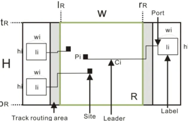
In this thesis we focus on leaders of the type opo (see Figure 2-2 (a)). For each type-opo leader we further insist that the central p-segment is immediately outside the

12

(24)

bounding rectangle R and is routed in a so-called track-routing area (see Figure 2-2 (b)).

We assume that the width of the track-routing area is fixed and large enough to accommodate all leaders with a sufficient distance. Due to this assumption the total length of the o-segments of all leaders is identical in all label-leader placements. Thus we are left with optimizing the length of the p-segments. Minimizing the width of the track-routing area for a given minimum leader distance is an interesting problem in itself, which is not the topic of this work.

(a) Type-po leader. (b) Type-opo leader.

Figure 2-2: Types of leaders.

2.3 Two-Side Labeling and Four-Side Labeling

Without losing generality, it is reasonable that we should not only put labels on one

13

(25)

side boundary of R. We should also think about other ways of putting them around R.

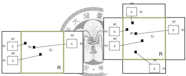
For examples, two-side labeling (see Figure 2-3 (a)), four-side labeling (see Figure 2-3 (b)), and circular labeling problems are also famous problem required to be studied. In this thesis, we studied more about two-side labeling problem which can be commonly used on the article annotation system, subway line labeling problem [9], and other applications.

(a) Type-s leader on two-side labeling. (b) Type-s leader on four-side labeling.

Figure 2-3: Types of many-side labeling.

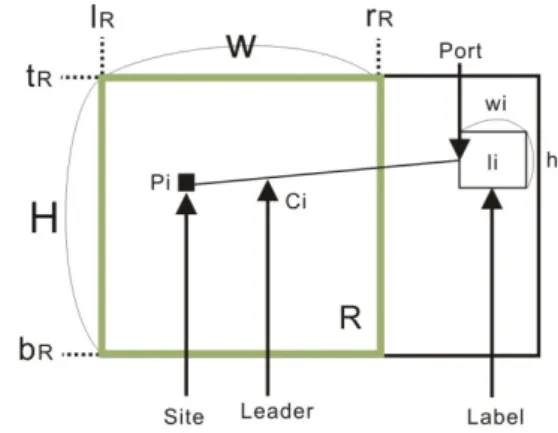
2.4 Modeling Two-Side Boundary Labeling

We consider the following problem. Given an axis-parallel rectangle R = [lR,

rR]×[bR, tR] of width W = rR –lR and height H = tR − bR, and a set P R of n sites pi

14

(26)

15

= (xi, yi ), each associated with an axis-parallel rectangular open label li of width wi and height hi , our task is to find a legal or an optimal leader-label placement. Our criteria for a legal leader-label placement are the following:

1. Labels have to be disjoint.

2. Labels have to lie outside R, close to the boundary of R.

3. Leader ci connects site pi with label li for 1 i n.

4. Intersections of leaders with other leaders, sites or labels are not allowed.

5. The ports where leaders touch labels may be fixed (the center of a label edge).

In this thesis we present a polynomial time algorithm to solve one-side rerouted leader problem and a genetic algorithm that computes legal leader-label placements (for brevity, simply referred to as labelings) for two-side labeling shown below (see Figure 2-4), but we also compare optimal placements of two-side label placement according to the following two objective functions:

z Balance label height (minimum total label length of two side) and z Short leader length (minimum leader length).

(27)

Figure 2-4: Type-opo leader on two-side labeling.

16

(28)

17

Chapter 3 One-Side Rerouted Leader and Two-Side Label Placement

We consider the problem about how to improve the annotation system of Microsoft Office Word. The criterion; total leader length; plays an important role in this problem, because we would like to place the label as near as its corresponding site. The criterion makes senses and it is practicable. In this chapter we focus on computing label placements of minimum total leader length and minimum total label height. We present an algorithm that attaches labels to one side (right) with rerouted leaders that change the order of labels. This is a new idea different from the original label placement. In two opposite sides (left and right), we prove that they are both NP-Complete problem for

(29)

18

satisfying either two objects described before. We also examine uniform and non-uniform labels, and fixed or sliding ports.

3.1

One-Side Rerouted-Leader Label Placement

In this section, we focus on computing label placement with rerouted leader and place all labels on one side (right side). The main point of our dynamic algorithm is how to compare total leader length of all label permutation efficiently. When there is a rerouted leader happened, we can find that the rerouted leader separates labels into three groups (see Figure 3-1 (a)). We have to calculate the sum of leader length of these three groups separately and compare with the length value while connecting to all labels through the right boundary, i.e. if rerouted leaders happened, the total leader length should be improved.

We employ a table S of size n n to maintain leader length minimization. We use table S to save all the possible placement of the first rerouted leader. Since the location of each label is fixed, the length of the leader to the ith label of s is determined. In the case of fixed port we define Right(p,i) to be the distance from site p to the port of the ith label of s . While in the case of sliding ports Right(p,i) is defined as the distance from site p to the closest point of the ith label of s . On the other hand,

(30)

19

Left(p,i) is defined similarly. In the case of fixed port we define Left(p,i) to be the distance from site p with rerouted leader to the port of the ith label of s . While in the case of sliding ports Left(p,i) is defined as the distance from site p to the closest point of the ith label of s with rerouted leader. We obtain the following results.

Theorem 1: Given a rectangle R of sufficient size, one sides r of R, a set P R of n

sites in general position and a non-uniform rectangular label for each site, there is an

O( )-time algorithm that attaches the labels to r and connects the site with

non-intersecting type-opo leaders or rerouted type-opo leaders to the corresponding

leaders using fixed or sliding ports such that the total number of leader length is

minimized.

Proof: Without the loss of generality, assume that s is the right side and s is the left side of rectangle R. We also assume that the sum of the label heights is at most the height of constant number N (in the annotation system, we may assume N as the height of a paper sheet) and that the sites are sorted according to increasing y-coordinate.

Recall that by p x , y we denoted the ith site, by h we denote the height of the

ith label, 1 i n, and by b_R and t_R we denote the y-coordinate of the bottom right and top right corner of R, respectively. Also, we denote _, as the length of

(31)

20

leader segment of kth leader in x-coordinate (orthogonal) direction and _, (parallel) as in y-coordinate direction. _, is defined as all possible combination of the first rerouted leader, i.e. we have to decide the most outside rerouted leader first, or we cannot implement our algorithm because of unstable label positions. For example, _, means that we choose site 8 and reroute its leader for the purpose of placing its label into the position 3. _, satisfies the following recurrence relation for 0 , . We can get , in polynomial time when we have already decided where label placed.

, _, _, , _, _, _, ,

In this algorithm, when we know how rerouted leader placed, we can separate labels into three groups (see Figure 3-1). The algorithm satisfies optimal substructure property which can be proved by contradiction. We assume that _, is minimum in our

solution. If there exist another _, _, _, , is

smaller than ∑ _, _, , we will choose _, as minimum solution. This contradicts to our assumption. Also, the algorithm satisfies overlapping sub-problem property (see Figure 3-1 (b) (c)). When we place the label of ith site to jth position or when we place the label of jth site to ith position, we will count the same sub-problem of _, and _, . The worse case of this algorithm happens when the leader always

(32)

reroutes to the most outside of the sub problem. So, the complexity is ∑

.

(a) (b) (c)

Figure 3-1: Label placements that the dynamic programming algorithm takes into account when

computing , .

Sometimes, we may use uniform label placement under some circumstances.

However, this problem is easier than previous one. We don’t need to add more information about label sizes and where labels placed in this situation.

Theorem 2: Given a rectangle R of sufficient size, one sides r of R, a set P R of

n sites in general position and a uniform rectangular label for each site, there is an

O( )-time algorithm that attaches the labels to r and connects the site with

non-intersecting type-opo leaders or rerouted type-opo leaders to the corresponding

21

(33)

22

leaders using fixed or sliding ports such that the total number of leader length is

minimized.

We can prove this theorem by adding more information of labels from Theorem 1.

The way of calculating , is easier. The displacement of labels is constant when reroute happens (see Figure 3-1). We can save tiny time from previous one while sites are little.

3.2 Label -Height Minimization on Two-Side Labeling

Without losing generality, when we try to improve the annotation system, we would like to separate labels into two groups averagely. Which means it’s better to separate labels into two groups, and these two groups have the same label height. In this two-side map boundary labeling problem, we are given a map G = (S, L), S is a set of sites, L is a set of corresponding labels, and a positive integer M= Total label height , a finite set H which represents all the label height in L, and a target t. As usual, we define the problem as a language Two-Side Labeling: {<H,M,t>: there exists subsets H^′ H such that min ∑ _H′h M t }

(34)

23

Instance: A map G = (S, L), S is a set of sites, L is a set of corresponding labels, and a positive integer M = Total label height , a finite set H which represents all the label height in L, and a target t.

Question: Does there exist a subset of L that total height of labels is the nearest height vale to M?

Theorem 3: Minimizing label height of Two-Side map boundary labeling with opo-leader is NP-complete.

Proof: To show that two-side labeling is in NP, for an instance <H,M,t> of the problem, we let the subset H^′ be the certificate. Checking whether ∑ _H′h M t can be accomplished by a verification algorithm in polynomial time. To show the NP-hardness of this problem, we will reduce it from the subset sum problem. We will show that SUBSET-SUM p TWO-SIDE BOUNDARY LABELING problem. When t=0, this problem is equal to subset sum problem absolutely. We have to whether there exists a subset H^′ H such that ∑ _H′h M. While t=1,2,…,n, we also have to check whether there exist a H^′ H satisfies ∑ _H′h M t. This is also another subset problem. If we want to solve this problem, we have to solve subset sum problem many time until we find the minimum t. On the other hand, if we can solve this problem,

(35)

24

we can find out a corresponding subset sum problem. To sum up, TWO-SIDE BOUNDARY LABELING is NP-hard and TWO-SIDE BOUNDARY LABELING is in NP. TWO-SIDE BOUNDARY LABELING is a NP-Complete problem.

3.3 Leader-length Minimization on Two-Side Labeling

Leader-length minimization of two-side labeling is another criterion of our solution.

Without losing generality, when we try to improve the annotation system, we would like to place labels as near its’ site as possible. Which means it’s better to minimize leader length to fit the object.

Instance: Given k , and a set S of n sites on many horizontal lines of set L. Each site has rectangular label with dimension w h . And a set R={r the shortest length from site s to the right boundary}

Question: If there exist any legal opo-labeling with labels on left side and right side of a boundary R, such that the total leader length is at most M?

Theorem 4: Minimizing total leader length of Two-Side map boundary labeling with opo-leader is NP-complete.

(36)

25

Prof: In order to prove the problem belongs to NP-complete problem. We need to guess a position of the labels on the boundary of L and also check (i) the label do not overlap each other. (ii) all the leaders do not intersect with each other. (iii) the sum of leader length is no more than M. We can reduce the problem of determining a legal solution of partition model.

Given positive integers p , p , … , p , is there a subset I of J={1,2,…,2m}such that I contains exactly one of {2i-1,2i} for i=1,2,…,m, and ∑ _Ia ∑ _J/Ia? We will reduce an instance P of partition problem to an instance(S,L) of this problem such that P can be partitioned if and only if there is a two-side boundary labeling of S with corresponding labels to L. This problem can be reduced as a problem that there are many sites on one vertical line, and we want to put all the labels on right side or left side.

If there are more than one sites on the horizontal line, we can assume that they are different sites and very close on the target vertical line (see Figure 3-2). At the same time, every site is lying on the central of the line where it is placed.

(37)

26

Figure 3-2: Transformation to two-side labeling on a line.

We can easily prove this problem by reducing partition problem to it. Giving an integer set A={a , a , … , a } which represents the length of p-segment of every pairs of sites and labels. Also because all the sites have the same distance to the boundary, we can get another integer set B; while b B, and let

b a length of L width of track routing area

Then, we can easily apply this problem to partition which is well-known as a NP-complete problem. Whereas, and if we can find an answer of two-side boundary labeling problem, we can also get the answer of corresponding partition problem. So, minimizing total leader length of Two-Side map boundary labeling with opo-leader is NP-complete.

Because both label height minimization and leader length minimization are NP-Complete problem. And when we try to solve one of both problems, we will not

(38)

27

also get the optimal solution of the other. If we want to solve both of the problems at the same time, it will be harder than solving one problem. So, we try to use genetic algorithm to solve two problems at the same time and runs quickly.

(39)

28

Chapter 4 Genetic Algorithm on Two-Side Labeling

Genetic algorithms are stochastic global search methods that have proved to be successful for many kinds of optimization problems. Genetic algorithms are categorized as global search heuristics. These algorithms work with a population of candidate solutions and try to optimize the answer by using three basic principles, including selection, crossover (also called recombination), and mutation. The initial population should be chosen randomly. Then, during subsequent generation, new candidate solutions are produced by selecting two individuals, with higher probability of selection for better individuals. And then, we have to recombine parts of these individual to form one or two offspring, and mutate (change slightly) the resulting offspring. At last, the

(40)

29

new descendent is inserted back to the population and worst individual is deleted.

Genetic algorithm can be shown as follow:

Pseudo-code algorithm

1. Choose initial population

2. Evaluate the fitness of each individual in the population 3. Repeat

(a) Select best-ranking individuals to reproduce

(b) Breed new generation through crossover and mutation (genetic operations) and give birth to offspring

(c) Evaluate the individual of the offspring

(d) Replace worst ranked part of population with offspring 4. Until termination

The basic loop is depicted in (see Figure 4-1). The implement of all steps will be discussed in more detail in Chapter 4.

(41)

Figure 4-1: The basic loop of a genetic algorithm.

4.1 Genetic Algorithm Modeling

Genetic algorithms are implemented as a computer simulation in which a population of abstract representations (called chromosomes or the genotype or the genome) of candidate solutions (called individuals, creatures, or phenotypes) to an optimization problem evolves toward better solutions. Traditionally, solutions are represented in binary as strings of 0s and 1s, but other encodings are also possible. The evolution usually starts from a population of randomly generated individuals and happens in generations. In each generation, the fitness of every individual in the population is evaluated, multiple individuals are stochastically selected from the current population (based on their fitness), and modified (recombined and possibly randomly mutated) to form a new population. The new population is then used in the next iteration of the algorithm. Commonly, the algorithm terminates when either a maximum number

30

(42)

31

of generations has been produced, or a satisfactory fitness level has been reached for the population. If the algorithm has terminated due to a maximum number of generations, a satisfactory solution may or may not have been reached.

Genetic algorithms find application in bioinformatics, phylogenetics, computer science, engineering, economics, chemistry, manufacturing, mathematics, physics and other fields.

A typical genetic algorithm requires two things to be defined:

1. a genetic representation of the solution domain, 2. a fitness function to evaluate the solution domain.

A standard representation of the solution is as an array of bits. Arrays of other types and structures can be used in essentially the same way. The main property that makes these genetic representations convenient is that their parts are easily aligned due to their fixed size, which facilitates simple crossover operation. Variable length representations may also be used, but crossover implementation is more complex in this case. Tree-like representations are explored in Genetic programming and graph-form representations are explored in Evolutionary programming.

The fitness function is defined over the genetic representation and measures the

quality of the represented solution. The fitness function is always problem dependent.

For instance, in the knapsack problem we want to maximize the total value of objects

(43)

32

that we can put in a knapsack of some fixed capacity. A representation of a solution might be an array of bits, where each bit represents a different object, and the value of the bit (0 or 1) represents whether or not the object is in the knapsack. Not every such representation is valid, as the size of objects may exceed the capacity of the knapsack.

The fitness of the solution is the sum of values of all objects in the knapsack if the representation is valid or 0 otherwise. In some problems, it is hard or even impossible to define the fitness expression; in these cases, interactive genetic algorithms are used.

Once we have the genetic representation and the fitness function defined, GA proceeds to initialize a population of solutions randomly, and then improve it through repetitive application of mutation, crossover, inversion, and selection operators.

4.1.1 Individual

The individual represent a candidate solution. In this problem, it represents a legal label placement without crossing. The individuals are stored as real-valued vector. We let the element “0” of the vector representing connecting to left side boundary. On the other side, the element “1” means putting label to the right side boundary. Although it is conceivable that different genetic representations influence the optimization behavior significantly, we choose this representation instinctively. Because we only need two

(44)

33

types of groups to represent connecting to the left side or connecting to the right side, it is obviously that binary integer representation is just what we need.

4.1.2 Initialization

At the beginning of the genetic algorithm, the individuals in the population have to be initialized. Initially many individual solutions are randomly generated to form an initial population. The population size depends on the nature of the problem, but typically contains several hundreds or thousands of possible solutions. Traditionally, the population is generated randomly, covering the entire range of possible solutions (the

search space). Occasionally, the solutions may be "seeded" in areas where optimal solutions are likely to be found. In our case, this is done randomly. We generate a label placement with restricted given area (including rectangle R, track routing area, and space for labels) and let bad offspring eliminated by selection.

4.1.3 Evaluation

The choice of the evaluation function plays a crucial role in the design of a genetic algorithm. There is a big advantage of using evaluation in genetic algorithm. One can

(45)

34

measure desired criteria on the resulting placement and weight these criteria to suit personal preferences. Because genetic algorithm is always using in multi-purpose problem, we can then analyze how important these criteria are.

Among the criteria we test are

• All the leaders do not cross to each other.

• All the labels do not overlap to each other.

• Total labels should be placed balanced on left side and right side.

• The longer label height on left side and right side is minimum height.

• Total leader length is a minimum length of all combination.

The result presents in Chapter 5 show some cases of legal placement.

4.1.4 Selection

Selection is important to genetic algorithm, since only selection drives the search towards more promising regions of the search space. In our implementation, we select individuals for reproduction (i.e. parents) according to the common linear ranking selection scheme, i.e. individuals are selected according to their rank, with better individuals receiving a higher chance of being selected. So that, the selective pressure of actual fitness values, which may be important, since it is not known beforehand in

(46)

35

which range of fitness values the optimal solution is located. The algorithm is of the steady state type, i.e. the offspring is introduced into the population, and at least fit individual is deleted. This way, the best solution so far is never lost. Also, in our problem, when crossing happened, the individual should not be counted in the population.

We define fitness function as follow:

f λ ∑ c

n |t_R b_R| |r_R l_R| ε λ |R L |

R L

R Label height of the right side.

Label height of the left side.

: L :

ε: Track routing area width.

t : Top position of the boundary.

: Bottom position of the boundary.

R

b_R

r_R: Right position of the boundary.

l_R: Left position of the boundary.

In order to normalize the function, we divide these parameters to their intuitive maximum value. Thus without generality, λ and λ can be chosen between 0 and 1, and satisfy λ λ 1.

4.1.5 Recombination

(47)

36

In order to get better result, we combine two good parents into a new offspring which may be brown better or not. The purpose of the crossover operator is to recombining sub-placements of different individuals to produce an offspring. Since, we expect that good parts of a placement are connected, we perform crossover by choosing randomly a connected parts of the placement of two parents and swap the sub-placement.

However, unfortunately, there is a problem with this operator using this method. A combination of two good parents may yield a poor offspring. This poor offspring will be deleted during the natural selection process.

4.1.6 Mutation

Mutation is a crucial step of genetic algorithm. While using recombination, we can only find new combination of individuals that are already at present. We may lose some information forever while it is not in the population. Another method called mutation can introduce new material into the population, i.e. the slight changing of individuals. It is necessary and reasonable to get new materials to increase the probability of getting better answers. In out implementation, mutation is done by randomly changing binary vector with a given small probability. We try to change one leader from the right side to

(48)

37

left side (or from the left side to the right side). This way, we will have a probability to get a better individual through the present individual and the result is different from the recombination (or crossover) process.

4.2 An Example of GA on Two-Side Labeling

Now, we give a simple example how we implement genetic algorithm on two-side labeling. At the beginning, we give a fixed rectangle R which is 400 by 300 units as the target map and also give a fixed width for the track routing area that is assumed enough for all the leaders’ placement. Initially, we generate the number of sites, the height of labels randomly. Also, we can get some parameters (including R width, track routing area width and total label height) for the fitness function shown below:

f λ ∑ c

n |t_R b_R| |r_R l_R| ε λ |R L |

R L

After that, for the fitness function, we only need to calculate the length of leader of any possible placement generated from the algorithm and the combination of labels. We give 4 chromosomes represented as a 20-bits vector as an example (see Figure 4.2-1).

Letting the element “0” of the vector represents connecting to left side boundary. On the

(49)

other side, the element “1” of the vector represents connecting to right side boundary.

(see Figure 4.2-1)

38

chromosome [0]=10100110011101110101 fitness = 0.1946 chromosome [1]=01001101011111000011 fitness = 0.2077 chromosome [2]=11111011011111001110 fitness = 0.2359 chromosome [3]=10111010111001011011 fitness = 0.2335

Figure 4-2: Four chromosomes represented as a 20-bits vector.

In this genetic algorithm, we have to select smaller fitness number as better individuals, and this is different from original fitness definition. Then in iteration (i), we choose the smallest two individuals chromosome [0] and chromosome [1] and recombine them in order to get better offspring (see Figure 4.2-2). After recombination, we can find out that CrossOverChromosome [2] is better than its parents. In the program, choose a number of bits for swap process randomly. In this case, we choose first 4 bits of chromosome [0] and swap them to the first 4 bits of chromosome [1] and get chromosome [2] and chromosome [3]. As the result, one is better and the other is worse. It is obviously that the worse individuals will be eliminated by the natural selection in this iteration.

(50)

39

CrossOverChromosome [0] = 10100110011101110101 fitness = 0.1946 CrossOverChromosome [1] = 01001101011111000011 fitness = 0.2077 CrossOverChromosome [2] = 01000110011101110101 fitness = 0.1856 CrossOverChromosome [3] = 10101101011111000011 fitness = 0.2200

Figure 4-3: Four chromosomes represented as a 20-bits vector in iteration (i).

The iteration will stop when all the four individuals have the same chromosome. In this situation, we will ignore the possibility of mutation in the future because it is not worthy to wait for its happening. The mutation only occurs with a given small probability. In this algorithm we choose only a bit of vector and change it. Even this may not always useful in the algorithm, it helps when we need more different material in the population. The GA result and optimal result show below: (see Figure 4-4 and see Figure 4-5)

(51)

Figure 4-4: Type-opo leader of GA solution on two-side labeling.

Figure 4-5: Type-opo leader of optimal solution on two-side labeling.

40

(52)

41

Chapter 5 Simulation Results

For now, we test our algorithm on a number of example graphs with rerouted leader on one-side labeling and genetic algorithm on two-side labeling. As described above, there are some disadvantages of the annotation system of Microsoft Office Word.

While inputted label number is small, it is more general that users may want to enlarge label height to see more details in the labels. On the other hand, while inputted label number becomes larger, the system should not abandon labels easily. We provide the following method to prove the annotation system: (i) While inputting little labels, we enlarge label size to fit the height of paper sheet and apply the situation on rerouted leader labeling method. However; we can also use this method to prove the

(53)

42

visualization by combining dotted lines into one. We will show the detail in the following sections. (ii) While inputting many labels, we can also combine labels of sites on one line. (iii) While inputting many labels, in order to provide more space for labels, we try to reduce the space of text and provide one more column for labels in one page.

This way, we can apply the situation on two-side labeling problem. We separate them into three basic groups to see whether two objects: minimum label height and minimum leader length is important.

5.1 Rerouted Leaders on One-Side Labeling

Recall the details in chapter 3; we proved that the algorithm of rerouted leader label placement of one-side labeling is run in polynomial time O(n ). The total leader length of original placement is 1880 units and rerouted leader placement is 1120 units (see Figure 5-1). This one-side labeling problem with rerouted leaders makes the annotation system improvable. In next section, we will show how it looks when applying on Word.

(54)

(a) Original placement. (b) Rerouted leader placement.

Figure 5-1: Easy sample result of non-uniform rectangular label placement.

5.2 Genetic Algorithm on Two-Side Labeling

In this section, we slightly change λ and λ in order to get better visualization of two-side labeling problem. Besides, we also want to know how these parameters affect the final result.

5.2.1 Leader Length Minimization

In some situation, we may focus on object “leader length minimization”. We can slightly change λ and λ to fit our destination. So, we try typical formation to see how important they are under our constraints.

43

(55)

44

Table 2: Details of our GA algorithm and optimal solution with λ =1.0 and λ =0.0.

Total leader length Difference of label height

GA algorithm 5842 units 44 units

Optimal solution 4710 units 48 units

Here, the site number is 20, total leader length of Figure 5-5 is 5842 units and height difference of left labels and right labels is 44 units. Total leader length of Figure 5-6 is 4710 units and height difference of left labels and right labels is 48 units. In this case, we assume possible maximum leader length is 16020 units and total label height is 12080 units.

(56)

45

(57)

When these objectives are not both important, we may try to set with λ 1.0 and λ 0.0. This is reasonable for the normalization. We also show that the genetic algorithm works, because the average fitness converge to optimal fitness finally (see Figure 5-4). It converges quickly. Although in other cases, we may see some points which are not respected, it’s because the mutation process and we still can find out the tendency of convergence. Even though the leader length is smaller, it doesn’t look very good because the labels of two sides are not balanced as usual.

Figure 5-4: The GA convergence with λ 1.0 and λ 0.0

0 1 2 3 4 5 6 7 8 9 10

Best fitness 0.376 0.369 0.364 0.364 0.364 0.364 0.364 0.364 0.364 0.364 0.364 AVG fitness 0.411 0.385 0.373 0.367 0.364 0.364 0.364 0.364 0.364 0.364 0.364

0.34 0.35 0.36 0.37 0.38 0.39 0.4 0.41 0.42

GA convergence

46

(58)

47

5.2.2 Label Height Minimization

In some situation, we may focus on object “label height minimization”. We can slightly change λ and λ to fit our destination. So, we try typical formation to see how important they are under our constraints.

Table 3: Details of our GA algorithm and optimal solution with λ =0.0 and λ =1.0.

Here, the site number is 20, total leader length of Figure 5-5 is 6478 units and height difference of left labels and right labels is 28 units. Total leader length of Figure 5-6 is 6232 units and height difference of left labels and right labels is 0 units. In this case, we assume possible maximum leader length is 16020 units and total label height is 12080 units.

(59)

48

(60)

When these objectives are not both important, we may try to set with λ 0.0 and λ 1.0. This is reasonable for the normalization. We also show that the genetic algorithm works, because the average fitness converge to optimal fitness finally (see Figure 5-7). It converges quickly. Although in other cases, we may see some points which are not respected, it’s because the mutation process and we still can find out the tendency of convergence.

Figure 5-7: The GA convergence with λ 0.0 and λ 1.0

0 1 2 3 4 5 6 7 8 9 10

0 0.002 0.004 0.006 0.008 0.01 0.012 0.014 0.016

GA convergence

49

(61)

50

For the annotation system, we believe that two-side labeling can solve this problem.

If we use two-side labeling for the annotation system, we must reduce the number of words in one page, i.e. we need two column spaces for all the labels.

5.2.3 Leader Length and Label Height Minimization

In some situation, we may focus on both leader length and label height minimization. We can slightly change λ and λ to fit our destination. So, we try typical formation to see how they work under our assumption.

Table 4: Details of our GA algorithm and optimal solution with λ = λ = 0.5.

(62)

51

(63)

52

Here, the site number is 20, total leader length of Figure 5-8 is 6274 units and height difference of left labels and right labels is 28 units. Total leader length of Figure 5-9 is 4756 units and height difference of left labels and right labels is 8 units. In this

case, we assume possible maximum leader length is 16020 units and total label height is 12080 units.

When these objectives are both important, we may set λ and λ are 0.5 which is reasonable for the normalization. We also show that the genetic algorithm works, because the average fitness converge to optimal fitness finally (see Figure 5-10). It converges quickly. Although in other cases, we may see some points which are not respected, it’s because the mutation process and we still can find out the tendency of convergence. In this case, we can easily find out that these two objects are both important for beautiful placement.

(64)

Figure 5-10: The GA convergence with λ 0.5 and λ 0.5.

0 1 2 3 4 5 6 7 8 9 10

0.18 0.185 0.19 0.195 0.2 0.205 0.21 0.215 0.22 0.225

GA convergence

Table 5: Average experiment results of minimum leader length with various λ combinations running 1000 times.

λ λ , 1.0,0.0 0.9,0.1 0.8,0.2 0.7,0.3 0.6,0.4 0.5,0.5 0.4,0.6 0.3,0.7 0.2,0.8 0.1,0.9 0.0,0.1

L 5954.8 5780.6 6091.4 5756.6 5950.6 6036.0 5909.8 5961.2 5928.0 6134.4 6389.6

opt ⁴⁷¹⁰ ⁴⁷¹⁰ ⁴⁷¹⁰ ⁴⁷¹⁰ ⁴⁷¹⁰ ⁴⁷⁵⁶ ⁴⁷⁵⁶ ⁴⁷⁵⁶ ⁴⁷⁵⁶ ⁴⁷⁵⁶ ⁶²³²

% 0.2642 0.2273 0.2932 0.2222 0.2633 0.2691 0.2425 0.2534 0.2464 0.2898 0.0252

L ^69.0 ^80.0 ^65.2 ^77.6 ^72.0 ^78.0 ^58.4 ^73.2 ^20.2 ^27.2 ^24.6

opt ⁴⁸ ⁴⁸ ⁴⁸ ⁴⁸ ⁴⁸ ⁸ ⁸ ⁸ ⁸ ⁸ ⁰

% 0.4375 0.6666 0.3583 0.6166 0.5000 8.7500 6.3000 8.1500 1.5250 2.4000 #

Besides, we also try some other λ combinations (see Table 5). Because of different λ combinations, optimal solutions are also different. So, when we want to compare these data, we have to compare with their own optimal solutions. According

53

(65)

54

to Table 5, we can find out that there is a tendency that total leader length grows larger while focusing on label height balance, and vice versa. Even though the results of our algorithm depend on initial placement mostly, λ combinations still affect them. In fact, the best λ combination should be defined case by case, so we do not study them a lot.

5.3 Implementation on Word

In this section, we try to apply our abstract algorithm on real Office Word. Then, we will discuss the advantages and disadvantages of original word annotation system and our results.

5.3.1 Rerouted-Leaders on One-Side Labeling

We provide some sample results here. In order to improve this system, we tried many ways of using this annotation system. So, we encountered many difficulty of telling one leader from each other while there are too many labels on one page or when labels are far from their corresponding sites. For example (see Figure 5-11), there exists some big labels near the bottom of the boundary. This case makes labels above are placed higher than they expect. This placement is not easy to understand because

(66)

leaders are long and close to each other (see Figure 5-11 (a)). The main idea of our method is that we can rearrange the order of the labels (see Figure 5-11 (b)). We provided rerouted leaders and this method simplify the complexity of connecting pairs of sites and labels. The result showed follow looks quite good as we expected.

(a) Original label placement of MS Word. (b) Sample result of our algorithm.

Figure 5-11: Sample result while the number of labels is small.

Another situation is that users may need to annotate more than one word on one line (see Figure 5-12). This case is even worse on visualization than the case above. The placement is harder to understand because leaders are too close to each other (see Figure 5-12(a)). To simply the complexity, we combine labels on the same line together

55

(67)

(see Figure 5-12(b)), and only provide one leader to the combination labels. This way, we reduce the number of leaders and minimize total leader length which are both important for visualization. The result showed follow looks clear and more understandable.

(a) Original label placement of MS Word. (b) Sample result of our algorithm.

Figure 5-12: Sample result while the number of labels is large.

5.3.2 Genetic Algorithm on Two-Side Labeling

When site number grows larger, it will take too much time for searching optimal

56