行政院國家科學委員會專題研究計畫 成果報告
具不確定性之平面連桿機構瞬心位置解析解法之研究 研究成果報告(精簡版)
計 畫 類 別 : 個別型
計 畫 編 號 : NSC 97-2221-E-011-033-
執 行 期 間 : 97 年 08 月 01 日至 98 年 07 月 31 日 執 行 單 位 : 國立臺灣科技大學機械工程系
計 畫 主 持 人 : 王勵群
計畫參與人員: 碩士班研究生-兼任助理人員:蔣星苓 碩士班研究生-兼任助理人員:許智博 博士班研究生-兼任助理人員:龔哲民
處 理 方 式 : 本計畫可公開查詢
中 華 民 國 98 年 10 月 08 日
國科會研究計畫成果報告
計畫名稱: 具不確定性之平面連桿機構瞬心位置解析解法之研究 (I)
計畫編號: NSC 97-2221-E-011-033
計畫類別: 一般型研究計畫 (個別型)
主持人: 王勵群
執行單位:國立臺灣科技大學機械系
執行期間:2008/08/01 ~ 2009/07/31
An Analytical Method for Locating the Secondary Instant Centers of Indeterminate Planar Linkages (I)
Abstract
This report presents the first year’s results of the research project of developing a new analytical method for locating the secondary instant centers of indeterminate planar linkages. In this report, the secondary instant centers are first discriminated into three classes according to their level of geometric dependencies. The concepts of instant-center digraph, instant-center walk, and instant-center circuit are then introduced to establish the recursive relationships between the classified instant centers.
Keywords: instant center; indeterminate linkage; graph theory; analytical method
1. Introduction
The concept of instantaneous center of zero velocity (or instant center in short) is important for motion analysis of complex single degree-of-freedom (DOF) planar mechanisms, for the knowledge of which not only provides an easy and efficient way to obtain the instantaneous angular velocity ratio among the links, but also is useful for analyzing the mechanical advantage and configuration singularities of the mechanism [1]. It is well known that the location of instant centers of most of the single DOF planar linkages can be evaluated by using the Aronhold-Kennedy theorem.
However, for some of the linkages which consist of eight or more links, it is not sufficient based on the Aronhold-Kennedy theorem alone to locate all of their instant centers; such linkages are commonly known as the indeterminate linkages in the literature [2].
Several researchers have studied the kinematic characteristics of indeterminate linkages in the past and a number of different methods have been proposed for evaluating their instantaneous properties. Dijksman has presented a linkage reduction method through joint-joining operation to determine the instant centers and coordinated centers of curvature in network mechanisms, in which the double butterfly linkage is used as a demonstrative example [2, 3]. Foster and Pennock have developed a graphical method to find the secondary instant centers of the double butterfly linkage according to the unique direction of the velocity vector of special coupler points [4]. More recently, they have shown that a secondary instant center of a two DOF linkage must lie on a unique straight line and presented a new graphical technique to locate the secondary instant centers by converting single DOF indeterminate linkage into a two DOF one [5]. These methods, however, are based on the use of graphical techniques to replace the original linkage into a different kind of linkage, and hence may not be easily to be implemented on digital computers.
On the other hand, Gilmore and Cipra have developed an analytical method by using the vector loop closure equations and the idea of mechanism inversion to find the instant centers, centrodes, inflection circles, and centers of curvature of planar linkages [6]. Yan and Hsu have also utilized the velocity matrix to determine the location of unknown instant centers of complex mechanisms [7]. These methods do not rely on the Aronhold-Kennedy theorem and they are applicable to any planar mechanism including the indeterminate ones, but they require the evaluation of the derivatives of the vector loop closure equations of the mechanism to obtain the relative instant center of each pair of the movable links. Therefore it would be elaborate to use if the mechanism contains several coupled kinematic loops or only the locations of certain set of instant centers are required to be evaluated.
Based on the fact that the location of the instant centers of a single DOF planar linkage are independent of the selection of the input joint and its velocity; a new analytical method for locating the instant centers of indeterminate linkages which does not rely on any velocity information or graphical techniques is proposed in this research project. The proposed method consists of two parts and will be respectively developed in two years’time. In this first year’s report, the secondary instant centers of a given linkage are first classified into three classes according to the level of their geometric dependencies. Based on this classification and the use of the circle diagram, a directed graph, referred as the instant-center digraph, is introduced to discriminate the recursive relationships between the secondary instant centers. The breadth-first search algorithm is then applied to the graph for finding the occurrence sequences, referred as the instant-center walk, of these instant centers. In addition, a recursive formula for successively computing the coordinates of the instant centers in an instant-center walk is established.
2. Classification of the Secondary Instant Centers
As defined by Foster and Pennock [5], a primary instant center (PIC) of a linkage is referred to as the one which can be directly located by inspecting the kinematic structure of the linkage, such as those associated with permanent connections between the links. Those of which can not be directly located by inspection but should be deduced from the knowledge of other instant centers are referred to as the secondary instant center (SIC) of the linkage.
It is well known that a general method for locating the SICs of a given linkage is to use the circle diagram for book keeping and the Aronhold-Kennedy theorem to recursively evaluate these instant centers one by one by finding the intersection point of the two pole-lines (i.e. the straight line that constitutes the three instant centers of three links moving relative to one another) which both contains the instant center in question. However, for indeterminate linkages this method would be stalled at a point where no two related pole-lines can be found for an undetermined SIC and hence can not be carried out further. In order to discriminate this situation, in this paper, the SICs are further classified into three classes according to their level of dependencies.
To facilitate the follow up presentations, a PIC between links i and j is denoted as
J i,jand a SIC is denoted as Ii,j
. The first class of SIC of a given linkage is defined as
the ones that at least two independent pole-lines corresponding to them can be
obtained from the PICs of the linkage and, hence, their location is independent of
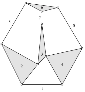
other SICs and can be readily evaluated. For example, the initial state of the circle
diagram of the single flier eight-bar linkage shown in Figure 1 is given in Figure 2,
from which it can be observed that the SICs I1,3
and I2,4
are of this class.
The second class of SIC is defined as the ones which only one of the corresponding pole-lines can be obtained from the PICs, such as I
2,6
of the single flier eight-bar linkage, since only one pole-line (i.e. the one connecting J2,5
and J5,6
)corresponding to it can be ascertained from Figure 2. Finally, the SICs of which none of the corresponding pole-lines can be determined from the PICs are defined as the third class. It can be observed from Figure 2 that only one among all of the SICs of the single flier eight-bar linkage is of this class and which is I
1,6
.It should be noted that, for single DOF planar mechanisms, once the positions of the first class SICs have been located based on the given configuration of the linkage and the PICs, they can then be treated as the PICs, and, consequently, the state of some of the second and/or the third class SICs can be upgraded to that of the first class and be evaluated accordingly. This process can be carried out repeatedly until either the position of all of the SICs have been evaluated, or none of the state of the reminding second and third class SICs can be upgraded. The later case would indicate that the given linkage is an indeterminate one.
3. Instant-Center Digraph and Instant-Center Walks
In order to further discriminate the dependencies between the undetermined second and third class SICs of indeterminate linkages, instant-center digraph and the concept of instant-center walk are introduced in this section.
An instant-center digraph is a directed graph in which the vertices are designated to the undetermined SICs and are denoted by using the same notation as the SIC. Any two vertices in the graph having a common subscript, such as I
i,j
and Ij,k
, may be connected by an edge, provided that they are not both of the third class SIC and that the instant center between links j and k is a PIC (i.e. Jj,k
). The direction of the edge is determined according to the following rules:1. If both of the two vertices are of the second class, then the edge is bidirectional and is represented by a two-way arrow. This is because, according to the
Aronhold-Kennedy theorem, these two SICs must lie on a pole-line defined by them together with J
j,k
, and this pole-line must be different from the known one of each of them. Therefore, if the location of either one of the pair of SICs is given, then that of the other can be determined as the intersection point of this pole-line and the one that already known.2. If one of the two SICs is of the third class and the other is of the second class, then the edge can only be directed from the third class one to the second class one but not vice versa. Since even if the location of the second class one is given, there still missing one pole-line to locate the position of the third class SIC.
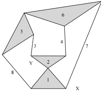
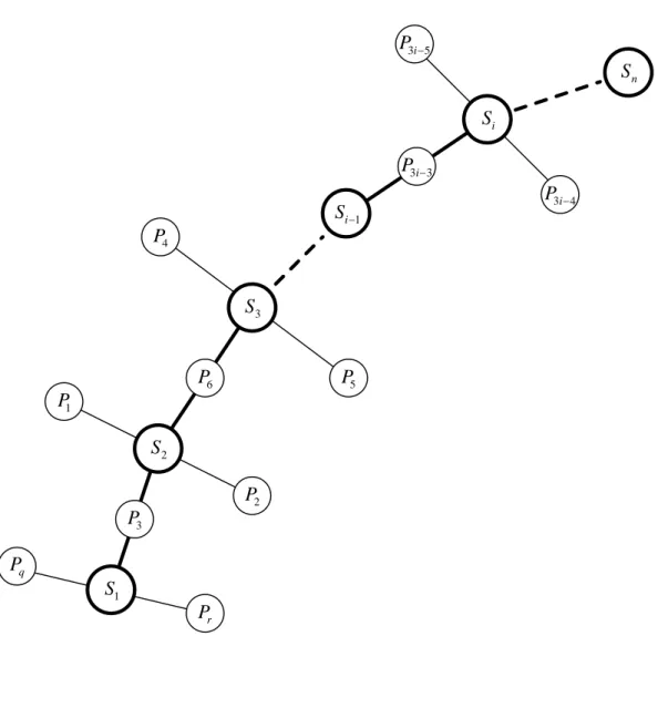
Based on the rules described above, the instant-center digraph of the double butterfly linkage shown in Figure 3 is constructed and illustrated in Figure 4 as an example. This linkage has a total of eighteen undetermined SICs, among them sixteen are of the second class and two are of the third class, as respectively enclosed in the graph by the symbols of ○ and △.
Once the instant-center digraph of an indeterminate linkage is constructed, the relationship between the undetermined SICs of it can be further established by instant-center walks. An instant-center walk is defined as a directed path from one SIC to another SIC in the instant-center digraph, such that each edge in the path is incident from the preceding vertex toward the following vertex, and no edge appears more than once. According to this definition and the rules for constructing the instant-center digraph, it can be concluded that, except the starting vertex, all of the SICs in an instant-center walk should be of the second class, for the edges incident with a third class SIC can only point outward from it. In addition, a closed instant-center walk in which the starting and the ending SIC are the same is referred to as an instant-center circuit, and it follows that it is not possible to form such circuit
for a third class SIC.
The instant-center walk gives a directed relationship between the two end vertices, and which, as will be shown in the next section, is useful for establishing a recursive computational scheme to evaluate the coordinates of the unknown instant centers. It should, however, be noted that the instant-center walk between two given vertices may not be uniquely defined. Nevertheless, in order to save computation time, it is desirable to find the walk which consists of the least amount of the intermediate vertices. This is known as the shortest path problem in the graph theory, which can be solved by several existing graph-theoretic algorithms. In this paper, the breadth-first search algorithm is employed to find the shortest instant-center walks [8].
4. Recursive Computational Scheme for Instant-Center Walk
Denoting the instant-center walk between two SICs, I
i,j
and Ik,l
, as { S1
, S2
, …, Si-1
,S i, Si+1
, …, Sn
}, where S1
= Ii,j
and Sn
= Ik,l
. Since S2
must be a second class SIC,
therefore one of its pole-line is known, and which can be written into the point-slope
form as
2, y 1 2, x 1
S = m S + c
, (1)where
, ,
, ,
1 y 2 y
1
1 x 2 x
p p
m p p
, (2)and
, , , ,
, ,
2 x 1 y 1 x 2 y
1
1 x 2 x
p p p p
c p p
. (3)In which (p
1,x
, p1,y
) and (p2,x
, p2,y
) are, respectively, the coordinates of the two PICs P1
and P
2
associated with the known pole-line of S2
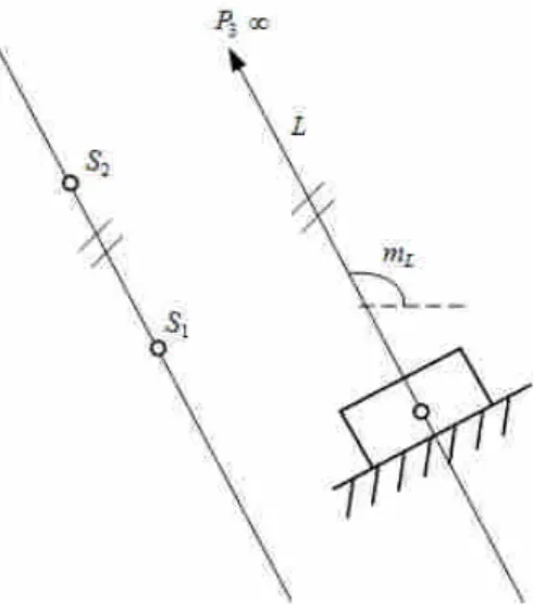
, as shown in Figure 5. In addition, according to the property of the instant-center walk, S2
must also lies on a pole-line defined by S1
and another PIC, P3
, as shown in the figure, which can also be written into the point-slope form as2, y 2 2, x 2
S = m S + c
, (4)where
1, 3,
2
1, 3,
y y
x x
S p
m S p
, (5)and
2 3, 1, 1, 3,
1, 3,
x y x y
x x
p S S p
c S p
. (6)In which (S
1,x
, S1,y
) denotes the coordinates of S1 . By simultaneously solving equations
(1) and (4), it follows that the coordinates of S2
can be written in terms of that of S1
as
2,2 1, 2,1 1, 2,0
2,
2,2 1, 2,1 1, 2,0
x y
x
x y
A S A S A
S B S B S B
(7)
2,2 1, 2,1 1, 2,0
2,
2,2 1, 2,1 1, 2,0
x y
y
x y
D S D S D
S B S B S B
. (8)
In which A
2,i
, B2,i
, and D2,i
, i = 0~2 are constant coefficients given by2,2
(2, x 1, y 1, x 2, y
)3, y
(1, x 2, x
)A =
p p
p p
p p
p
2,1 3, x
(1, x 2, x
)A = p p
p
2,0 3, x
(2, x 1, y 1, x 2, y
)A =
p
p p
p p
2,2
(1, y 2, y
)B =
p
p
2,1
(1, x 2, x
)B = p
p
2,0 3, x
(1, y 2, y
)3, y
(1, x 2, x
)B = p p
p
p p
p
2,2 3, y
(1, y 2, y
)D =
p p
p
2,1
(2, x 1, y 1, x 2, y
)3, x
(1, y 2, y
)D =
p p
p p
p p
p
2,0 3, y
(2, x 1, y 1, x 2, y
)D =
p
p p
p p
.It should be noted that equations (7) and (8) are derived based on the assumptions that both the slope of the pole line defined by P
1
and P2
and the locations of the PICs are finite. If p1,x
= p2,x
then the pole line would be perpendicular to the x axis of the reference frame and the slope m1
would become infinity. Nevertheless, in this case equation (1) can be replaced byx
x P
S 2 ,1
and which can be substituted into equation (4) to find the intersection point of the two lines. On the other hand, if P
3
is the instant center corresponding to a sliding pair as shown in Figure 6, then it would be located at infinity along the line L which is perpendicular to the sliding direction of the slider, and the pole-line defined by S1
, S2
, and P3
should be parallel to L. Therefore, by using the two-point form, equation (4) in this case can be modified toL x x
y
y m
S S
S
S
1 2
1
2
,where m
L
is the slope of line L. Again, ifm L then the equation above would be reduced to simply
x
x S
S 2 .1
It should also be pointed out that if the two pole-lines are coincided with each other, then equations (1) and (4) would become linear dependent and therefore no unique intersection point of the two lines can be determined. For example, the four PICs, J
12
, J23
, J34 , and J 14
of the four-bar linkage at the configuration illustrated in Figure 7 are lie on the same straight line, thus the SICs I13
and I24
can not be uniquely located without knowing the speed ratio of the input and the output link at the instance. Since this situation would only occur under certain singular configurations of the linkages having special link dimensions, and can only be handled by specifying additional velocity information of the linkage, therefore it is not dealt with in this paper and only the more general nonsingular cases are considered.By using the same procedure, the coordinates of the third SIC in the given walk,
S 3, can be written as functions of that of S2
as
3,2 2, 3,1 2, 3,0
3,
3,2 2, 3,1 2, 3,0
x y
x
x y
A S A S A
S B S B S B
(9)
3,2 2, 3,1 2, 3,0
3,
3,2 2, 3,1 2, 3,0
x y
y
x y
D S D S D
S B S B S B
, (10)
where
3,2
(5, x 4, y 4, x 5, y
)6, y
(4, x 5, x
)A =
p p
p p
p p
p
3,1 6, x
(4, x 5, x
)A = p p
p
3,0 6, x
(5, x 4, y 4, x 5, y
)A =
p
p p
p p
3,2
(4, y 5, y
)B =
p
p
2,1
(4, x 5, x
)B = p
p
2,0 6, x
(4, y 5, y
)6, y
(4, x 5, x
)B = p p
p
p p
p
3,2 6, y
(4, y 5, y
)D =
p p
p
3,1
(5, x 4, y 4, x 5, y
)6, x
(4, y 5, y
)D =
p p
p p
p p
p
3,0 6, y
(5, x 4, y 4, x 5, y
)D =
p
p p
p p
.In which (p
4,x
, p4,y
), (p5,x
, p5,y
), and (p6,x
, p6,y
) are the coordinates of the PICs P4
, P5
, and P6
corresponding to the known pole lines of S2
and S3
, as shown in Figure 5.Consequently, the functional relationship between the coordinates of two successive SICs, S
i
and Si-1
, i = 2 ~ n, in the given walk, can be written into the general form as,2 1, ,1 1, ,0
,
,2 1, ,1 1, ,0
i i x i i y i
i x
i i x i i y i
A S A S A
S B S B S B
(11)
,2 1, ,1 1, ,0
,
,2 1, ,1 1, ,0
i i x i i y i
i y
i i x i i y i
D S D S D
S B S B S B
, (12)
where
,2
(3 4, 3 5, 3 5, 3 4,
)3 3,
(3 5, 3 4,
)i i x i y i x i y i y i x i x
A =
p p p p p p p
p p p
,1 3 3,
(3 5, 3 4,
)i i x i x i x
A = p p p
,0 3 3,
(3 4, 3 5, 3 5, 3 4,
)i i x i x i y i x i y
A =
p p p p p
p p
,2
(3 5, 3 4,
)i i y i y
B =
p p
,1
(3 5, 3 4,
)i i x i x
B = p p
,0 3 3,
(3 5, 3 4,
)3 3,
(3 5, 3 4,
)i i x i y i y i y i x i x
B = p p p p p p
p p p
,2 3 3,
(3 5, 3 4,
)i i y i y i y
D =
p p p
,1
(3 4, 3 5, 3 5, 3 4,
)3 3,
(3 5, 3 4,
)i i x i y i x i y i x i y i y
D =
p p p p p p p
p p p
,0 3 3,
(3 4, 3 5, 3 5, 3 4,
)i i y i x i y i x i y
D =
p p p p p
p p
are constant coefficients in terms of the coordinates of the PICs P
3i-5
, P3i-4
, and P3i-3
shown in Figure 5.
Equations (11) and (12) give the basic recursive relationship between two successive SICs in a given instant-center walk, by recursively applying these equations from the first SIC to the i
th
SIC, the coordinates of any SIC in the walk can be expressed in terms of that of the first one as,2 1, ,1 1, ,0
,
,2 1, ,1 1, ,0
i x i y i
i x
i x i y i
U S U S U
S V S V S V
(13)
,2 1, ,1 1, ,0
,
,2 1, ,1 1, ,0
i x i y i
i y
i x i y i
W S W S W
S V S V S V
(14)
where
,2 ,2 1,2 ,1 1,2 ,0 1,2
i i i i i i i
U = A A A D A B
A B
,1 ,2 1,1 ,1 1,1 ,0 1,1
i i i i i i i
U = A A A D A B
A B
,0 ,2 1,0 ,1 1,0 ,0 1,0
i i i i i i i
U = A A A D A B
A B
,2 ,2 1,2 ,1 1,2 ,0 1,2
i i i i i i i
V = B A B D B B
B B
,1 ,2 1,1 ,1 1,1 ,0 1,1
i i i i i i i
V = B A B D B B
B B
,0 ,2 1,0 ,1 1,0 ,0 1,0
i i i i i i i
V = B A B D B B
B B
,2 ,2 1,2 ,1 1,2 ,0 1,2
i i i i i i i
W = D A D D D B
D B
,1 ,2 1,1 ,1 1,1 ,0 1,1
i i i i i i i
W = D A D D D B
D B
,0 ,2 1,0 ,1 1,0 ,0 1,0
i i i i i i i
W = D A D D D B .
D B .
In addition, if the first instant-center is a second class SIC, then as shown in Figure 5, it must lies on a known pole line defined by the two PICs, P
q
and Pr
, such thatS 1,y =m S 1,x +c,
(15) in which, ,
, ,
q y r y
q x r x
p p
m p p
,and
, , , ,
, ,
r x q y q x r y
q x r x
p p p p
c p p
.Consequently, by substituting equation (15) into (13) and (14) and rearranging terms, one obtains
,1 1, ,0
,
,1 1, ,0
i x i
i x
i x i
E S E
S G S G
(16)
and
, ,1 1, ,0
,1 , ,0
i x i
i y
i i x i
H S H
S G S G
, (17)
where
,1 ,2 ,1
i i i
E
U
U m
,0 ,1 ,0
i i i
E
U c U
,1 ,2 ,1
i i i
G
V V m
,0 ,1 ,0
i i i
G
V c V
,1 ,2 ,1
i i i
H
W
W m
,0 ,1 ,0
i i i
H
W c W
.Equations (16) and (17) are particularly useful for evaluating the locations of the SICs within an instant-center circuit, as will be shown in the next section.
5 Conclusions
A general analytical approach to locate the instant centers of indeterminate planar linkages has been developed. It is shown that the dependencies between the undetermined secondary instant centers of such linkages can be conveniently represented by a directed graph. Based on which the concepts of instant-center walk and instant-center circuit are introduced, and a recursive formula for computing the coordinates of the instant centers in an instant-center walk is established.
The proposed approach can be easily programmed on digital computers for automated analysis, and it can be systematically applied to all types of indeterminate linkages even when sliding pairs are presented. However, it should be noted that the presented method can only be applied to single DOF indeterminate linkages at nonsingular configurations. The possibilities of extending the method to handle singular configurations due to special link geometry and indeterminate linkages of multi DOF have not been investigated and are suggested as future research topics.
References
[1] A. G. Erdman, G. N. Sandor, and S. Kota, Mechanism Design Analysis and Synthesis, Volume 1, Fourth Edition, Prentice Hall, pp. 165-176
[2] E. A. Dijksman, Why Joint-Joining is Applied on Complex Linkages. Proceedings of the Second IFToMM International Symposium on Linkages and Computer Aided Design Methods 11(17) (1977) 185-212
[3] E. A. Dijksman, Geometric Determination of Coordinated Centers of Curvature in Network Mechanism through Linkage Reduction. Mechanism and Machine Theory 19(3) (1984) 289-295
[4] D. E. Foster, and G. R. Pennock, A Graphical Method to Find the Secondary Instantaneous Centers of Zero Velocity for the Double Butterfly Linkage. Journal of Mechanical Design 125 (2003) 268-274
[5] D. E. Foster, and G. R. Pennock, Graphical Methods to Locate the Secondary Instant Centers of Single-Degree-of-Freedom Indeterminate Linkages, Journal of Mechanical Design 127 (2005) 249-256
[6] B.J. Gillmore, and R. J. Cipra, An Analytical Method for Computing the Instant Centers, Centrodes, Inflection Circles, and Centers of Curvature of the Centrodes by Successively Grounding Each Link. Journal of Mechanisms, Transmissions, and Automation in Design 105 (1983) 407-414
[7] H-S. Yan, and M-H. Hsu, An Analytical Method for Locating Velocity Instantaneous Centers. Proceedings of the 22
nd
Biennial ASME Mechanisms Conference, Flexible Mechanism, Dynamics, and Analysis 47 (1992) 353-359 [8] Narsingh Deo, Graph Theory with Applications to Engineering and ComputerScience, Prentice Hall, 1974, pp. 268-327
Figure 1. Schematic Diagram of the Single Flier Eight-bar Linkage
Figure 2. Circle Diagram of the Single Flier Eight-bar Linkage
Figure 3. Schematic Diagram of the Double Butterfly Linkage
I
4,5I
2,7I
3,6I
2,5I
2,6I
1,6I
1,5I
3,8I
5,7I
6,8I
7,8I
3,7I
4,8I
3,4I
1,4I
4,7I
2,8I
1,3Figure 4. Instant-center Digraph of the Double Butterfly Linkage
S 1
P 1
P q
S 2
P 2
P 3
1
S i
S i
S n
3 i 3
P
P r
P 4
P 5
3 i 5
P
3 i 4
P
P 6
S 3
Figure 5. Recursive Relationship of the SICs in an Instant-center Walk
Figure 6. Parallel Pole-lines
Figure 7. Singular Configuration of a Four-bar Linkage