Motion Control Components’ Algorithms on a Chip for Driving Module

(1)

Motion Control Components’ Algorithms on a Chip for driving module

*Wen-yo Lee, Jhu-Syuan Guo Computer Information and Network Engineering

Lunghwa University of Science and Technology Taoyuan, Taiwan

*TristanWYLee@mail.lhu.edu.tw

Chi-Pin Chen

Intelligent Mechatronics Department/MSRL Industrial Technology Research Institute

Chutung, Hsinchu, Taiwan cpchen@itri.org.tw

Abstract—A motion control chip implementation method will be shown in this paper. The implementation is based on the Verilog HDL which is a popular tool for designing a special function FPGA, especially on the industrial field. There are several components needed in a control chip according to the motion control requirements. The major components are: encoder readers, PWM generators, subtracter/Adder, PID controller, as well as the communication ports. These algorithms have been developed on an FPGA, which is used to control an IR2100 based DC motor drive for a mobile robot. The IR2100 based drive is also been introduced for completing the article structure.

Finally, we will show you that the motion driving module is applied on a more than 50Kg mobile robot.

Keywords: FPGA, ; Controller Algoritm; Mobile robot;

I. INTRODUCTION

The motion controllers have been implemented for machine’s moving control for years [1-3]. A stand along machine system － a mobile robot, it requires a low cost constructing solution, high performance controller, and high reliability hardware. In general, a mobile robot consists of servo motors, stepping motors, sensors, controllers, and others.

The manufacturing cost will be the key issue of the competition on the market, so the best solution is to design these components of a mobile robot by the manufacturer. The basic components of a motion controller for a DC motor drive are encoder readers, PWM generators, subratcter, and an automatic control algorithm. For a stepping motor control, the pulse generator will be the major component. One can use the industrial made components for the study machines, but sometimes it is quite hard to fully implement your own ideas on your studies. Furthermore, the cost of the implementation will be rapidly increased by more and more special function requirements. Here the paper will show how to implement the motion controller components that can be referred to implement some studies, especially the automatic control algorithm. Some of the most important components of a motion controller are discussed in the following sections.

With powerful computing capability, a microcontroller is introduced to interpolate the motion control profile and generate the position pulses in motion control applications.

The acceleration and deceleration curve of a motion profile can be generated by computing the mathematic formula or by searching in a prepared lookup table. A non-DSP microcontroller with a 60M Hz clock, if it is taken to implement the software emulation for the floating point computation to calculate the interpolation of a motion profile, the maximum frequency of the output pulse will not exceed 100K Hz. That means the performance of the controller would be limited and may not handle a precision servo control.

On the other hand, if a microcontroller serves as a pulse generator for a stepping motor, it may not have extra capability to handle other process events of a system. A stand along pulse generator can be implemented by an FPGA (Field programmable gate array) [6-7]. Then, the microcontroller gives the commands: velocity, maximum acceleration, and total pulses, to the motion pulse generation chip; then the pulse generator generates the desired motion pulses in the type of T-type velocity profile for point-to-point motion control.

This paper is organized as follows. In section 2, the motion control components’ algorithms are discussed in detail.

In section 3, the simulation results are shown here. In section 4, the hands-on implementation and experiments are presented. Finally, the conclusions are briefly given in the final section.

II. THEMOTIONCONTROLCOMPONENTS’

ALGORITHMS

The motion control components can be fully implemented in an FPGA, since the high density gate count of the FPGA nowadays. The functions of the embedded controller on an FPGA can be separated into four blocks: the general purpose I/O, the communication ports, the motion controller, and the command parser.

The general purpose I/O is the basic interface of the embedded controller; they can be used to read the digital inputs or A/D converter result; alternatively, they may send out the digital signals. The communication ports may need

This work was supported in part by the National Science Council of

(2)

some electric converting chip for the standard requirement.

The familiar communication methods used by industrial include RS232/RS485/RS422, I2C, synchronous serial port, CAN bus, LAN, and so forth. The standard of the communication ports are easy to implement. It is, however, the command parser or protocol parser is not easy to be implemented by Verilog language.

In this paper, the major algorithms of the motion controller are represented in the following. They are the encoder reader, the PWM generator, the PID controller, and the T-type velocity curve generator.

A. The encoder reader

The A/B phase encoder may be used in most motion controller applications. The reader A/B phase encoder has 3 types of scaling mode for recording the odometer or position of a moving motion. There are four times, two times, and one time of the original pulses. The edges of the original pulse can be used to implement the design requirement. It should be motioned that there is a filter for removing the high frequency noise in this module. The coding algorithm of four times pulses scale for the signal processing clock is as follows. The APhase and BPhase are original encoder signal from the moving machine. The Verilog code is as follow.

DA1 <=APhase;

DA2 <=DA1;

DB1 <=BPhase;

DB2 <=DB1;

B. The PWM generator

The PWM generator is used for power control. It is easy to implement by a counter. A PWM generator with higher precision requires more digital bits. Some applications, on the DC brushless motor control, there will need a sinusoidal table for dynamically setting the counter threshold. The implementation coding algorithm is as follows.

assign DIR = (i==0) ?((Data_in[Data_Width-1]==0)? 1'b1:1'b0):DIR;

assign PWM_out = (i>=Data_in1)? 1'b1:1'b0;

… if (DIR) begin

if (i==0) begin

Data_in1<=Data_in;

end i<=i+1;

end else begin

if (i==0) begin

Data_in1[Data_Width-1:0]<=-(Data_in[Data_Width-1:0]);

end i<=i+1;

end

C. The PID Controller

The PID controller is more stable and has been introduced to the industrial application in the last decades. The concept of the PID controller on a chip is quite simple; the subtracter is to

get the position error or velocity of the motor. In addition, the last error is kept on the registers for derivative control and the history errors are accumulated for the integral control. One can easily use the same way to implement the fuzzy controller on a chip by tabling reference. The following coding algorithm is for a PID controller.

assign Err_Current = (!Test_k) ? Err_in:Err_Current;

assign Err_Last = (Test_k)? Err_in:Err_Last;

assign KpBuf = Err_in;

assign KdBuf = (!Test_k) ? Err_Current - Err_Last:Err_Last -Err_Current ; assign KiBuf = Err_Current + Err_Last;

assign Data_out = Kp*KpBuf+Kd*KdBuf+Ki*KiBuf;

…

if(!Err_in[Input_Width-1:0]) begin

if(!Test_k) Test_k<=1;

else Test_k <=0;

end else begin

if(!Test_k) Test_k<=1;

else Test_k<=0;

end

D. T-type velocity curve generator

A motion profile planning is for the smooth motion of a system. In practice, the controller has to use a proper motion profile to drive a motor for different loading on a system. The curve generator divides the velocity profile into three segments: acceleration, constant speed, and deceleration. A symmetric velocity curve, its acceleration time is equal to deceleration time, is the most popular curve type in the industrial applications. The three segments’ time may be adjusted to being different for any special application. For a zero constant speed time case, it applies for a high speed point to point motion. For a minimum acceleration and deceleration time case, it may use to drive a machine which operates on a long distance and constant speed.

The proposed estimation algorithm is used to implement the T-type velocity curve generator for motion control applications. In many application cases, the T-type curve is useful for a point-to-point motion profile. A T-type profile requires a constant acceleration equation to implement it.

Then the velocity profile can be shown by the following equation.

⎪⎩

⎪⎨

⎧

≤

−

≤

−

=

T t t T

t T t t

t t a

a t a

a a a

a

, ,

0 , 0 ) (

0

0 (1)

The velocity profile is the integration of the acceleration as well as the position curve is the first integration of the velocity curve. For a T-type profile the acceleration curve is skew symmetric and the velocity curve is symmetric. By the geometric method, it is easy to find the final position is as follows,

) ( )

(T a₀t_a T t_a

p = − . (2)

where T is the final time. Then let

(3)

N m mt，

T = _a ∈ .

The final position can be rewritten to equation (3), )

1 ( )

(T =a₀t² m−

p _a . (3)

From (3), the t is both the acceleration time and the _a deceleration time. On the acceleration segment, the velocity will increase from zero up to the constant velocity. Thus, the ta may be divided into n parts. If the acceleration is given as a0, the constant velocity may achieve by the following equation,

∑

=

n

a

v₀ ₀. (4)

The time, t , is to be divided into n parts, and it is _a called the digital difference analyzer (DDA,) time,

n t

t_DDA= _a/ . In the DDA time duration, the pulses of the section of the velocity interpolating profile will be generated evenly.

Moreover, the position accumulates from the pulses out, and then the end point position equation may be digitalized to equation (5),

2 2

0 ( 1)

)

(T an m t_DDA

p = − . (5)

In equation (5), the t_DDA should be normalized to be the unit digital time, which can be generated by a digital timer.

So, the acceleration a₀ can be found by calculating from total movement pulse P,

) 1

0= ⋅ ⋅( −

m n n

a P . (6)

It is obviously that there existing a division and some multiplications in equation (6). Now, choose the n and m as the following condition,

N n ∈

log2 , (7)

and

N m− )1 ∈ (

log₂ . (8)

N m a

n

a P ⎥ ∈

⎦

⎢ ⎥

⎣

⎢

= ₂ − ₀

0 , ~

) 1 (

~ . (9)

where 0≤a~₀−a₀<1. Use the equation (9) to replace the equation (6) to generate the pulse, the position error can be described as follows,

P m n a

E_P=~ ²( −1)−

0 . (10)

If the n and m satisfy the choosing criteria, equation (7) and equation (8), then it, again, can use the logic left shift to calculate even deduction, r_DDA, of the E . Finally, the _P rDDA

will be deducted in every DDA time duration until the error, E , is deducted. P

(

−1

)

=n m

r_DDA E^p . (11)

The total time of the motion can be written as follows, n

m t

T= _DDA⋅ ⋅ . (12)

Using the digitalized curve interpolating method, the proposed T-type curve interpolating generator can be represented by the following algorithm. The algorithm includes eight steps for a T-type curve interpolating generator, shown in Figure 1. The sub-functions of the FPGA include: a T-type curve interpolating generator, a velocity estimator, a timing controller, an error estimator, an error accumulator, and a DDA generator.

Given the total movement P, acceleration division number n, and the constant velocity segment division number m

Estimate the Acceleration

Deduct r_DDAfrom a DDA interval Interpolate the T-type Curve

Accumulate the velocity Calculate the position error

Generate the motion pulse by DDA generator

Does all pulses have be sent?

End

Figure 1. T-type velocity curve generator algorithm.

The issue of the proposed T-type velocity profile generator is the accumulating error. It can be solved by equation (10), but however there is a constraint for the equation. For the T-type velocity profile, the total motion

(4)

time is decided by n and m. Where n is used to decide the curve divided frequency, and m is for the motion time of constant velocity segment. It is, however, possible the position error will be in the worst case when the parameters n and m were not probably selected. A large E_P will lead to a large r_DDA. Since the position error is deducted, r_DDA, in each DDA interval, the velocity curve may exist a negative value or become discontinuous. It is not acceptable for the reason compensating the position error, and alternatively losing the continuity of a velocity curve. That it should have a well policy to select the three parameters.

The proposed method shows that the position error, rDDA, will be deducted in each DDA interval. According to this concept, the r_DDA has been limited in less then half of the velocity value in each DDA interval. This constraint will avoid the curve discontinuous. On the other hand, since the total division parts number of a velocity curve is m⋅ , the n rDDA is distributed in the m⋅ parts. It will not be able to n lead a negative velocity curve. Now, the constraints of the ~a ₀ can be found from the constraint of r_DDA . Base on the constraint, n, m, and M can be chosen.

The position error, r_DDA, can be represented as follows,

( )

2

~ ( 1)

~ 1

0

n a

m n n P m a

n r_DDA E^p

<

− −

− =

= , (13)

thus

) 1 (

~ 2

0< 2 −

m n

a P . (14)

III. SIMULATIONRESULTS

The simulation results are briefly shown in the following.

The Figure 2, it shows the PWM generator simulation result.

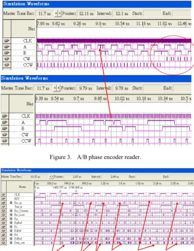
The A/B phase encoder reader is shown in Figure 3. The glitches have been filtered and the noises do not show on the CCW signal. In the upper figure, it shows the original signals and the lower figure shows the zoom in signals. Finally, the PID controller adjusts the control output has been shown in Figure 4.

Figure 2. The PWM Generator.

Figure 3. A/B phase encoder reader.

The Tuning Trend

Figure 4. The PID Controller tuning trend.

The Matlab simulation results are shown in Figure 5 In Figure 5, the position command and division command are given as P=3321 and n= 8, respectively. The total interpolating sections of the T-type velocity curve is twenty- four, and the interpolating time of the acceleration segment, the deceleration segment and the constant velocity segment are equal. The Quartus II simulation is under the position command P=320 and the division number n=2. The simulation result is shown in Figure 6.

0 5 10 15 20 25 30 35

0 1000 2000 3000 4000

0 5 10 15 20 25 30 35

0 50 100 150

Figure 5. T-type velocity curve simulation result, P=3321 and N=8.

(5)

Figure 6. The FPGA simulation result of a T-type velocity curve chip with P=320, n=2.

IV. HANDS-ONIMPLEMENTATIONAND EXPERIMENTS

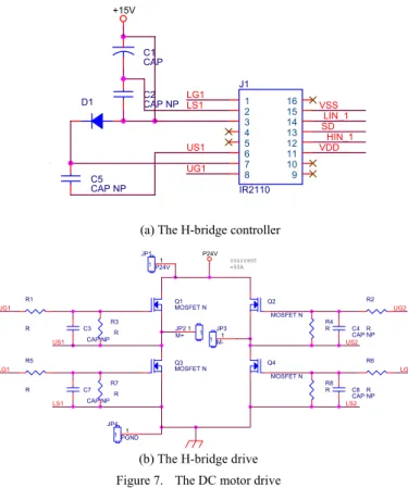
The DC motor drive has been implemented by two IR2110.

It is shown in Figure 7 with half control circuit, for example.

The drive works under 55V DC power and 50 A current. The issue of the dead time protection is important. The controller is implemented by the FPGA, and the dead time may use the internal timer to control the on-time of the PWM signals.

+15V

LIN_1 HIN_1 US1

LS1 LG1

VSS

UG1

VDD SD J1

IR2110 1 2 34 5 67 8

16 15 1413 12 1110 C5 9

CAP NP

D1 C2

CAP NP C1CAP

(a) The H-bridge controller

P24V

UG2

LG2 UG1

LG1 US1

LS1 LS2

US2 R3

C3 R CAP NP R1

R

R7 C7 R

CAP NP R5

R

JP4 PGND 1 1

JP1 P24V1 1

JP2 M+

1 1 JP3

M-1 1 Q1 MOSFET N

Q3MOSFET N

Q2 MOSFET N

Q4 MOSFET N

R4

R C4

CAP NP R2

R

R8

R C8

CAP NP R6

R courrent

=50A

(b) The H-bridge drive Figure 7. The DC motor drive

In the study, there are two stepping motor for driving the head of the mobile robot. The TA8435H is introduced to implement the stepping motor drive. The design circuit is shown in Figure 8.

24V

5V

/RESET /ENABLE CW -CCW

M1 REF_IN /MO

PHASE-NB PHASE-B PHASE-NA PHASE-A CK1 CK2 M2

24V5V U1

TA8435H S-GND1 RESET 2 ENABLE3 OSC4 CW /CCW5 CK26 CK17 M18 M29 REF IN10

MO11 NC12 VCC 13 NC14 VMB15 PHASE-B16 P-GND-B17 NFB18 PHASE-B19 PHASE-A20 NFA21 P-GND-A22 PHASE-A23 VMA24 NC25

C1 0.0033uF

R10 0.8/2W R9 0.8/2W

0.2uF/CERAMICC3 +220uF/35VC4

C2 0.2uF/CERAMIC

R1 4.7k R2 4.7k R3 4.7k R4 4.7k

S1 SW DIP-8

1234 5678

16151413 1211109

R5 4.7kR6

4.7kR7 4.7kR8

4.7k

J3

CON4 1 23 4

J1

CON2 1 2

J2

CON3 12 3

Figure 8. Stepper Motor Drive Circuit

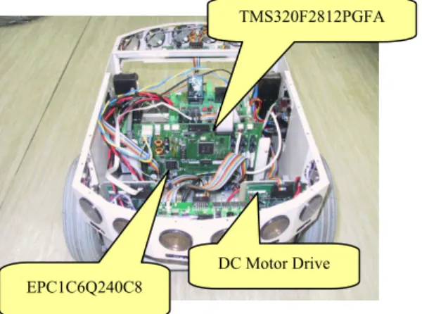
The motion control algorithms have been implemented on an Altera FPGA, and the DC motor drive has been implemented by printed-circuit technology. Both modules have been integrated into a mobile system; a simple verification system block diagram is shown in Figure 9. The controller of the UBot mobile robot platform is designed by the TMS320F281 and the EPC1C6Q240C8. The driving system of the UBot robot consists of two DC servo motor and two proposed DC motor drives. The internal assembly of the UBot mobile robot is shown in Figure 10. The master computer remote controls the UBot to localization through the wireless LAN. On the other hand, the experimental humanoid mobile robot includes a wheeled mobile robot platform, a body with 1 DOF arm, and a head with CCD eyes. In this paper, the experiments are tested on this mobile robot, which weight is over 50 Kg, shown in Figure 11. The system experimental result has been shown in Figure 12. In Figure 12-(a), the black asterisks represent the obstacle; red circles represent the obstacle avoidance stage of the mobile robot; the red squares represent the odometry of the mobile robot. From day after day cycling testing of the mobile robot obstacle avoiding algorithms [4-5], it shows that the motion driving module has high reliabilities and excellent stabilities.

FPGA/DSP Board

DC Motor

Drives Mobile Robot Encoder Feedback Obstacle Avoidance Robot

Position/Velocity System Sensors

Commands

Figure 9. A simple verification system block diagram

(6)

Figure 10. The internal assembly of the UBot robot.

Figure 11. UBot and experimental mobile robot.

-100 0 100 200 300 400

-200 -150 -100 -50 0 50 100 150 200

X(cm)

Y(cm) Start

End

(a) Odometry Map

0 20 40 60 80 100 120 140 160 180

-150 -100 -50 0 50 100 150 200 250

robot-vel(mm/s) , robot-theta(0.1°/s)

robot-vel(mm/s) robot-theta(0.1°/s)

(b) Velocity and angular velocity of mobile robot Figure 12. Mobile robot obstacle avoidance experimental result

V. CONCLUSIONS AND FITURE WORKS

In this paper, the motion controller on the FPGA and the motor drives are proposed. There are many functions of the FPGA for the UBot system has not been presented. Those functions include: (1) the sonar sensors/ IR sensors control algorithm, (2) the I2C communication algorithm for compass sensor/gyro sensor, (3) UART implementation code, and (4) general purpose I/O. On the control board of the UBot system, there is a DSP, which is used to design the system level program, uplink communication, and system information integration. On the other hand, the complex path planning and generating interpolation data of the motion trajectory are served by the DSP. In the near future, we would minimize the control board for mini-robot. That means the hardware footprint should be limited by the new criteria. The FPGA will take more responsibilities to involve more control algorithms and sensor control interfaces. Based on the title of the paper, we show a whole system design concept and the major function algorithms of a motion controller.

ACKNOWLEDGMENT

The authors gratefully acknowledge the generous assistance of supporting engineers, Sao Chun Lu and the team members, who served the assembling and testing jobs of the system.

REFERENCES

[1] “Modern control Engineering” By Katsuhiko Ogata, Prentice –Hall, INC.

[2] “Computer Control of Manutacruring systems”, by Yoram Koren, McGraw-Hill Book Co.

[3] http://www.engin.umich.edu/group/ctm/PID/PID.html

[4] Z. Guanghua, D. Luhua, and W. Wei, "A Method for Robustness Improvement of Robot Obstacle Avoidance Algorithm," in Robotics and Biomimetics, 2006. ROBIO '06. IEEE International Conference on, 2006, pp. 115-119.

[5] G. Mester, "Obstacle Avoidance of Mobile Robots in Unknown Environments," in Intelligent Systems and Informatics, 2007. SISY 2007. 5th International Symposium on, 2007, pp. 123-127

[6] Carrica, D., Funes, M.A., and Gonzalez, S.A., “Novel stepper motor controller based on FPGA hardware implementation,” IEEE/ASME Transactions on Mechatronics, Vol. 8, Issue 1, March 2003, pp. 120 – 124.

[7] Meckl, P.H.; Arestides, P.B, “Optimized s-curve motion profiles for minimum residual vibration,” American Control Conference, 1998. 24- 26 June 1998, Volume 5, pp. 2627 – 2631.

[8] Nippon pulse PCL5022 manual.

[9] Robot company’s MCX314 manual.

EPC1C6Q240C8

TMS320F2812PGFA

DC Motor Drive