Evolutionary Algorithms for Hard Combinatorial Optimization Problems

(1)

Chapter 4 Evolutionary Algorithms for Hard Combinatorial Optimization Problems

Since the complexity of the deductive games grows at an exponential rate, it is very difficult to obtain optimal strategy for them when they have higher dimensions, as well as for hard-combinatorial problems with lager sizes. Therefore, evolutionary algorithms [Ben99, Kal03]

were employed to solve deductive games. Very often these algorithms are able to find approximately optimal solutions for these complicated problems within a reasonable time. In this chapter, we will investigate evolutionary algorithms for solving hard-combinatorial problems.

First, we introduce the fundamental concepts of evolutionary algorithms in Section 4.1. Then, in Section 4.2, we apply evolutionary algorithms to solve deductive games. Section 4.3 introduces a state-of-the-art CO problem: minimization of Binary Decision Diagrams (BDDs). Section 4.4 presents the new model, elitism-based evolutionary algorithms (EBEA), to solve BDD minimization problems. The distributed implementation of EBEA, DEBEA, is developed in Section 4.5. Section 4.6 reports some experimental results performed by EBEA and DEBEA.

Section 4.7 contains our conclusions.

(2)

4.1 Evolutionary Algorithms (EAs)

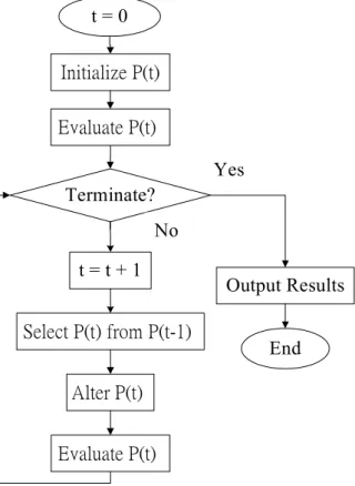
Evolution-based computational approaches have been explored since the early day of computer science [Box57]. The approaches are derivative-free, general-purpose optimization methods based on the concepts of generation-to-generation evolutionary process. Genetic algorithm (GA) [Hol75], based purely on natural selection, is the most popular branch of EA. The characteristic of GA is the notion of emphasizing crossover as the key operation in such system. An important property for these evolution-based search methods is that they maintain a population of potential solutions while other methods process a single point of the search space. Therefore, for a large class of hard combinatorial problems, EAs are robust and able to efficiently find solutions that are approximately optimal. Fig. 4.1 shows the structure of EA.

In Fig. 4.1, P(t) = {ind

1

, ind

2

, ind

3

, …, ind

n

} denotes a population of n individuals of generation t, where n is the size of a population. Each individual represents a potential solution to

Fig. 4.1. The structure of an evolutionary algorithm.

t = 0

Initialize P(t)

Select P(t) from P(t-1)

Alter P(t)

Evaluate P(t) Terminate?

t = t + 1

Output Results

End Evaluate P(t)

Yes

No

(3)

the problem at hand. At each generation, each individual will be evaluated to give some “fitness”.

At select step, a new population P(t+1) is formed by selecting the more fit individuals. Alter step performs some genetic operators, e.g., crossover or mutation operators, to form (possibly more promising) new solutions. This process will be repeated until the termination condition is satisfied.

EAs have been quite successfully applied to optimization problems [Mic99] like wire routing, scheduling, adaptive control, game playing, cognitive modeling, transportation problems, traveling salesman problems, optimal control problems, database query optimization, etc. More recently, EAs have become important for the applications such as machine learning [Mit97] and data mining [Blu03]. Furthermore, EAs also play an important role in parallel computing [Wil99]

and Artificial Intelligence [Fer99] [Rus03] communities.

In general, characteristics of EAs include:

EAs can efficiently explore the search space in order to find (near-)optimal solutions.

EAs are easily parallelized and implemented on parallel processing machines.

EAs are a general, not problem-specific, model for various optimization problems.

EAs are less likely to get trapped in local optimal.

In the following sections, we will take advantage of the characteristics and apply EAs to solve deductive games and hard-combinatorial problems with lager sizes.

4.2 Solving Deductive Games Using EAs

With excellent ability to solve hard CO problems, EAs have been applied to solve deductive games in many published results [Ben99, Ber96, Kal03, Mer99]. In this study, we have also implemented a simple EA to solve deductive games. A simple heuristic function was given to measure “fitness” of individuals, as the following formula:

Score = (2*A+B)

where A = number of “direct hits” and B = number of “indirect hits”.

(4)

Each individual, encoded as an integer string, represents a potential guess in the game. To calculated fitness for an individual, it is evaluated against all previous guesses as if the previous guess is a secret code and the individual is a guess to that code. The individuals with higher scores will survive to the next generation. One-point crossover [Hol75], and no mutation, operators are used in the EA. To compare performances of variant algorithms, we have further implemented two algorithms, namely, first-fit and randomized algorithms, in addition to the genetic algorithm. The first-fit algorithm keeps a set of remaining candidates, which are compatible with the responses given so far, and chooses the first remaining candidates to be the next guess. The randomized algorithm is almost the same as the first-fit algorithm except that it randomly chooses a remaining candidate as the next guess.

This series of experiments are performed for Mastermind games with different dimensions, named 4×6, 4×10, and 4×12. The three algorithms for the three games mentioned above are considered. For each of 9 (33) combinations, 1000 independent runs have been realized. For each independent run, GA performs 5 generations and 300 individuals in a population. The average runtime and number of guesses required for each combination are given in Figs. 4.2(a)* and 4.2(b), respectively. In general, the empirical results can be summarized as follows:

(a) (b)

Fig. 4.2. (a) The run time for Mastermind games with different dimensions. (b) The numbers of guesses required for Mastermind games with different dimensions.

Run time (sec)

0 10 20 30 40 50 60 70

4*6 4*10 4*12

First-fit Randomized GA

Number of guesses

0 1 2 3 4 5 6 7 8 9

4*6 4*10 4*12

First-fit Randomized GA

(5)

The randomized algorithm achieves better results than the first-fit algorithm.

The genetic algorithm achieves best results although the run time is longer (but still much shorter than that for the deterministic algorithms employed in Chapter 3).

The genetic algorithm can not only effortlessly solve games with different sizes but also efficiently obtain “pretty good” results. For the example of 4×6 Mastermind game, the average numbers of guesses required for the genetic algorithm is 4.61, which is not too far to 4.34 for the optimal strategy [Koy93].

4.3 Binary Decision Diagrams (BDD)

In this section, we will introduce a popular CO problem: minimization of BDD, which is NP-complete. Some fundamental concepts will be presented, including BDD representation for Boolean functions, properties of BDD, reduction rules for BDD, BDD minimization problems, and heuristic algorithms for BDD minimization.

4.3.1 BDD representation

A Binary Decision Diagram represents a Boolean function as a rooted, directed acyclic graph.

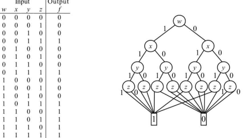
Fig. 4.3 illustrates both truth table and BDD representation of a Boolean function f (w, x, y, z) = wx + yz. Initially, the graph is a binary tree.

Fig. 4.3. Truth table and BDD representation of the Boolean function f (w, x, y, z) = wx + yz.

Input Output

w x y z f

0 0 0 0 0

0 0 0 1 0

0 0 1 0 0

0 0 1 1 1

0 1 0 0 0

0 1 0 1 0

0 1 1 0 0

0 1 1 1 1

1 0 0 0 0

1 0 0 1 0

1 0 1 0 0

1 0 1 1 1

1 1 0 0 1

1 1 0 1 1

1 1 1 0 1

1 1 1 1 1

1 0

0 1

1 0 1

1

0

0 y

1 0 1 0 1 0

1 0 1 0

x x

y y y

z z z z z z z z

w

(6)

The BDD discussed in this study means ordered BDD, which imposes a total ordering ‘<’

over the set of variables and requires that, for any two nodes u and v in any path, their respective variables must be in the same order. Fig. 4.3 shows an example of variables ordered with w < x <

y < z.

4.3.2. Reduction Rules

Since the efficiency of BDD depends on the number of nodes, a BDD should first be reduced before it is manipulated. The following two reduction rules give a canonical form of BDD to a Boolean function under a fixed variable ordering [Bry86].

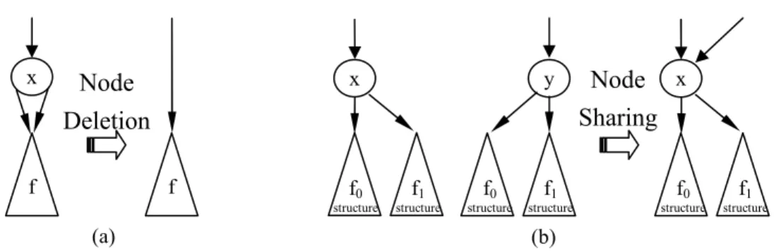
(a) Node deletion rule: We can delete a node x if its two-child links point to the same node, as shown in Fig. 4.4(a).

(b) Node sharing rule: We can merge two (or more) nodes x and y if each of their two child links point to a subtree with the same structure, as shown in Fig. 4.4(b).

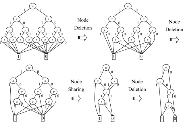
We now apply the two reduction rules to the BDD shown in Fig. 4.3. Fig. 4.5 illustrates the reduction process step by step.

The variable order can be arranged arbitrarily and is very critical for the efficiency of the follow-up manipulation. Fig. 4.6 shows the effect of different variable orderings. Both Figs. 4.6(a) and 4.6(b) represent the function f = x

1

x

2

+ x

3

x

4

+ x

5

x

6

. In Fig. 4.6(a) the variable ordering with x

1

< x

2

< x

3

< x

4

< x

5

< x

6

yields a BDD with a size (the number of nodes) of O(n). (The number of variables is denoted as n.) On the other hand, in Fig. 4.6(b), the variable ordering with x

1

< x

3

<

x

5

< x

2

< x

4

< x

6

yields a BDD with a size of O(2

ⁿ

).

f x

(a) f

y x

Node Deletion

Node Sharing

(b) x

f0 structure f1

structure f0 structure f1

structure f0

structure f1 structure

Fig. 4.4. The reduction rules for BDDs. (a) Node deletion. (b) Node sharing.

(7)

4.3.3 Minimization of BDD

Binary Decision Diagrams (BDDs) [Bra84, Bry86, Gun99, Keb92] are the most popular data structures used for handling Boolean functions because of their efficiency. By using BDDs, Boolean functions can be manipulated in polynomial time/space (in term of the number of nodes of the graph) [Bry92].

Node Deletion

0 0 0 0

1 0

0 1

1 0 1

1

0 y

1 1 1

x x

y y y

z z z

1 0

1 0 w

1 0

0 1

1 0 1

1

0

0 y

1 0 1 0 1 0

1 0 1 0

x x

y y y

z z z z z z z z

w

1 0

0 1

1 0

1 x

y

1 z 0 0

Node Deletion Node

Sharing

0 0 0

1 0

0 1

1 0 1 0

1 1 1

x x

y y y

z z z

1 0

1 0 w

0

1 0

0 1

1 0 1 0

1

x x

y 1z 0 w

Fig. 4.5. The BDD reduction of the Boolean function f (w, x, y, z) = wx + yz.

x1

x2

x3

x4

x6

0 1

x5

x1

x4

x3

x5 x5

x2 x2

x3

x5 x5

x2 x2

x4

x6

1 0

(a) (b)

Fig. 4.6. Different BDD representations for the function f = x

1

x

2

+ x

3

x

4

+ x

5

x

6

.

(8)

Though BDDs are excellent representations for Boolean functions, their sizes are sensitive to the order of the input variables and they may vary from linear to exponential. Finding the optimal variable ordering which results in minimizing the size of a BDD is known to be NP-complete [Bol96a], so that most minimization algorithms are only applicable to small-sized functions [Dre00, Dre01, Ish91, Jeo93]. Also, both the number of variables and their order affect the performance of a minimization algorithm, i.e., changing the initial variable ordering of the same function may prevent an algorithm from finding the exact minimum. This nature of BDDs makes the feature of a minimization algorithm unable to be properly measured. To reduce run time and space requirement, Drechsler et al. [Dre01b] proposed a statistical approach for constructing BDDs.

For BDD-based technology, quality is a very important issue, since a small improvement in the number of nodes often simplifies the follow-up problem tremendously. Various techniques for BDD minimization have been developed in the past decade [Bol96b, Dre01, Ish91, Jeo93, Mol94, Rud93, Sch99, Pan95]. These enable their minimization algorithms to determine the best variable ordering of functions with 7 variables [Fri90], and with 64 variables (for those with partially symmetric functions) [Dre00]. A randomized algorithm has been applied to the problem [Lin01] and has obtained the best size for some benchmark circuits with less than 500 variables.

Recently, scatter search is used to minimize the BDD size [Hun02], which shows robust results compared with the Exact algorithm [Dre00] and other heuristics [Dre01]. However, among 30 benchmark circuits that are manageable by the Exact algorithm, it still could not find the optimal variable orders for five of them.

The BDD minimization problem is to choose a variable ordering leading to minimal BDD size. The Exact minimization problem [Dre00] is to find the optimal variable ordering leading to the smallest BDD. Since it is NP-hard to find the exact minimum, no heuristic algorithms [Dre01]

can find the best variable ordering when n is large. The most promising methods for BDD

minimization are based on dynamic variable ordering (DVO) [Rud93], i.e., the BDD size is

(9)

improved using exchanges of neighboring variables. One application of DVO, Sifting [Rud93], is the most popular heuristics for BDD minimization.

4.3.4 Heuristic Algorithms for BDD Minimization

In this study, we will make use of the problem-specific heuristics, Sifting, and the basic operation of DVO, exchange of adjacent variables (EAV). We now briefly describe these algorithms and analyze the computational complexities.

A. Exchange of adjacent variables (EAV). The exchange is performed very quickly since only partial edges should be redirected within these levels. Hence, the BDD doesn’t need to be completely reconstructed. The resultant BDD would be efficiently minimized if the BDD size becomes smaller after performing EAV. To simplify the analysis, we extend EAV to include the operation of computing BDD size after EAV. In this study, we consider EAV as an elementary operation; in addition, we denote the time complexity of the elementary operation as T

EAV

.

B. Sifting. The sifting algorithm successively considers each variable of a given BDD. At each step, it chooses a variable v

max

and finds the best position of the variable, assuming that the relative order of all other variables remains the same. The variable with the maximum level size is chosen to be variable v

max

. For example, in Fig. 4.6(b), variables x

5

and x

2

both have size 4 in their respective levels. Either x

5

or x

2

could be chosen as v

max

. To find the best position, at least O(n) EAVs should be performed. Since there are n variables for an individual, the time complexity of sifting operation is T

sifting

= O(n

²

)*T

EAV

.

4.4 Elitism-Based Evolutionary Algorithm (EBEA)

The fundamental idea of the elitism-based evolutionary algorithm (EBEA) is that individuals in a

population always have aggressive tendencies towards becoming elites and that only the fittest

individuals in a population are chosen for reproduction. Similar idea has been employed in

previous studies the CHC model [Esh91] and family competition models [Cul93, Thi94,

Yan00]. All of these models use enlarged sample space and deterministic sampling mechanism,

i.e., selecting the best individuals from parents and offspring to form the next generation.

(10)

EBEA differs from all previous models in the following two important features. One is the termination criterion, called stable function, which provides information to judge the degree of convergence for a population. The other is the effective ad hoc operators, called SteepestEAV and Sifting operators in the genetic engineering phase. Besides, EBEA employs a global competition mechanism, in which the best individuals out of the union of parents and offspring form the next generation. The mechanism is similar to CHC algorithm but not family competition models, which use local competition, i.e., each competition takes place within a family. The family members may consist of two parents and two children [Cul93, Thi94] or consist of one parent and L children [Yan00]. Furthermore, EBEA does not perform any mutation in the main evolutionary loop, which also distinguishes it from family competition models but not CHC.

!

,

Fig. 4.7. The flowchart of EBEA.

(11)

In this section, we propose a stable function approach for the EBEA, which provides information to judge the degree of convergence for a population. This not only helps to choose a termination criterion for achieving the speed and quality requirements of a system, but also reduces the run time of redundant generations if the system almost has no chance obtaining superior results. Fig. 4.7 illustrates the flowchart of EBEA, whose details are described in the following subsections.

4.4.1 Representation, Initialization and Evaluation

Each individual in EBEA is represented by an integer string of length n, which stands for a variable ordering for a benchmark circuit with n input variables. All n! permutations of the variable orders are feasible solutions. The representation and related operators has been well studied for solving the Traveling Salesman Problem [Fog88, Fog90, Fog93, Gol85, Oli87, Whi89] as well as for some combinatorial optimization problems.

The initial population is chosen at random. The size of the initial population is denoted by popsize and is fixed during all generations. Since the goal of this research is BDD size minimization, we evaluate individuals by their resultant BDD size.

4.4.2 Operators

Unlike other evolutional algorithms (EAs), as the name “elitism-based evolutional algorithms”

shows, the operators of our EBEA have an aggressive property to let the individuals become elites. We describe the operators in detail as follows:

A. Selection. Enlarged sampling space and deterministic sampling strategy are used; that is, EBEA selects the best popsize individuals from a pool, including not only the offspring but also the old individuals, to produce the next generation.

B. Crossover. The two-point crossover, order crossover OX [Dav85], is used, whose positions

are selected randomly. In EBEA, the crossover operator reserves at least an n/5 proportion of the

chromosome to guarantee “excellent heredity factors” passed on to the next generation. To keep

(12)

the proportion intact, no mutation is used in the main evolutionary loop in EBEA.

We have also tried to use other kinds of crossover operators ER [Whi89], CX [Oli87], and PMX [Gol85] and added mutation operators IVM [Fog88] and ISM [Fog90, Fog93] to EBEA.

However, they often did not improve the results obtained. In contrast, the quality of solutions sometimes decreased. Hence we only apply OX operator in our system.

C. Operators in the genetic engineering phase. In this phase, EBEA changes the genetic structure of individuals in order to make them stronger or more suitable for achieving the goal, i.e., BDD minimization. This is the crux of EBEA and its most time-consuming phase. We take advantage of state-of-the-art heuristics specifically tailored to BDD minimization, namely Sifting.

Furthermore, we design an efficient operator, SteepestEAV, cooperating with Sifting in order to find advanced results more efficiently. In the genetic engineering phase of EBEA, we perform SteepestEAV after Sifting to achieve more superior results. The Sifting algorithm was described in Section 4.2 and has a time complexity of O(n

²

)*T

EAV

. We now describe SteepestEAV and analyze its time complexity.

SteepestEAV. A sketch of SteepestEAV algorithm is given in Fig. 4.8. In the first step, we

perform EAV n-1 times and keep a gain, i.e., the differences in size before and after EAV, for

each adjacent levels (i and i+1) in the array Gain[0~n-1]. If any element of the array contains

positive values, then the BDD size can be improved (i.e., become smaller) after doing the

corresponding EAV. In the second step, we repeatedly perform the EAV with the largest gain to

improve the BDD. After performing each of the EAVs, we have to modify two elements of the

Gain array to reflect the variable ordering change due to the EAV operation. Thus, three

additional EAVs have to be done for each improvement. Therefore, the complexity of

SteepestEAV is T

SteepestEAV

= O(n+3i)*T

EAV

, where i is the number of improvements in the

SteepestEAV operation.

(13)

SteepestEAV(CurrentBDD) { Integer Gain[n] ;

Integer OriginalSize = size_of (CurrentBDD);

Integer NewSize;

for ( i = 0 ; i < n - 1 ; i++ )

{ NewBDD = EAV(CurrentBDD, i, i + 1) ; NewSize = size_of (NewBDD) ;

Gain[i] = OriginalSize - NewSize ; while ("x # Gain[x]>0)) }

{ ^k⁼^max

{

^{x Gain x}^{[ ] 0}^>

}

^;

CurrentBDD = EAV(CurrentBDD, k, k + 1) ; Gain[k] = 0 ;

Update Gain[k - 1] ; Update Gain[k + 1] ; }

}

// the gain for each EAV

// perform variable exchange between levels i and i+1

// compute BDD size for NewBDD

// compute the gain due to the variable exchange between levels i and i+1 and save it in Gain[i]

// do the EAV until no gain for all adjacent variables exchange

// the EAV with largest gain first

// perform variable exchange between levels k and k+1

// reset Gain[k] to 0

// perform variable exchange between levels k-1 and k and update Gain[k-1]

// perform variable exchange between levels k+1 and k+2 and update the Gain[k+1]

Fig. 4.8. A sketch of the SteepestEAV algorithm.

According to the above analysis, the complexity for Sifting and SteepestEAV is (O(n

²

) + O(n+3i))*T

EAV

. Although the run time for the combination is slightly longer than O(n

²

)*T

EAV

for Sifting, the experimental results show that it has an excellent ability to discover advanced results.

Example 4.1. We have tested 103 benchmark circuits in the LGSynth91. Experimental results show that 31 circuits can obtain more superior results by using the proposed operator compared to Sifting. Notice that, the superior results cannot be easily discovered by another independent run with the Sifting method. Moreover, our approach finds the exact minimization solution for circuit cm163a, the results of which cannot be found even for convergent sifting [Som01], a heuristic algorithm that iteratively does Sifting until no further improvement is obtained.

4.4.3 Termination Criteria

Conventional EAs [Dre97] for BDD minimization usually do not stop until the current best result

does not change after hundreds or thousands of additional generations. Such a long time for the

redundant generations is not acceptable by our EBEA since the strong operators for the genetic

engineering phase are more time-consuming than conventional EAs. In contrast, we propose an

(14)

effective termination criterion for EBEA, which supervises the states of all individuals of a generation instead of just measuring the current best result. To be more precise, we develop our termination criteria as follows.

Let P={p

0

, p

1

, p

2

, …, p

popsize-1

}, C={c

0

, c

1

, c

2

, …, c

popsize-1

}, and Q={q

0

, q

1

, q

2

, …, q

popsize-1

} be the sets of sizes for individuals of the parent, the children, and the new population, respectively. Fig. 4.9 shows the general structure of EBEA and illustrates the relation of these sets in EBEA. Here we assume that p

0

p

1

p

2

… p

popsize-1

and q

0

q

1

q

2

… q

popsize-1

. The set of differences is defined as D = {d

i

| d

i

= p

i

-q

i

, 0 i popsize-1}. In EBEA the selection strategy, which includes the techniques of enlarged sampling space and deterministic sampling, makes all the elements in D be nonnegative integers, as proven in Property 4.1. This property is important for developing the termination criteria for EBEA.

Property 4.1. ' d

i

D, d

i

N, i.e., all the elements in the set belong to {0,1,2,3,…}.

Proof. Let sequence S, s

0

s

1

s

2

… s

2*popsize-1

, be the result of sorting all the elements in sets P and C. We have s

i

= q

i

for 0 i popsize-1, since the selection rule, enlarged sampling space, is

Fig. 4.9. The general structure of EBEA showing the relation of three populations, parents, children, and new population. The items, p

i

, c

i

, and q

i

, 0 i popsize-1, inside the rectangles refer to the BDD sizes for individuals, i.e., the elements in sets P, C, and Q, respectively.

NewPopulation Sort

Stable(α,κ)=1?

P aren ts ← N e wP o p u latio n

Stop Parents

OX OX

OX ...

Crossover Children

S i f t i n g & S t e e p e s t E AV S i f t i n g & S t e e p e s t E AV

S i f t i n g & S t e e p e s t E AV ..

.

GeneticEngineering

Selection

Yes No

p0

p1

p2

p3

ppopsize-1

.. .

c0

c1

c2

c3

cpopsize-1

. . .

q0

q1

q2

q3

qpopsize-1

. . .

Union

(15)

used in EBEA. Accordingly, s

i

p

i

and hence q

i

p

i

for all 0 i popsize-1. By definition, d

i

=

p

i

-q

i

0. The result of this property follows. g

From Property 4.1, we have the following observations.

Observation 4.1. If d

0

= 0, then the best size of the population has no change in this generation.

In addition, the more elements in set D that equal zero, the more stable the population, i.e., with a lower probability of obtaining better results. In the extreme case, if all elements in set D are equal to zero, then we call the population stagnant, i.e., no individual obtains a better result in this generation.

Observation 4.2. The effect of d

i

on the final result of a population decreases as i increases. For example, if d

0

> 0, then the current best results have improved during this evolution, and the current best individual, denoted by ind

0

, is still not stable; in addition, any improvement of ind

0

in the next evolution will obtain more superior results. On the other hand, an improvement of d

k

from an unstable individual ind

k

should be large enough so as to improve the best results since its resultant BDD has to be smaller than those of ind

0

, ind

1

, …, ind

k-1

, whose results are all smaller than that of ind

k

in the preceding generation.

Accordingly, the termination criterion of EBEA is determined by the following formula:

Stable function:

stable( , !) = < ⁺ ⁺

=

+

. ,

0

, R , Z where , ,

1 ¹

0

) 1 ( log₂

otherwise d_i

popsize i

i

! !

That is, EBEA will stop if the value of the stable function is equal to 1. Notice that we give

different weights to d

i

according to the effect on the final result. In addition, a problem specific

parameter is used, which depends on the range of the problem in hand; for example, we

choose =5 in the BDD minimization problem. Now, we derive the properties of the stable

function and give two examples to show how it works in Property 4.2 and Examples 4.2 and 4.3.

(16)

Property 4.2. If ! =

^-k

and stable( ,

^-k

) = 1, k N, then the set of differences D satisfies all the following constraints.

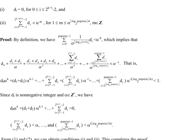
(i) d

i

= 0, for 0 i 2

^k+1

-2, and

(ii) <

= + +

+ 2 2

1 2 i

i m 1 m k

m

k

d , for 1 m

^log2popsize -k

, m Z.

Proof: By definition, we have

^popsize ¹ _i

0

i log1(i 1) d

= 2 +

<

^-k

, which implies that

. ...

...

d

2 log2 1

log 1

2 2

2 1 2 2

6 5 4 3 2 1 0

k popsize popsize

i

i k

i

i popsize

k

d d d

d d d d

d ₌ ₌

<

+ + +

+ + + + +

+ +

+

That is,

d

0 k

+(d

1

+d

2

)

^k-1

+…+

= + 2 2

1 2

i i

1 k

k

d +(

= +

+ 2 2

1 2

i i

2 k

1

k

d )

^-1

+…+(

=

1 popsize 2

i i

popsize

log2

d )

^{-( log}2popsize -k)

< 1.

Since d

i

is nonnegative integer and Z

⁺

, we have d

0 k

+(d

1

+d

2

)

^k-1

+…+

= + 2 2

1 2

i i

1 k

k

d =0, (1)

(

= +

+ 2 2

1 2

i i

2 k

1

k

d ) < , …, and (

=

1 popsize 2 i

popsize i

log2

d ) <

^{( log}2popsize -k)

. (2) From (1) and (2), we can obtain conditions (i) and (ii). This completes the proof. g

150 160 170 180

0 1 2 3 4 5 6 7 8 9

the k-th individual BDD size

Gen1 Gen2 Gen3

Fig. 4.10. The resultant BDD sizes for individuals in three successive generations for the

benchmark circuit alu2. The sets of differences for generations 2 and 3 are D

2

=

{1,3,3,4,1,7,7,12,13,24} and D

3

={0,1,1,0,3,3,3,3,4,4}, respectively.

(17)

Example 4.2. From Property 4.2, if stable( ,1) is chosen, then the termination criterion for EBEA will be (i) d

0

=0, and (ii) d

1

+d

2

< , d

3

+d

4

+d

5

+d

6

<

²

, …,

=

+

2 <

2 1 2

1 k

i k

k

di

, …, and

= 1 2^log² popsize i

i

popsize

d

<

^log²^popsize

. For example, Fig. 4.10 illustrates the resultant BDD sizes for individuals

in three successive generations for the benchmark circuit alu2. Observe that the sets of differences for generations 2 and 3 are D

2

={1, 3, 3, 4, 1, 7, 7, 12, 13, 24} and D

3

={0, 1, 1, 0, 3, 3, 3, 3, 4, 4}, respectively. If stable(5,1)=1 is chosen, then EBEA stops at generation 3 and outputs the best size 154 since D

3

satisfies the termination criterion. g Example 4.3. If stable( ,1/ ) is chosen for an EBEA, then the termination criterion would be more strict, that is,

^popsize ¹ _i

0

i log1(i 1) d

= 2 +

<1/ , which implies that it should also satisfy all the following conditions: (i) d

0

=d

1

=d

2

=0, (ii) d

3

+d

4

+d

5

+d

6

< , …,

⁺

<

= 1 2 2

1 2

1 k

i k

k

d

i

, …, and

=

1 popsize 2 i

popsize i

log2

d <

^log²^{popsize -1}

. g

We now summarize the important features of the proposed termination strategy.

It can supervise not only the overall status of a population, but also the most important factor, i.e., whether d

i

is equal to zero or not, for smaller i.

It is very easy to implement since the stable function deals only with differences of the evaluated values, e.g., the BDD sizes, in each generation.

It can be applied to any optimization problem if the selection strategy, which includes the techniques of enlarged sampling space and deterministic sampling, is used in the EA.

Both computation and space requirements are only O(popsize). In implementation, we keep

just an extra array with popsize elements to memorize the evaluated values for individuals of

the preceding generation, and only additional O(popsize) operations are required to evaluate

the function.

(18)

In Section 4.5, experimental results show that EBEA is feasible and effective for the BDD minimization problem, although it places more emphasis on local exploitation rather than global exploration. The following key features make EBEA robust for BDD minimization.

The problem-specific heuristic, Sifting, is effective for finding locally optimal solutions (variable orderings).

With the help of the additional SteepestEAV, EBEA can efficiently find further minimized solutions if any of them can be produced by an additional EAV. Notice that the results cannot be easily discovered by another independent run with the Sifting method.

EBEA reduces the run time for redundant generations, since the termination strategy is able to supervise the degree of convergence.

EBEA not only enforces “heredity factors of elites” passing on to the generations of offspring, but also efficiently explores the most promising area to obtain minimized results.

4.5 Distributed Model of EBEA (DEBEA)

In this section, we present the distributed model of EBEA, DEBEA, which is developed by an

elaborate cooperation of components’ EBEA. We have implemented DEBEA on a dedicated PC

cluster which is located at the Graduate Institute of Computer Science and Information

Engineering, National Taiwan Normal University. The hardware includes 8 CPUs (AMD Athlon

MP 2200+), 8 RAM boards (each with 2G bytes), and a switch hub (1G bytes/sec communication

rate). In addition, CUDD [Som01] , Linux RedHat 7.3, gcc compiler, and MPICH are installed on

the PC cluster. MPICH is a portable implementation of MPI, a standard for message-passing

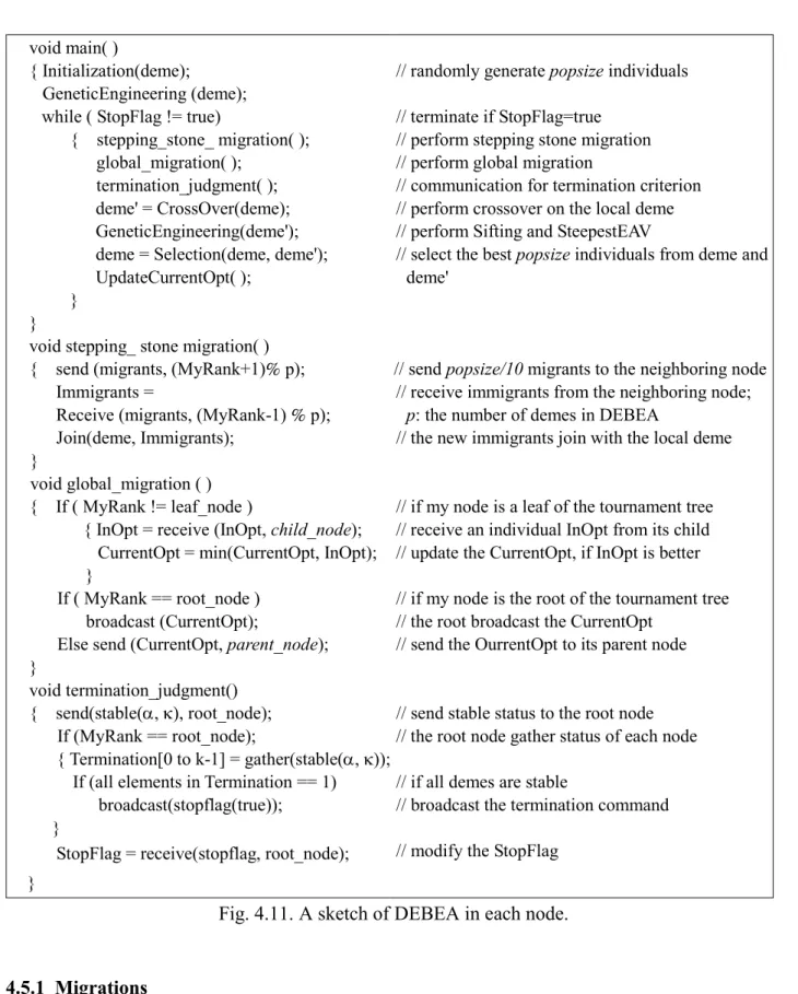
libraries for parallel processing. The sketch of DEBEA is shown in Fig. 4.11. We first introduce

the migrations employed in DEBEA. Then, the termination criteria of DEBEA are developed.

(19)

void main( )

{ Initialization(deme);

GeneticEngineering (deme);

while ( StopFlag != true) { stepping_stone_ migration( );

global_migration( );

termination_judgment( );

deme' = CrossOver(deme);

GeneticEngineering(deme');

deme = Selection(deme, deme');

UpdateCurrentOpt( );

} }

void stepping_ stone migration( )

{ send (migrants, (MyRank+1)%p);

Immigrants =

Receive (migrants, (MyRank-1) %p);

Join(deme, Immigrants);

}

void global_migration ( )

{ If ( MyRank != leaf_node )

{ InOpt = receive (InOpt, child_node);

CurrentOpt = min(CurrentOpt, InOpt);

}

If ( MyRank == root_node ) broadcast (CurrentOpt);

Else send (CurrentOpt, parent_node);

}

void termination_judgment() { send(stable( , !), root_node);

If (MyRank == root_node);

{ Termination[0 to k-1] = gather(stable( , !));

If (all elements in Termination == 1)

broadcast(stopflag(true));

}

StopFlag = receive(stopflag, root_node);

}

// randomly generate popsize individuals // terminate if StopFlag=true

// perform stepping stone migration // perform global migration

// communication for termination criterion // perform crossover on the local deme // perform Sifting and SteepestEAV

// select the best popsize individuals from deme and deme'

// send popsize/10 migrants to the neighboring node // receive immigrants from the neighboring node;

p: the number of demes in DEBEA

// the new immigrants join with the local deme

// if my node is a leaf of the tournament tree // receive an individual InOpt from its child // update the CurrentOpt, if InOpt is better // if my node is the root of the tournament tree // the root broadcast the CurrentOpt

// send the OurrentOpt to its parent node

// send stable status to the root node // the root node gather status of each node // if all demes are stable

// broadcast the termination command // modify the StopFlag

Fig. 4.11. A sketch of DEBEA in each node.

4.5.1 Migrations

In DEBEA, each CPU node runs an EBEA for a semi-isolated population, called deme. Two

types of migrations are produced for each deme, stepping-stone and global migrations. Both

types of migrations are performed at every generation. A unidirectional ring network structure is

(20)

used in the stepping-stone migration, while both tournament tree and star network structures are used in the global migration. Fig. 4.12(a) illustrates the ring and tournament tree network structures for the migrations in DEBEA.

In the stepping-stone migration, each EBEA randomly selects popsize/10 individuals to migrate to its neighboring node in the ring network. Each node put the immigrations into a pool, which then includes the old individuals, offspring and the immigrations. The EBEA selects the best popsize individuals from among all individuals in the pool for propagation.

The global migration consists of two phases, collecting and broadcasting. In the collecting phase, a tournament tree connection is used in order to balance the load of both computation and communication. DEBEA collects the best individual from the leaves to the root through the tournament tree. Each leaf of the tournament tree sends the best individual in its deme to its parent node. Each internal node receives a migration, compares it with the best of its own population, and then sends the better of them to its parent node. Finally, the root broadcasts the best individual to each node and then the best individual joins the deme in each EBEA.

Fig.4.12. (a) The illustration of ring and tournament tree network structures for the migrations in DEBEA.

(b) The communication for termination criteria in DEBEA.

(a) (b)

P7

P6

P5

P4

P3

P2

P1

Termination StopFlag=false

P0

0 1 1 0 ...

tournament tree ring

P0 P1 P2 P3 P4 P5 P6 P7

P0

P4

P0

P0 P2 P4 P6

(21)

4.5.2 Termination

As shown in Fig. 4.12(b), the termination criteria adopted in DEBEA requires global convergence, i.e., each local EBEA runs independently until all EBEAs of the system are stable.

The stable function introduced in Section 4.4.3 is used as a termination criterion in DEBEA. A root node keeps a termination array to collect the current value of the stable function from each node. If all the values are equal to 1, then the root broadcasts a termination command, StopFlag=true, to all other nodes. If any EBEA receives the command, then it outputs the best solution and stops.

Features of DEABE can be summarized as follows:

All the network configurations employed in DEBEA can be easily and efficiently implemented on the PC cluster.

Asynchronous communications are used for all communications in DEBEA for efficiency.

The total number of messages passed is O(p) for each generation, including migrations and termination judgments, where p is the number of CPU nodes used.

4.6 Experimental Results

In this section we describe the experimental results that have been carried out on a SUN Ultra 1 and a dedicated PC-cluster for EBEA and DEBEA, respectively. The algorithms have been integrated with the CUDD package [Som01a, Som01b]. We perform two series of experiments as described in the following subsections. For EBEA, only two parameters are required in the experiments, namely, the stable function and the population size.

4.6.1 Performance of EBEA

In the first series of experiments, we compare the results of EBEA with those of the latest published BDD minimization algorithms, Scatter search [Hun02] and Exact algorithm [Dre00].

The results are shown in Table 4.1. Our program is implemented in C on a Sun Ultra 1 with 64

Mbytes memory. This is the same machine but with smaller capacity of memory than that used in

(22)

the experiments [Hun02], in which 300 Mbytes memory is used. The data given in the columns Scatter and Exact of Table 4.1 is directly transcribed from their experimental results. For all circuits, popsize is set to be n/4 for the experiments, where n is the number of input variables.

Also, we perform ten independent runs and choose stable(5,1)=1 as the termination criterion.

The columns Min # and Max # show the minimum and maximum results of BDD size among ten runs. The column No. Opt shows the number of runs that yield the optimal result. The two rightmost columns show the average and the maximum run times of our EBEA required for the ten runs.

Table 4.1. EBEA compared with scatter search [Hun02] and exact algorithm [Dre00], where parameter setting for EBEA is: popsize=n/4 and termination criterion is satisfied if stable(5,1)=1.

The columns Min # and Max # show the maximum and minimum results of BDD size among ten runs. The column No. Opt shows the number of runs that obtain the optimal result. The two rightmost columns show the average and the maximum run time of our EBEA required for the ten runs.

Outputs: # of BDD Nodes CPU Run Time (Seconds)

EBEA EBEA Circuit Inputs

Exact Scatter

Min # Max # No. Opt Exact Scatter

Average Max

alu4 14 350 564 350 355 6 163.0 23.30 5.69 8.74

cc 21 46 46 46 46 10 753.3 5.47 4.66 6.47

cm150a 21 33 33 33 33 10 3858.8 10.96 3.20 4.32

cm162a 14 30 30 30 31 9 4.2 4.07 2.88 3.48

cm163a 16 26 26 26 26 10 7.7 3.71 2.34 2.63

cmb 16 28 28 28 28 10 0.1 5.16 1.84 1.88

comp 32 95 103 95 98 9 47605.4 151.64 8.18 9.98

cordic 23 42 42 42 42 10 23.8 14.22 6.23 8.55

cps 24 971 971 971 974 8 46130.4 56.35 17.03 24.96

cu 14 32 32 32 32 10 6.5 3.94 2.27 2.68

i1 25 36 36 36 36 10 198.7 7.48 3.54 3.94

lal 26 67 67 67 67 10 4595.4 8.13 3.97 4.32

mux 21 33 33 33 33 10 3872.7 10.15 3.00 3.10

parity 16 17 17 17 17 10 0.1 7.59 1.73 1.78

pcle 19 42 42 42 42 10 60.1 5.64 2.30 2.76

pm1 16 40 40 40 40 10 3.8 3.38 2.31 2.65

s1488 14 369 384 369 381 4 90.0 15.12 5.67 9.26

s344 24 104 104 104 104 10 11519.2 9.72 6.09 9.97

s349 24 104 104 104 104 10 11546.3 9.84 5.41 7.20

s382 24 119 119 119 121 5 6637.6 9.96 5.70 8.65

s400 24 119 119 119 121 5 6846.8 9.98 6.31 8.66

s444 24 119 119 119 121 6 6934.0 8.30 5.47 8.71

s526 24 113 113 113 113 10 8809.1 11.55 5.70 7.61

s820 23 220 266 220 221 3 17145.3 21.72 6.90 8.96

s832 23 220 274 220 221 5 17953.8 21.11 7.44 9.08

sct 19 48 48 48 48 10 60.6 6.22 3.13 3.66

t481 16 21 21 21 21 10 1.2 4.17 7.02 9.37

tcon 17 25 25 25 25 10 3.7 1.15 1.76 1.81

ttt2 24 107 107 107 108 9 7087.2 11.07 5.37 7.34

vda 17 478 478 478 488 6 641.6 21.87 6.23 8.79

(23)

Although the Exact algorithm can always get the exact minimum size, its run time explodes as the number of input variables increases. Scatter search could not find the optimal variable order in 5 of 30 benchmark circuits that are manageable by the Exact algorithm. On the other hand, EBEA performs more efficiently and effectively for BDD minimization.

We see that EBEA is able to find the optimal variable orders with very high probability. As shown in Table 4.1 for EBEA, all the optimal orders are found in ten runs; Furthermore, among 30 circuits, 19 circuits achieved the optimal order in each of the 10 runs. The remaining 11 circuits can still get the optimal order in some of the 10 runs. For the example of circuit comp, EBEA finds the optimal order, with the optimal size 95 (=Min #), in 9 (=No. Opt) of 10 runs. The only one remaining run finds a nonoptimal size 98 (=Max #), which is still smaller than 103 found by Scatter search.

For run time, EBEA can efficiently find a better solution and can outperform other algorithms in most cases. For tests with popsize=n/4, all the tests are completed within 10 seconds, except for the benchmark cps with 24.96 seconds. For Scatter search, however, its run time for 12 of 30 circuits is longer than 10 seconds. It takes 151.64 seconds for the benchmark comp and 56.35 seconds for the benchmark cps.

To compare the tradeoff between run time and quality, we also change the popsize

parameter to observe the impact in the resultant BDD size. Table 4.2 shows the experimental

results for popsize=n/2. Although it takes about twice the run time, it not only increases the

probability of finding the optimal solution, but also makes the near-optimal solutions close to the

exact one.

(24)

Table 4.2. EBEA compared with scatter search [Hun02] and exact algorithm [Dre00], where parameter setting for EBEA is: popsize=n/2 and termination criterion is satisfied if stable(5,1)=1.

Outputs: # of BDD Nodes CPU Run Time (Seconds)

EBEA EBEA Circuit Inputs

Exact Scatter

Min # Max # No. Opt Exact Scatter

Average Max

alu4 14 350 564 350 355 7 163.0 23.30 11.10 19.90

cc 21 46 46 46 46 10 753.3 5.47 7.03 8.52

cm150a 21 33 33 33 33 10 3858.8 10.96 5.35 7.34

cm162a 14 30 30 30 31 10 4.2 4.07 5.04 5.12

cm163a 16 26 26 26 26 10 7.7 3.71 4.49 4.99

cmb 16 28 28 28 28 10 0.1 5.16 3.41 3.45

comp 32 95 103 95 95 10 47605.4 151.64 15.32 15.55