Multihop Cellular: A New Architecture for Wireless Communications

Multihop Cellular: A New Architecture for Wireless Communications

Ying-Dar Lin and Yu-Ching Hsu Department of Computer and Information Science National Chiao Tung University, Hsinchu, Taiwan

Absmr-This work presents a new arrhttedure, Multihop Cellular Netwok (MCN), for wireless co"unieations. MCN preserves tbe ben- dit of conventional w e h o p cellular netwoIlts (SCN) where the service Mrastrufture is constructed by fixed bases, and it also incorporatfs the flexibility of ad-hoc networks where whless transmissiOn througb mc+

bile stations in multiple hops is allowed. MCN can reduce the requid number of bases or Improve the throughput performance, while limiting path vulnerability encountered in &hoc networks. In addition, MCN and SCN are analyzed, in term of mean hop caunt, hop-by-hop through- put, end-Wend thmughput, and mean number of channels (Le. simul- taneous transmissions) under Merent tre88c l d t i e s and t"i&on ranges. Numerical results demonstrate that throughput of MCN exceeds that of SCN, the former also increases as the transmission range de- creases. Above results can be accounted for by the merent orders, linear and square, at which mean hop count and mean number of channels In- crease, respectlvely.

Kq~wordr- multihop, cellular, ad-hor networks, packet radio, trans- mission range

I. INTRODUCTION

Wireless communications has rapidly evolved in the recent decade. Within this field, voice-oriented services can be cat- egorized as either [l]: (1) high-power, wide-area cellular sys- tems, e.g. A M P S (Advanced Mobile Telephone System) 121 and GSM (Global System for Mobile communications) [3], or (2) low-power, local-area cordless systems, e.g. CT2 (Cordless Telephony) [4] and DECT (Digital European Cordless Tele- phone) 151. Data-oriented services can also be categorized as either [l]: (1) low-speed, wide-area systems, e.g. ARDIS (Ad- vanced Radio Data Information Service) [6] and CDPD (Cel- lular Digital Packet Data) [7], or (2) high-speed, local-area systems, e.g. HIPERLAN (Hi Performance Radio Local Area Network) 181 and IEEE 802.11 193,

However, most services and systems mentioned above are based on the single-hop cellular architecture. Service providers must construct an infrastructure with many fixed bases or ac- cess points to encompass the service area. By doing so, mo- bile stations can access the infrastructure in a single hop. In a densely populated metropolitan area, to support more connec- tions, the area that a single base, i.e. a cell, covers is shrunk and the number of bases increases. This phenomenon unfortu- nately leads to (1) a high cost for building a large number of bases, (2) total throughput limited by the number of cells in an area, and (3) high power consumption of mobile stations hav- ing the same transmission range as bases. Notably, (1) and (2) trade off each other. If a higher throughput in a geographical area is desiml, more bases. i.e. cells, must be constructed in that area.

Another kind of network, commonly referred to as packet radio or ad-hoc networks [lo], [ll]. is available in which no infrastructure or wirelpe backbone is required. In these net- works, packets may be forwarded by other mobile stations to reach their destinations in multiple hops. Second generation packet radio networks. such as W M S (Wireless Adaptive Mobile Information System [121), have began to address the limited bandwidth and QoS(QuaUty of Service) issue. An ad- vantage of these networks is their low cost because no infras- tructure is required, and, therefore, can be deployed immedi- ately. However, these ad-hoc networks appear to be limited to specialized applications. such as battlefields and traveling groups, due to the vulnerability of paths through possibly many mobile stations. However, this vulnerability can be signifi- cantly reduced if the number of wireless hops can be reduced and the station mobility is low.

In this work, we present a new architecture, Multihop Cel- lular Network (MCN) as a viable alternative to the conven- tional Single-hop Cellular Network (SCN) by combining the features of SCN and ad-hoc networks. The implemented pro- totype, where mobile stations run a bridging protocol, shows that MCN is a feasible architecture for wireless LANs [13].

In MCN, mobile stations help to relay packets, which is not allowed in other variant systems of SCN, such as Ricochet net- work [14] and mobile base network [15]. MCN has several merits: (1) the number of bases or the transmission ranges of both mobile stations and base can be reduced, (2) connections are still allowed without base stations. (3) multiple packets can be simultaneously transmitted within a cell of the correspond- ing SCN, and (4) paths are less vulnerable than the ones in ad- hoc networks because the bases can help reduce the wireless hop count.

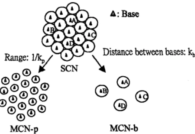
Fig. 1 'shows an SCN and two possible architectures of MCN, MCN-b and MCN-p, as derived from SCN. Although the transmission range adopted in MCN-b is the same as that in SCN. the number of bases is reduced such that the distance be- tween two neighboring bases becomes kt, times of the distance in SCN. Only four base stations, A, B, C. and D in the SCN are necessary in MCN-b. In MCN-p, although the number of bases is not reduced, the transmission ranges of base stations and mobile stations are reduced to l / k p of these adopted in SCN. Thus packets might be forwarded. in both MCN-b and MCN-p, by mobile stations to arrive destinations in multiple hops. Nevertheless, MCN-b can be viewed as a special case

of MCNp if the transmission range and the distance between

0-7803-5880-5/00/$10.00 (c) 2000 IEEE 1273 IEEE INFOCOM 2000

A: Base

Distance between

bases:

kb

Range: 1

MCN-p MCN-b

Fig. 1. Examples of an SCN and two varianls of MCN, MCN-p and MCN-b.

bases in MCN-p are multiplied by kp and kb. respectively. For the example in Fig. 1, the radius of a cell and the distance be- tween bases of MCN-b are twice as long as those of MCN-p, if IC, = kb = 2. This work focuses on MCNp while describing and analyzing the proposed architecture. In addition, MCN-b is analyzed by simple parameter substitution. MCNp is re- ferred to herein as MCN

.

This work focuses mainly on system throughput of SCN and MCN. MCN has its merits and limitations. With respect to its merits, the throughput might be improved, since multi- ple packets can be simultaneously transmitted in a cell of the corresponding SCN. In terms of its limitations, the throughput might be lowered, since packets may have to be sent multiple timcs to arrive at bases or destinations, which consumes more bandwidth. Therefore, the end-to-end throughput of SCN and MCN must be thoroughly analyzed.

The rest of the paper is organized as follows. Section II de- scribes the SCN and MCN architectures. Section III presents the system throughput of SCN and MCN. Section TV summa- rize the numerical results, indicating that the throughput of MCN is better than that of SCN. Hop count and the number of simultaneous channels or transmissions are also studied to explain the results. Finally, conclusion and areas for future re- search are given in section

v.

11. ARCHITECTURE

Single-hop Cellular Networks (SCNs) are cellular networks where bases can be reached by mobile stations in a single- hop, in contrast ^U) Multihop Cellular Networks (MCNs) where bases can not always be reached by mobile stations in a single hop.

Before describing these two architectures, we first define the area reachable by a base in SCN as a cell, which is within a radius of fixed distance, say R. Incidentally, the area of a cell in MCN is also defined as the same area in SCN, which is the area taken care of by a base. Notably, the radius of a cell in MCN is half the distance between two neighboring bases. A

Fig. 2. Multihop routing vs single-hop routing.

pig. 3. Different routing paths of MCN and SCN.

sub-cell in MCN is defined as the area reachable in a single wireless hop by a base or a mobile station. In SCN, the area of a sub-cell is the same as the area of a cell.

A. Single-hop Cellular Network (SCN)

In SCN, base and mobile stations in the same cell are always mutually reachable in a single hop. When having packet? to send, mobile stations always send them to the base within the same cell. If the destination and the source are in the same cell, such as stations 1 and 4 in Fig. 2, the base directly forwards packets to the destination. If the destination is in a different cell, the base forwards them to the base of the cell where the destination resides. The base of the latter cell then forwards packets to the destination in a single hop. Thus, the routing path resembles the dashed lines in Figs. 2 and 3.

B. Multihop Cellular Network (MCN)

The architecture of MCN resembles that of SCN except that bases and mobile stations are not always mutually reachable in a singIe hop. The transmission range of bases and mobile stations is reduced to l / k p of that adopted in SCN. Thus, the area reachable by a base or a mobile station is simply the area of a sub-cell. Similar to ad-hoc network,. a key feature of MCN is that mobile stations can directly communicate with each other if they are mutually reachable, which is not allowed in SCN. This feature leads to multihop routing.

If the source and the destination are in the same cell, other mobile stations can be used to relay packets to the destination, which achieves multihop routing within a cell. If not in the same cell, packets are sent to the base first, probably in multi- ple hops, and then be forwarded to the base of the cell where the destination resides. Packets can then be forwarded to the destination. probably in multiple hops again. within the latter

Q-78Q3-588Q-51QQ1$IO.QO (c) 2000 IEEE 1274 IEEE INFOCOM 2000

TABLE I SUMMARY OF PARAMETERS.

sion since a renewal point

the total packet arrival rate at mobile stations within a cell the packet arrival rate at the base

the probability of successful exchange of WS and CTS

(3.

. Gba Pa Fig. 4. Three stations in a cell transmit at the same time in MCN.

cell.

The solid lines in Figs. 2 and 3 illustrate the above two cases. These figures reveal the different routing paths of MCN and SCN by solid and dashed lines, respectively. The main advantage of MCN is the increased system throughput, a$ an- alyzed in the next section. For example, in Fig. 4, stations 1, 3, and 5 within the same cell can transmit packetfs simultane- ously without interfering with each other; meanwhile, only one packet can be transmitted in the corresponding SCN.

111. MODELING A N D ANALYSIS A. Underlying Assumptions and Definitions

To model the system throughput of SCN and MCN, we first assume that the up-link and down-link in a cell share the same channel for the inter-communication between mobile stations.

For example, if station 2 in Fig. 3 transmits in chl and lis- tens to ch2. station 3 would have to listen to chl and transmit in another channel. Thus, another control channel would be indispensable to process the complicated channel assignment when a mobile station transmits and receives packets in sepa- rate channels, making our analysis intractable. For compari- son, the same assumption is also applied to SCN.

This work ako applies the RTS/@TS (Request To Send / Clear To Send) access method of DCF (Distributed Coordina- tion Function) of E E E 802.1 1 191 MAC (Medium Access Con- trol) protocol to both architectures, while assuming that neigh- boring celk use different channels to avoid conflict. Hence, the need for synchronization is eliminated. Furthermore, station mobility is neglected to reduce the complexity of our analy- sis since the simulation results in 1161 show the small effect of mobility on system throughput.

Once a channel is sensed idle and a time interval DIFS @CF Inter-Frame Space) has elapsed, the time until a data packet is generated at station i. destined for station j in the same cell.

is assumed to be exponentially distributed with rate Xij. Also, Xc is denoted as the rate at which data packets are generated at station i destined for stations outside the cell. Similarly, X,i is the rate at which data packets are generated outside the cell and destined for station i in the cell. The number of stations in the cell i s denoted as N and the radius of the cell is denoted as

I

I packets

I

0-7803-5880-5/00/$10.00 (c) 2000 IEEE 12 75

R. In addition, r , ZRTS, ZCTS. Z P K T , ~ A C K , ~ S X F S and ~ D I F S

are used to denote the maximum propagation delay in one hop, the transmission time of an RTS packet, a CTS packet, a data packet and an acknowledgment packet, a$ well as the time in- terval of SIFS (Short Inter-Frame Space) and DIFS, respec- tively.

Herein, the system throughput is definedusing the same def- inition as 1171, i.e. the number of successful transmissions be- tween successive "renewal points" divided by the length of the time interval between the renewal points, referred to as a re- newal interval. However, the "renewal point" is defined a$ the time point when all stations in a sub-cell simultaneously sense the channel being idle. Thus, the expected length of a renewal interval is defined as

where P8 denotes the probability of successful exchange of RTS and CTS packets, and t i d e represents the expected time until the initiation of the first transmission since a renewal point. Notably, both t i d e and Pa are to be derived.

Our goal is to derive the hop-by-hop throughput and end-to- end throughput in a cell for both S C N and MCN. The hop-by- hop throughput is defined as the number of successful packet transmissions per second in a cell. The end-to-end throughput is defined as the number of successful packet receptions per second in a cell by either the base, if the end destinations are outside the cell, or the end destinations, if they are within the

IEEE INFOCOM 2000

cell, We use table I to summarize the parameters mentioned above.

B. Single-hop Cellular Network System throughput analysis:

steps:

1. Derive tidbe to obtain the renewal interval;

2. Derive the probability of a successful transmission at station i and the base;

3. Derive the throughput of station i and the base; and 4. Derive the hop-by-hop throughput and end-to-end through- put of SCN.

To obtain m q c l e , the packet arrival rate at station i is com- The system throughput of SCN is analyzed in four major

puted as

N

Xi = Xij

+xi,.

(1)

j#i,j=l

Now we denote the total packet arrival rate at mobile sta- tions within a cell by G, which equals

ELl

Xi. Since each packet transmitted from station i to station j is forwarded by the base, the traffic generation rate at the base is given by Gbs =

ELl

^X,i

+

&i,j=l & j . Thus, t - i d e is de- rived as 1/(G,

+

& , ) . since the packet arrival process is Pois- son and a sub-cell equals a cell in SCN. The renewal interval is thus given by

N N

To analyze the probability of successful transmission from station i, at time t, to the base, we first define mean capture area and mean hidden area of station i as AI and A2, respec- tively, in Fig. 5. The capture area of station i is the area within the cell reachable by station i. The hidden area of station i is the capture area of the receiver, i.e. the base station, but is hid- den from station i. For convenience, Al/nRa and A2/7rR2 are denoted as n h (i.e. mean percentage of capture area in a cell) and h (i.e. mean percentage of hidden area in a cell), respectively, where nR2 represents the area of the cell. Since P(the distance between the base and station i = a) =

9,

A1 equals

f &

[2R28

-

Ra sin8]da, where 8 = arccos

&

and sin8 =

d m / R .

Thus A2 is given by nR2

-

A l . Notably, A3 belongs to another cell using a different channel.

Under the condition that station i is the first one who fires an RTS packet within its sub-cell, we conclude that the following conditions are necessary to obtain the probability of successful transmission from station i to the base. Notably, only the prob- ability of successful exchange of RTS and C T S packets needs to be considered because the transmissions of the data packet and the corresponding acknowledgement packet are successful if the exchange succeeds.

cel

Al: capture area of station i A2: hidden area of staton i for the base Fig. 5. Capture area and hidden area of station i in S C N

(a) Station i has a packet to send at time t ;

(b) No stations in area A1 send packets during [t, t

+

^{r ] ;}

(c) The base does not send packets during It, t

+

^{TI; and}

(d) No stations in area A2 send packets during [t,t

+

^T

+

Conditions (b) and (c) imply that the RTS packet does not collide with other packets initiated by other stations in A l , since no transmission occurs during [t,t

+

^{r ]} in the capture area of station i. Condition (d) ensures that no collision oc- curs due to the hidden terminal problem [lS], since the base is assumed to reply the corresponding CTS packet at time t

+

^T

+

^{~ R T S}

+

I S I F S . Hence, a pair of RTS and C T S packets is successfully transmitted.

Because no area is hidden from the base, analyzing the prob- ability of successful transmission at the base is relatively sim- ple under the condition that the base is the first one firing an RTS packet within its sub-cell. For the same reason discussed above, only the following two conditions need to be satisfied to completely exchange RTS and C T S packets:

(e) The base has a packet to send at time t; and

(f) No stations in the cell send packets during [t, t

+

r ] .

Now the probability of successful transmission at station i and at the base, Psi and PSbe, is written as [l

-

(1 - P[bothconditions (b) and (c) hold].P[condition (d) holds], and [l

-

(1

-

lRTS

+

l S I F S f r1-

,-(Gb.+G,.n-h)*f)] , [1

-

(1

-

e-(G..h).(zr+l~~s-Cls~~s))], i.e.

respectively. Thus, we get Psi = exp { - [ r (Gb,

+

^G,

-

^{n h )}

+(2r

+

ZRTS

+

Z S I F S ) . G, ^* hl) and

P8bs = exp{-r .G,).

The probability that a transmission after a renewal point is fired by either station i or the base is &/(Gbs

+

^G,

-

n h ) and Gas/ (Gba

+

^G,), respectively. Thus, the hop-by-hop through- put of station i and the base are derived as

and

0-7803-5880-5/00/$10.00 (c) 2000 IEEE 12 76 IEEE INFOCOM 2000

respectively. The total hop-by-hop throughput of SCN is even- tually obtained as

N

s h =

si +

^She.

c-1

However, the end-to-end throughput of SCN equals the hop- by-hop throughput of the base, i.e.

se

= s b s ,

because when the base sends a packet, the receiver is simply the end destination.

C. Muitihop Cellular Network

In MCN, the transmission range of the bases and stations is reduced to l/k, of that adopted in SCN. Thus, packets can be carried to the destination in multiple hops. Before analyzing the system throughput of MCN, we closely examine the mean hop count from station i to either station j or the base, in the same cell. To analyze the mean hop count, assume that station i can always find the next hop, at a distance of Rlk,, in the straight-line direction towards the destination.

Hop count analysis:

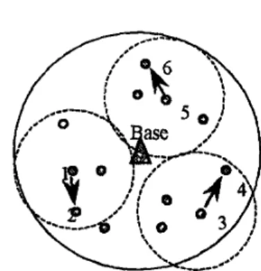
When station i sends a packet to any station in rhe cell, the hop count, mC, is a function of the positions of station i and the destined station. The mean hop count from station i to station j can be computed by fixing the position of one station, say i, so that the distribution of hc _{can be} derived. When station i is located in the gray area in Fig. 6, the hop count ^U, the base will be n because its transmission range equals R/kp. Hence, the probability of station i being located in the nth layer of the cell is n[(

2)2 ^-

( 9 ) 2 ] / 7 r R 2 , which equals (2n

-

l ) / k i , where 1

5

n

5

kp. 'The maximum hop count is known to be kp

+

^{n, n hops to} the base and kp hops from the base to the station located near the boundary of the cell, allowing us to obtain 1

<,

hop wunt 5

le, +

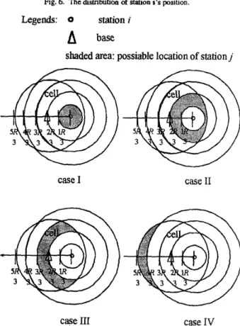
^{n. Fig. 7 shows} four differ- ent cases ^U, compute the probability distribution of hop count, P ( hop count = hc), as derived below under the condition that station i is in the nth layer of the cell:

(caseZ) P ( h o p m n t = h c ) =7r[(hc-R/kp)a- ( ( h c - 1 ) - R / k p ) 2 ] / ~ R 2 , which equals (2hc

-

l)/k;, when 1 hc

5

IC, - n ;

(case ZZ) P ( hop count = h) = (A( hc, n, kp

,

R)

-

ⁿ

-

( (hc

-

1) A / k p ) 2 ) / ~ A 2 , when hc _{= kp}

-

ⁿ

+

1;

(case 111) P(h0p count = hc) = (A(hc,n, k p , R )

-

^{A ( h}

-

1, n, kp, R))/nR2, when k,

-

ⁿ

+

²

⁵

^{hc 5 kp}

+

ⁿ

-

^1; and ( c a s e w ) P(h0p count = hc) = 1

-

^A(hc

-

1, n, kp, R)/7rR2, when hc = kp

+

^n,

where ACj, n, IC,, R) denotes the mean intersection area of two circles with radiuses of R and jR/k,, i.e. the shaded area shown in Fig. 8. Since station i is in the nth layer of the cell, we have (n

-

¹⁾

-

^{R / k p < a}

⁵

ⁿ

-

R / k p . Thus, we can write AG, n, kp, R ) =

~ & t $ ~ , ~ ~

[ol(j~/k~)~+e~2-CG~sinelda,

---

,---

--

Fig. 6. The distribution of station i's position.

Legends: ⁰ stationi

A

base

shaded m a : possiable location of station j

case I case I1

case 111 case IV

Fig. 7. Four cases to compute P(hop count = hc), for k p = 3 and n = 2.

Fig. 8. Definition of A ( j , n, k,, R).

0-7803-5880-5/00/$10.00 ( C) 2000 IEEE 1277 IEEE INFOCOM 2000

where sine = ( j / k , ) - sina, and cos0 = (Ra

+

^u2

-

( j R / ? ~ , ) ~ ) / 2 a R since

R2 -

(Rcos8)a = (iR/A#

-

(a

-

Rcos6)'.

We now get the probability of station i being located in the nth layer is (2n

-

^{l)/kg and the mean} hop count when station i sends a packet to any station in the same cell is ^~~~~ hc

-

P(hop c"!= hc). Thus, the mean hop count, which is a function of kp, can be written as

uvg-hc-ij(kp) =

Fy,

S+n ^{hc * P(hW a n t} = hc). (2)

n=l hc=1

The mean hop count from station i to the base, awg&io(k,), can be computed in a similar manner. How- ever, it is much simpler to obtain a w g h c i o ( b ) because the destination, i.e. the base, is at the fixed position. Thus, uwg-hCio(k,) is given by CF=l((2n

-

^{l)/k;) n, which}

euuals -1-

When the base sends a packet to any station in the cell, a v g h s i ( k p ) obviously equals awghcio(kJ.

System thmughput analysis:

For simplicity, assume that (a) the traffic is uniformly dis- tributed within the cell, (b) stations can always find the next hop to forward packet,, and (c) the base does not help forward packets if the.pair of source and destination is both in the same cell. To analyze the throughput, five major steps are required

1. Derive Xi, G., and Gb. of MCN;

2. Derive t i d l e to obtain the renewal interval;

3. Derive the probability of successful transmission at station i and the base;

4. Derive the hop-by-hop throughput of station i and the base;

and

5. Derive the hop-by-hop throughput and end-to-end through- put of MCN.

By assuming that stations help forward packets, the total rrafiic rate at station i is given as

Xi = Xi0 ^* uVgh-iO(kp)

+

^{X o j *} (avghcio(kp)

-

¹⁾

+

N Aij * a ~ g h - i j ( k p ) , (4)

j#i,j=1

because each packet is, on average, forwarded either awghCij(k,) times if the destination is in the same cell, u w g h i o ( k p ) times if the destination is outside the cell, or a u g h c d ( k p )

-

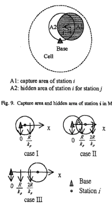
1 times when the source is outside the cell and the first transmission is done by the base. Notably, Xi is intuitively equivalent to the traffic rate handled, i.e. pumped or forwarded, by station i because the traffic rate, to the cell, con- tributed by station i should equal the traffic rate, contributed by others, station i should take care of. Now we denote the traffic

A l : capture area of station i

A2: hidden area of station i for station j Fig. 9. Capture m a and hidden area of station i in MCN.

X R Z R

O R o - -

kF kD kF

case I case

II

n

A

Base

n R 2R

U - -

kD kg 0 Stationi

case

ITI

Fig. 10. "e cases to compute P s i .

rate at all stations and the base by G, and Gbs, which equal

Czl

^Xi and Xoi, respectively.

In MCN, t-idle is derived as l/((G,

+

Gb.)/ki) which equals k i / ( G .

+

Gb,), where the area of a sub-cell is l / k g of the area of a cell. The mean length of a renewal intend is thus defined as

m a d e =

J D I F S

+ +

JRTS

+

r

+

J S I F S

+

ZCTS

+

r +Ps

*

^(ISIFS

+

^{~ P K T}

+

^r

+

IFS

+

^{~ A C K}

+

r ) . ( 5 ) For convenience, we again denote n-h and h as AI JnR2 and A2/n R2, where A1 and A2 are the mean capture area and the mean hidden area, respectively, of station i when it sends a packet to the next hop, say j , as shown in Fig. 9. Now the probability of successful transmission at station i can be de- rived similarIy a.. done in SCN. However, the relative positions of station i and the base have three cases to be considered as shown in Fig. 1 0

(case I )

N

ka

Psi1 = exp { - [ r ( n h

.

^G,

+

^Gb,)

+(2r

+

^{~ R T S}

+

~ I P S ) * h ^* G81), when the distance between station C and the base is smaller than R / k p so that the base is in the capture area of station i;

0-7803-5880-5/00/$10.00 (c) 2000 IEEE 1278 IEEE INFOCOM 2000

A 1 : capture area of the base

A2: hidden ^area of the base for station ⁱ

and Gbe/X[oca[-bs, respectively. We thus derive the hop-by- hop throughput of station i and the base a,,

1 -Psi

xi si=-.---

rn-qde XlOccr(i

’

and

1 ‘Psbs Gbs

s

^--.I__

m - w J e A o c a 1 ~ 8 ’ ba -

respectively. Eventually, the hop-by-hop throughput of MCN is obtained as

sh

=

si +

^{sbs. (6)}

iEcell Fig. 11. Capture m a and hidden area of the base in MCN.

The end-b-end throughput can be written as

when the distance between station i and the base station is larger than R/k, but smaiIer than 2R/k, so that the base would be in the hidden area of station i, with probability PA, when the receiver is positioned in the area A as shown in case II of Fig. 10; and

(case IZI)

Psis = e x p ( - [ r . n h - G ,

+ ( 2 ~

+

^{~ T-t S}I S I F S )

-

^{h. G81Iy}

N N

in which A, B and

C

are Xoi and

cEl

Xio, respectively. This is because each packet from sta- tion i to station j in the same cell is, on average, transmitted avghcij(k,) times and each packet from the b s e to station i or from station i to the base will be transmitted avghcio(lc,) times in MCN. However, only A i j and A~ are going toward

cj=l,j+

^{A i j ,}

those end destinations in the samecell.

be obtained by substituting k, by 1 and R by kb R because, in MCN-b, the transmission range remains the same a, the one in However, the distance bemeen bases is multiplied by when the distance between station and the base is laer than

For the end-m-end throughput of MCN-b, the equations can 2R/k, so that the base does not affect the transmission of sta-

tion i.

From above discussion, we can obtain that the mean proba- bility of successful transmission at station i is

kb ^*

Notably, the hidden area, i.e. A2 in Fig. 11, within the cell should be considered to analyze the probability of successful transmission of the base. We thus write

P8b.g =

exp { - [ r n h

- ^G, +

^(2r

+ ^lms +

^ZSZFS) h

G,]}.

Before deriving the throughput of MCN, we define the lo- cal traflic rate as the mean traffic rate within a sub-cell. Thus, the local trai3c rates at station i and the base are hOcrrli = Notably, the term Gba in X ~ ~ ~ ~ l i is multiplied by l / k i because the probability that the base is in the sub-cell of station i is 1/$. Hence, the probability that a transmission after a re- newal point is fired by either station i or the base is X i / X l o c a l i

(Gs +

^Gbs)/ki and h o c o l ~ s = (Ga/ki)

+

Gb,, respectively.

IV. NUMERICAL RESULTS

Analysis and simulation results for system throughput of SCN and MCN are presented as follows. For simulation re- sults, the SCN and MCN environments are simulated by PAR- SEC [19], a C based discrete-event simulation language de- veloped at UCLA. The values of ^T, ~ P K T , IACX, ~ R T S , ICTS are obtained by using the following parameter values: the data rate is 1.5Mbps, propagation velocity of signals is 3* 1O8m/s, and the length of data, acknowledgment, RTS and C T S pack- ets are 1024, 14,20 and 14 bytes, respectively. However, the value of propagation delay, ^{T ,} is much smaller than the others and, therefore, is neglected in simulations. The other parame- ter values are as follows: the radius of a cell, R, is 150 meters, the number of mobile stations, N, is 250, IDIFS = 0.149 ms, and l s ~ ~ s = 0.042 ms. The total traffic rate in a cell is 167 packets per second, which is about 1.SMbps while consider- ing DIFS, SIFS, RTS and CTS packets, and we normalize this traffic rate, G, to 1, which is the default value.

0-7803-5880-5/00/$10.00 (c) 2000 IEEE 12 79 IEEE INFOCOM 2000

hoD count number of packets / renewal cycle

ZJ' 8 avghop (analysis) ^/' ./

20 ^fi'

15

/

10 8 6 4

2 0

8 avahc-ij (analysis) -A+ avg_hc-ij (simulation)

I I I I

I

1 2 3 4 5 6

kP

Fig. 12. Mean hop count for internal and external traffic in MCN.

Traffic locality,

ELl C&j=l

.Xjj/

ELl

Xi, is defined to compare the end-to-end throughput of SCN and MCN, indi- cating that the percentage of packets generated by any station i, where 1

5

i

5

N, is destined for stations in the same cell.

According to the values of the above parameters. we choose locality = 0.5, and the default value of Zomlity is 0.5. In sim- ulations, the routing table is pre-computed using the all-pairs shortest path algorithm, Floyd-Warshall algorithm [20].

X i j = 0.0008955, Xi, = 0.223 and Xoi = 0.223 SO that

A. Mean hop count vs mean number of channels in MCN Two important factors, mean hop count and mean number of channels, are presented first. which significantly affect the throughput of MCN. Fig. 12 shows the results of mean hop count for internal traffic, i.e. awg,ghc-ij(kp). and for exter- nal traffic, i.e. aughcio(&), in MCN. The curve for ex- temal traffic is lower than the curve for intemal traffic be- cause the maximum hop count from station i to the base is

R/(R/k,)

= kp and the maximum hop count from station i to station j is 2 R / ( R / k p ) = 2kp. For both cases, the hop count increases almost linearly as the transmission range &creases.

When kp _{= 1,} the value of avghc-io(k,) equals 1 because each station i can reach the base in a single hop. However, the value of avghc-ij(kp) is in the interval between 1 and 2 be- cause the hop count may be either l or 2 when station ⁱ wants to send a packet to station j in the same cell. Simulation re- sults show higher values than those of analysis results owing to the assumption when analyzing mean hop count, i.e. station 5 can always find the next hop, at a distance of

R/k,,

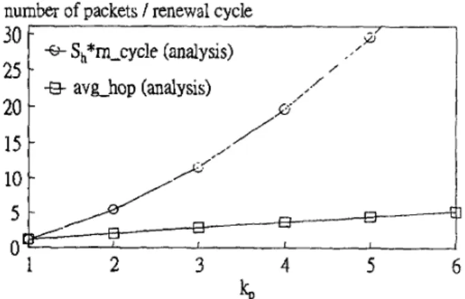
in the straight-line direction towards the destination. The simulation model removes this assumption to reflect the real situation and examine its influence.

Fig. 13 shows the mean number of channels, S b

-

^m_cycle.

i.e. the mean number of packets that can be simultaneously transmitted per renewal cycle within a cell of MCN, and the mean hop count of a packet which is computed as (locality) . avghc-ij(k,)

+

^{( 1}

-

Zocality) -avghc-io(kp). Fig. 14 shows the number of simultaneously received packets at destinations

1

" 1 2 3 4 5 6

k,

Fig. 13. Mean number of channels vs mean hop count.

number of packets I renewal cycle

10

r---

I

-8 S,*m-cycle/avg_hop (analysis)

*

S,*m-cycle (analysis)

k

Fig. 14. End-Wend throughput vs _ratio of mean number of cbannels to mean hop count.

per renewal cycle, i.e. Se

-

r n q c l e , and the ratio of mean number of channels to mean hop count. The former curve is lower than the latter one because of the lack of the term, C.

in numerator in equation (7). As kp increases, Fig. 13 reveals that the number of channels increases much more rapidly at the order close to k: than the mean hop count, which increases at the order close to kp. This result can be explained by closely examining equations (2). (3). (5). and (6). The order of mean hop count, i.e. [ ( l d i t y )

-

⁽⁽²ⁿ

-

^{l)/kg) .}

Ckz:

^hc . from equations (2) and (3). is close to kp. However, the order ofmeannumberof channels, i.e. (5).(6) = k,-[Psi.G8/(G8+

Gas) i- P8bs ^* Gb8/(G,

+

^k~Gas)] from equations (5) and (6), is close to k; because G, is usually much larger than Gbs.

B. SCNvsMCN

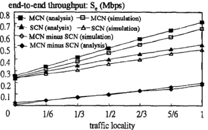
Of particular interest is the difference of the throughput be- tween SCN and MCN. In SCN, each packet is transmitted ex- actly twice. one for upstream and another for downstream, if the destination is in the same cell. However, such a packet is transmitted either once or twice in MCN when kp = 1. When traffic locality is 0, i.e. all packets are sent to the base, the P(hpp m n t = hc)] +[ (1 -lo~ality)*( ( k p + l ) (4kp

-

^1)/6kp)]

0-7803-5880-5/00/$10.00 (c) 2000 IEEE 12 80 IEEE INFOCOM 2000

end-to-end throughput: Se (Mbps)

0 116 113 112 213 516 1

traffic locality

Fig. 15. Impact of traffic locality on throughput fork, = 1 and G = 1.

mean hop count in MCN and SCN are both exactly 1, i.e. no difference between MCN and SCN. However, if traffic local- ity is 1. i.e. the destination is within the cell, the mean hop count in MCN is smaller than the one in SCN as shown in Fig. 12. Hence, the end-to-end throughput is higher m MCN than in SCN. Thus, we predict that a higher locality would in- crease the difference between MCN and SCN. Both "MCN mi- nus S C N curves of analysis and simulation results in Fig. 15 confirm our prediction. For the lack of the term, C, in numer- ator in equation (7), higher locality will increase throughput of both MCN and SCN. However, the end-to-end throughput of simulation results are lower than those of analysis results is caused by the higher value of mean hop count, as shown in Fig. 15.

The curves in Fig. 16 are ascending because the mean num- ber of channels increases much more rapidly than the mean hop count. Figs. 15 and 16 confirm that MCN has a superior throughput than that of SCN. Analysis results in Fig. 16 indi- cate that the upper bound of end-to-end throughput of MCN is reached when G is over 100.

C. MCN-p VS MCN-b

After comparing S C N and MCN, MCNp and MCN-b are compared as follows. In Fig. 17, the dashed circles denote sub-cells, i.e. the transmission ranges of bases, and the solid circles denote celk. Notably, the base of a cell is the closest base for any stations within the cell. Assume that the following two conditions hold

1. kp = kb and the number of stations are the same, i.e. N.

and uniformly distributed within the solid circles of MCNp and MCN-b, respectively.

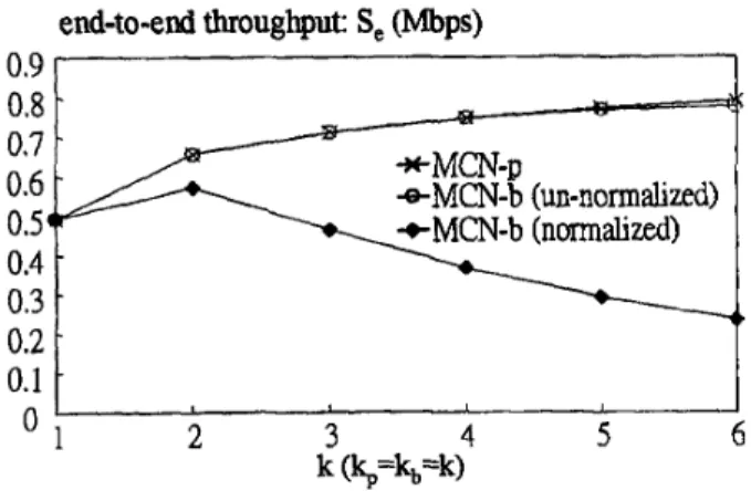
2. The values of Xij, Xi,, and A,; are the same in both MCNp We believe that the end-to-end throughputs of MCN-p and MCN-b are the same, except for the slight difference due to the different propagation delays. In Fig. 18, the two coin- cided curves, "MCN-p" and "MCN-b (un-normalizedY, con- firm above statement. However, the parameters used in MCN- and MCN-b.

0-7803-5880-5/00/$10.00 (c) 2000 IEEE

7 ' 6 ' 5 '

I

O i 2 3 4 5 6

kp

Fig. 16. End-bend throughput under various offered loads in MCN.

MCN-b MCN-I,

Fig. 17. M C N p and MCN-b for 3 = Icb = 2.

b should be normalized to compare the throughput of MCNp andMCN-b, i.e. under the same station density and traffic load within a unit area. Consequently, to compute the throughput of normalizedMCN-b, N is multiplied by ki, and the final result of throughput should also be divided by kf

.

The probability of successful transmission rapidly decreases in MCN-b because the transmission range is kp times of that in MCN-p, i.e. the number of stations in a sub-cell is k% times of that in MCN-p. Above observations account for why the curve of WCN-b (normalized)" in Fig. 18 descends so quickly, im- plying that, given the densities of bases, i.e. R, stations, i.e. N.

and traffic, i.e. A, our formulas help determine the transmission range for the desired throughput level.

V. CONCLUSION

This work presents a new architecture, Multihop Cellular Network (MCN). and derives the throughput of MCN and its counterpart. Single-hop Cellular Network (SCN), ^based on the RTSICTS access method. The throughput is analyzed by mod-

1281 IEEE INFOCOM 2000

end-to-end throughput: Se (Mbps)

0.9

r ¹

0.8 .

+---dc

+MCN-b (un-normalized) 0.4

0.3 0.2 - - -

0.8

1 4

+MCN-b (un-normalized)

0.5 +MCN-b (normalized)

0.1

1

I

2 3 4 5 6

k (k,,=k,,=k)

o i

Fig. 18. 'Ibe difference between MCN-p and MCN-b.

eling the packet departure process as a renewal process, in which the renewal point is defined as the time point when all stations in a sub-cell simultaneously sense that the channel is idle. Furthermore, mean hop count is analyzed because it sig- nificantly influences the throughput of MCN, as confirmed by the numerical results.

Analysis and simulation results for the throughput of SCN and MCN lead to three important observations. First. the throughput of MCN is superior to that of the corresponding SCN. Second, the throughput of MCN increases as the trans- mission range decreases. We explain these two observations by illustrating the different increasing orders, ka and k respec- tively, of mean number of channels, i.e. simultaneous trans- missions in a cell, and mean hop count, as the transmission range decreases by k times. Third, given the densities of bases, i.e. R. stations, i.e. N, and traffic, i.e. A, our formulas help determine the transmission range for the desired throughput level. When the transmission range and distance between bases in MCN-b are kp times of those in MCNp, the number of sta- tions in a sub-cell becomes kg times of that in MCNp and throughput hence descends quickly.

Although MCN shows a higher throughput than SCN, some related issues must be further studied. The first thing is how to obtain an appropriate operational value of k while consid- ering both throughput performance which favors large k and path vulnerability which favors small k. Furthermore, the mo- bility of stations cannot be neglected in the environment with high mobility. Thus, future research should develop an effi- cient routing algorithm and more closely examine the issues of handoff and mobility management in the MCN environment.

ACKNOWLEDGMENT

The authors wish to thank Prof. Tseng-Huei Lee for his in- sightful discussjon on deriving end-to-end throughput.

REFERENCES

[l] Pahlavan and AUen H. Levesque, Wreless lnfonnution Nenvorh, Wiley [2] F. H. Blecher, Advunced mobile phone service, IEEE Trans. Veh. Technol.

[3] T. Hug, OvervioV of GSM: philosophy and res&, Int J. Wireless Inf.

Networks pp.7-16, 1994.

[4] D. Moralee, G"2 ^U new generution of c o d e s s Phones, IEE Review, pp.

177-180, May 1989.

[SI H. Ochsner, DECZ-Digitul Eutopeun Confless Telecommunicruions, 39th IEEEVehicular Tech. Conf., San Francisco, pp. 722-728, May 1989.

[61 W. A. McGladdery and R. Clifford, Survey of currenf und emerging wire- less &tu networks, 1993 Canadian Conference on Electrical and Com- puter Engineering, pp. 1000-1003, Vancouver, Sept. 1993.

[7] K C. BudIra, CeWur &$ul pucket &U - & w e d mobile phone stun- d a d network iwdwidth contention, Proceedings of the 34th IEEE Con- ference on Decision and Control, pp.1941-1946, New Orleans, Dec. 1995.

[8] T. Will;inson, T. G. C. Phipps and S. K. Barton, A report on MPERLAN s t u d d s o n , lnkmational Journal of Wireless information Networks, Vol. 2, No. 2, pp.99-120,1995.

[9] EEf3 Standards Board, Purr 11: Wreless LAN me&um uccess con- ml(MAC) undphysioal t5iyer(PHY) specificutions, The Institute of E l m tical and Electronics Engineers, Inc., IEEE Std 802.11-1997.

[lo] J. Jubin and J. D. Tornow The DARPA pucker d onetwork protocols, Proceedings of IEEE, Vol. 75, No. 1, Jan 1987.

111 B. M. Lemer, D. L. Nielson and F. A. Tobagi, Issues in pucker rudio network design, Proceedings of IEEE, Vol. 75, No. 1, Jan 1987.

121 A. Alwan, R. B a p d i a , N. Bambos, M. Gerla, L. Kleinrock, J. Short, and J. Villasenor, A&pfing to ^U highly vuriabh und unyrem'ctuble envi-

" e n t : uduptive mobile mulrimediu networks, IEEE Personal Commu- nications, pp.3451, April 1996.

131 Y. D. Lin, Y. C. Hsu, K. W. Oyang, T. C. Tsa, and D. S. Yang, Multihop wireless IEEE 802. 11 LAPIS: U prototype implementution, IEEE ICC'99, Vancouver, Canada, June 1999.

Intwscience, pp. 613,1995.

VT-29, pp.238-244,1980.

[14] hup://www.metncom.com/.

[IS] I. E Abyildiz, Wei Yen, and Bulent Yener, A new hierurchicd muring protocol for djnumic multihop wireless networh, IEEE Ih'FOCOM.97,

1997.

[I61 Zygmunt J. Haas, On the per$ormunce of ^U medium uccess control scheme for the reconfiguruble Wireless nemorks, MILCOM'97, pp.1558- 1564,1997

[17] H. S. Chhaya and S. Gupta, Pe?fomumce modeling ofusynchmnous dutu tnm.fer methods of IEEE 802.11 MACptvtocol, Wireless Networks, vol.

[la] F. A. T o w and L. Kleinrock, Pucker switching in rudio chunnels, P u t U: The Wen-tenninul problem in currier sense multiple uccess und the

bus-tonesolution, IEEETrans. Commun., COM-23, pp.1417-1433,1975.

[19] Richard A. Meyer, PARSEC user maw&, http://pcl.cs.ucla.edu/, Aug.

1998.

[a] T. H. Cormen, C. E. Leiserson, and R. L. Rwest, Introduction ro Algo- r i r h m , The MlT F'ress, pp.558-565, 1992.

3, pp.217-234,1997.

0-7803-5880-5/00/$10.00 ( c ) 2000 IEEE 1282 IEEE INFOCOM 2000