606
IEICE TRANS. INF. & SYST., VOL.E90–D, NO.2 FEBRUARY 2007
LETTER
A Low-Complexity Interpolation Method for Deinterlacing
Pei-Yin CHEN†a), Member and Yao-Hsien LAI†, Nonmember
SUMMARY A direction-oriented spatial interpolation technique for image de-interlacing is presented in this letter. The experimental results demonstrate that our method achieves excellent performance in terms of both objective and subjective image quality. The proposed algorithm also has a very computationally simple structure, and proves to be a good can-didate for low-cost hardware interpolator.
key words: interpolation, low-cost 1. Introduction
Various digital video systems need different spatial and tem-poral resolutions, so different format standards are used to store, transmit and display digital video signals. Traditional NTSC-TV uses the interlaced scanning format to display video sequences. It suffers from uncomfortable visual ar-tifacts such as edge flicker, interline flicker and line crawl-ing. Recently, many progressive scanned devices such as HDTV, PDPs and LCD-TVs become more and more popu-lar. Hence, an efficient image de-interlacing (or conversion) technique is necessary to convert the interlaced images into progressive images for suitable displaying.
Interpolation is used widely in image de-interlacing to obtain higher image resolution [1]. In the past few years, many image interpolation methods have been proposed, ranging from spatial techniques [2]–[6] to more complex temporal techniques [7]–[10]. Temporal techniques usually perform better than spatial techniques with regard to image quality, but they require more expensive computations and larger memory space. In contrast, the spatial technique is very suitable for real-time applications due to its simplicity and low computational requirements. In this letter, we con-sider only low-complexity spatial interpolation techniques.
Many spatial interpolation techniques have been pro-posed for image enlargement. In [3], an edge-based line average (ELA) interpolation method was developed. Chen et al. [4] presented an efficient algorithm using two useful measurements defined on the sliding window to increase the accuracy of the ELA algorithm. In [5], Kim et al. employed an adaptive pseudomedian filter to implement an image in-terpolator. Based on the median filter [1] and the modified ELA method [4], a median-based interpolation method is
Manuscript received May 22, 2006. Manuscript revised August 2, 2006.
†The authors are with the Department of Computer Science
and Information Engineering, National Cheng Kung University, Tainan 701, Taiwan, R.O.C.
a) E-mail: pychen@csie.ncku.edu.tw DOI: 10.1093/ietisy/e90–d.2.606
proposed in [6].
In this letter, we present an efficient and low-complexity interpolation method. The proposed method in-troduces additional measurements for estimating the spatial correlations efficiently, with the primary objective of alle-viating decision errors for subsequent interpolation. Com-pared with the previous methods, our method can detect edges efficiently and perform better in terms of both objec-tive and subjecobjec-tive image quality. Furthermore, the method has very low computational complexity, so it can be easily implemented with hardware and applied to many real-time applications.
The rest of this letter is organized as follows. In Sect. 2, the proposed method is described in detail. The simulation results are provided in Sect. 3. Finally, conclusions and re-marks are given in Sect. 4.
2. The Proposed Method
The motivation of the proposed interpolation algorithm is first to estimate efficiently the spatially directional correla-tions, and then to interpolate the missing pixels accordingly. Let x(i, j) denote the signal to be interpolated where i means the number of horizontal line and j means the number of vertical line. The signals x(i− 1, j) and x(i + 1, j) are sup-posed to be available and can be used as the inputs for in-terpolation. For the purpose of checking edges existed in the diagonal, vertical and horizontal directions respectively, four directional differences, denoted as Dd1, Dd2, Dvand Dh, are defined and calculated as follows:
Dd1= |x(i − 1, j − 1) − x(i + 1, j)| + |x(i − 1, j) − x(i + 1, j + 1)| Dd2= |x(i − 1, j) − x(i + 1, j − 1)| + |x(i − 1, j + 1) − x(i + 1, j)| Dv= |x(i − 1, j) − x(i + 1, j)| × 2 Dh= |x(i − 1, j − 1) − x(i − 1, j)| + |x(i + 1, j − 1) − x(i + 1, j)| (1)
Figure 1 shows the four pixel differences of different direc-tions, respectively. The smaller one among these four values has a stronger correlation, and probably has an edge in its direction. Hence, the interpolated pixel can be estimated as follows:
LETTER 607 x(i, j) = x(i, j − 1), if Dh= 0 (x(i− 1, j − 1) + x(i + 1, j) + x(i− 1, j) + x(i + 1, j + 1))/4, if min(Dd1, Dd2, Dv)= Dd1 (x(i− 1, j) + x(i + 1, j − 1) + x(i− 1, j + 1) + x(i + 1, j))/4, if min(Dd1, Dd2, Dv)= Dd2 (x(i− 1, j) + x(i + 1, j))/2, if min(Dd1, Dd2, Dv)= Dv (2)
Obviously, the proposed method requires only simple in-teger operations, such as addition, subtraction and abso-lute value, so it can be easily implemented with hard-ware. The simulation results shown in the following section will demonstrate that our method achieves excellent perfor-mances in both objective and subjective image quality.
(a) Dd1 (b) Dd2
(c) Dv (d) Dh
Fig. 1 Four pixel differences for (a) Dd1, (b) Dd2, (c) Dvand (d) Dh.
(a) (b) (c)
(d) (e) (f)
Fig. 2 Interpolated images of Lena for (a) Original, (b) FOI, (c) ELC, (d) APM, (e) MBI, and (f) Our algorithms.
3. Simulation Results
For an M× N image, we remove every odd vertical line and thus obtain the M/2 × N image. Then, we reconstruct the M× N image by interpolating the odd lines for differ-ent methods. Totally, ten 512× 512 standard test images with 8-bit brightness resolution are considered. The results of peak signal-to-noise ratio (PSNR) are illustrated in Ta-ble 1. Except our method, five previous interpolation meth-ods, FOI [2], ELA [3], ELC [4], APM [5] and MBI [6], are used for comparisons. It can be observed from the results that our algorithm achieves better quantitative quality than the previous interpolation methods. Certainly, the exact de-gree of improvement is dependent on the content of different images being processed.
In addition, three well-known 8-bit gray-level video se-quences, Football, Akiyo and Erik, are used to test various interpolation methods. The size of each frame is 352× 288,
Table 1 Comparison of PSNR for different methods. FOI [2] ELA [3] ELC [4] AMP [5] MBI [6] Ours Baboon 23.42 22.90 23.10 23.46 23.40 23.44 Barbara 30.68 24.78 29.56 29.14 30.42 30.45 Couple 27.96 27.44 27.64 27.88 27.87 27.94 Crowd 31.76 31.19 31.37 31.70 31.68 31.82 F18 23.60 23.18 23.20 23.61 23.59 24.97 Indian 32.05 30.88 31.48 31.85 31.97 32.11 Lake 28.46 27.99 28.09 28.39 28.42 28.47 Lax 26.93 25.91 26.41 26.93 26.91 27.04 Lena 32.28 31.52 32.00 32.29 32.31 32.38 Peppers 29.22 29.33 29.36 29.42 29.36 29.36 AVG 28.64 27.51 28.22 28.47 28.59 28.80
608
IEICE TRANS. INF. & SYST., VOL.E90–D, NO.2 FEBRUARY 2007
Table 2 Comparison of average PSNR for three video sequences. FOI [2] ELA [3] ELC [4] AMP [5] MBI [6] Ours Football 35.99 34.65 34.51 35.68 35.93 36.16 Akiyo 39.94 37.90 39.46 39.55 39.95 40.24 Erik 29.94 29.43 29.71 30.01 29.95 30.06
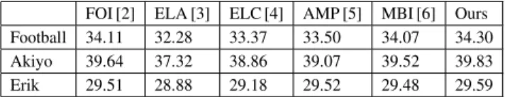
Table 3 Comparison of the worst-case PSNR for three video sequences. FOI [2] ELA [3] ELC [4] AMP [5] MBI [6] Ours Football 34.11 32.28 33.37 33.50 34.07 34.30 Akiyo 39.64 37.32 38.86 39.07 39.52 39.83 Erik 29.51 28.88 29.18 29.52 29.48 29.59
Table 4 Comparison of operations required for different methods. FOI [2] ELA [3] ELC [4] AMP [5] MBI [6] Ours
Absolute 0 3 7 4 5 5
Addition 1 1 3 5 3 5
Subtraction 0 7 13 19 25 11
and the frame rate is 30 per second. Each individual frame is down sample by a factor of 2 vertically, and then inter-polated by using different approaches. Tables 2 and 3 show the average and worst-case PSNR of the first 50 frames for the video sequences respectively. The proposed method consistently produces better performance. This demon-strates the capability of our method in coping with video sequences.
For subjective testing, the interpolated Lena images using different interpolation methods are shown in Fig. 2. A portion of each image is enlarged in order to evaluate the visual quality. FOI produces noticeable artifacts in areas of angled edges as shown Fig. 2 (b). Like those previous pro-posed methods [4]–[6], our method shows visually pleasing picture especially at image edges.
To explore the computational complexity, we list the operations required to interpolate each missing pixel for various interpolation methods in Table 4. Compared with the newly interpolation methods [4]–[6], our method re-quires lower computational complexity (5 absolute, 5 addi-tion and 11 subtracaddi-tion operaaddi-tions). Although the proposed method needs more operations than both FOI and ELA do, it achieves better objective image quality as shown in Tables 1, 2, and 3.
4. Conslusions
A low-complexity spatial interpolation technique is pre-sented to detect edges in the diagonal, horizontal and ver-tical directions efficiently. The experimental results demon-strate that our method achieves excellent performances in both objective and subjective image quality. Currently, the VLSI architecture of our method is under development.
Acknowledgment
This research was supported in part by the National Science Council, Republic of China, under the Grant NSC-95-2221-E-006-504. Also, this work made use of Shared Facilities supported by the Program of Top 100 Universities Advance-ment, Ministry of Education, Taiwan.
References
[1] G.D. Haan and E.B. Bellers, “Deinterlacing–an overview,” Proc. IEEE, vol.86, no.9, pp.1839–1857, Sept. 1998.
[2] R.S. Prodan, “Multidimensional digital signal processing for televi-sion scan convertelevi-sion,” Phillips J. Res., vol.41, pp.576–603, 1986. [3] T. Doyle, “Interlaced to sequential conversion for EDTV
applica-tions,” Proc. 2nd Int. Workshop on Signal Processing of HDTV, pp.412–430, Feb. 1988.
[4] T. Chen, H. Wu, and Z.H. Yu, “Efficient de-interlacing algorithm using edge-based line average interpolation,” Optical Engineering, vol.39, no.8, pp.2101–2105, Aug. 2000.
[5] H.-C. Kim, B.-H. Kwon, and M.-R. Choi, “An image interpolator with image improvement for LCD controller,” IEEE Trans. Consum. Electron., vol.47, no.2, pp.263–271, May 2001.
[6] M.Q. Phu, P.E. Tischer, and H.R. Wu, “A median based inter-polation algorithm for deinterlacing,” Proc. International Sympo-sium on Intelligent Signal Processing and Communication Systems, pp.390–397, 2004.
[7] D. Wang, A. Vincent, and P. Blanchfield, “Hybrid de-interlacing al-gorithm based on motion vector reliability,” IEEE Trans. Circuits Syst. Video Technol., vol.15, no.8, pp.1019–1025, Aug. 2005. [8] X. Gao, J. Gu, and J. Li, “De-interlacing algorithms based on
mo-tion compensamo-tion,” IEEE Trans. Consum. Electron., vol.51, no.2, pp.589–599, May 2005.
[9] S. Yang, Y.Y. Jung, Y.H. Lee, and R.H. Park, “Motion compensa-tion assisted mocompensa-tion adaptive interlaced-to-progressive conversion,” IEEE Trans. Circuits Syst. Video Technol., vol.14, no.9, pp.1138– 1148, Sept. 2004.
[10] O. Kwon, K. Sohn, and C. Lee, “Deinterlacing using directional in-terpolation and motion compensation,” IEEE Trans. Consum. Elec-tron., vol.49, no.1, pp.198–203, Feb. 2003.