國
立
交
通
大
學
資訊科學與工程研究所
碩
士
論
文
引 入 重 組 運 算 子 與 動 態 鏈 結 開 發 技 術 於
粒
子
群
最
佳
法
Introducing Recombination with Dynamic Linkage
Discovery to Particle Swarm Optimization
研 究 生:簡明昌
指導教授:陳穎平 教授
引入重組運算子與動態鏈結開技術於粒子群最佳化演算法
Introducing Recombination with Dynamic Linkage Discovery to
Particle Swarm Optimization
研 究 生:簡明昌 Student:Ming-chung Jian
指導教授:陳穎平 Advisor:Ying-ping Chen
國 立 交 通 大 學
資 訊 科 學 與 工 程 研 究 所
碩 士 論 文
A ThesisSubmitted to Institute of Computer Science and Engineering College of Computer Science
National Chiao Tung University in partial Fulfillment of the Requirements
for the Degree of Master
in
Computer Science
June 2006
Hsinchu, Taiwan, Republic of China
引入重組運算子與動態鏈結開發技術
於粒子群最佳化演算法
學生:簡明昌 指導教授:陳穎平
國立交通大學資訊科學與工程研究所
摘 要
粒子群最佳化演算法(PSO)為一有效率之演化計算演算法,近年更有許多改良粒子群最 佳化演算法的研究持續進行中,其中針對粒子群最佳化演算法與基因演算法(GAs)之結 合的主題亦已成為熱門研究。另一方面,於基因演算法中,如何有效處理基因鏈結 (Genetic linkage)問題亦成為有效改良基因演算法效能的重要議題。因此於本論文中, 主要欲達成之目標有二。第一,我們透過引入基因鏈結之概念於粒子群最佳化演算法 中,藉以提昇其搜尋之效能。為了完成之目標,我們必須瞭解粒子群最佳化演算法及基 因鏈結問題之特性,並尋找適當的結合模式以有效發揮兩者的功能。除此之外,我們希 望能完成之另一目標為有效處理、辨識實數問題之基因鏈結,而為達成此一目標,我們 必須設計一個特別的基因鏈結辨識技術。 於此篇論文中,我們假設基因鏈結於實數問題中是存在且隨著搜尋過程中而產生變動。 於此假設前提下,我們設計了動態基因鏈結開發技術(dynamic linkage discovery technique)來處理基因鏈結問題,此技術為根據適者生存之自然淘汰為概念所設計,為 有效且計算成本低廉的基因鏈結辨識技術。此外,為了有效提昇粒子最佳化演算法及基 因鏈結辨識結合的效能,我們亦設計了重組運算子(recombination operator),透過操 作使用動態基因鏈結開發技術所辨識出的建構基石(building blocks),粒子群最佳化 演算法便能有效的處理存在於實數問題中的基因鏈結,於此研究中,我們將結合重組運 算子、動態鏈結開發技術與粒子群最佳化的演算法稱為PSO-RDL。 因此於此研究中,我們藉由引入動態基因鏈結開發技術來處理實數問題中的基因鏈結, 搭配重組運算子的運作以提昇粒子群最佳化演算法的效能。我們透過仔細設計的各項數學函式做為評估實驗,針對所提出的演算化做效能上的評估分析。另外,我們也將 PSO-RDL應用於電力系統上的經濟調配問題,而由各項實驗的結果也可知,我們所設計 的演算法確有完成提昇效能的目標。
關鍵詞: 粒子群最佳化演算法; 基因演算法; 基因鏈結; 建構基石; 動態基因鏈結開發
iii
Introducing Recombination with Dynamic Linkage
Discovery to Particle Swarm Optimization
Student: Ming-chung Jian Advisor: Ying-ping Chen
Institute of Computer Science and Engineering
College of Computer Science
National Chiao Tung University
Abstract
There are two main objectives in this thesis. The first goal is to improve the performance of the particle swarm optimizer by incorporating linkage concept which is an essential mechanism in genetic algorithms. To achieve this purpose, we need to know the characteristics of the particle swarm optimizer and the genetic linkage problem. Through survey of the particle swarm optimization and the linkage problem, we then figure out how to introduce the linkage concept to particle swarm optimizer. Another goal is to address the linkage problem in real-parameter optimization problems. We have to study different linkage learning techniques, and understand the meaning of genetic linkage in real-parameter problems. After that, we design a novel linkage identification technique to achieve this objective.
iv
that genetic linkages are dynamically changed through the search process are the primary assumptions. With these assumptions, we develop the dynamic linkage discovery technique to address the linkage problem. Moreover, a special recombination operator is designed to promote the cooperation of particle swarm optimizer and linkage identification technique. In the consequence, we introduce the recombination operator with the technique of dynamic linkage discovery to particle swarm optimization (PSO). Dynamic linkage discovery is a costless, effective linkage recognition technique adapting the linkage configuration by utilizing the natural selection without incorporating extra judging criteria irrelevant to the objective function. Furthermore, we employ a specific recombination operator to work with the building blocks identified by dynamic linkage discovery. The whole framework forms a new efficient search algorithm and is called PSO-RDL in this study. Numerical experiments are conducted on a set of carefully designed benchmark functions and demonstrate good performance achieved by the proposed methodology. Moreover, we also applied the proposed algorithm on the economic dispatch problem which is an essential topic in power control systems. The experimental results show that PSO-RDL can performs well both on numerical benchmark and real-world applications.
keywords:
Particle swarm optimization, genetic algorithms, genetic linkage, building blocks, dynamic linkage discovery, recombination operator
v
誌謝
本論文得以順利完成,首先特別要感謝我的指導教授陳穎平老師的
細心指導與諄諄教誨,感謝老師於兩年來細心與耐心的指導以及對我孜
孜不倦的教誨,使我不僅在研究過程中受益良多,且在待人處世各方面
均有許多的成長,謹致上最誠摯的謝意。
口試期間,承蒙孫春在老師、鍾雲恭老師,洪炯宗老師提供許多寶
貴的意見並逐字斧正,使本論文呈現更完整的面貌,他們對學生的提攜
以及謙沖的風範,將永記在心。
感謝於論文撰寫期間,自然計算實驗室的成員劉柏甫、謝長泰、洪
秉竹、陳宏偉、林盈吟、李文瑜等各位學長、同學及學弟妹的協助,讓
我在遇到困難及心情低落時能獲得適時的支持與鼓勵,有了你們的陪伴
讓我兩年的研究生活顯得多采多姿且值得回憶。
最後,感謝我一生中最重要的家人在此期間的體諒、支持與鼓勵,
讓我可以無後顧之憂的專心於學業上,你們是我在論文寫作過程中最重
要的精神後盾,謹將此論文獻給你們,謝謝你們。
簡明昌 謹誌
中華民國九十五年六月
Contents
Abstract i
Table of Contents vi List of Figures viii
List of Tables ix
1 Introduction 1
1.1 Motivation . . . 1
1.2 Thesis Objectives . . . 2
1.3 Road Map . . . 3
2 Particle Swarm Optimization 5 2.1 Historical Background . . . 5
2.2 Particle Swarm Optimization . . . 6
2.3 Parameters of PSO . . . 8
2.4 Recent Advances in PSO . . . 9
2.5 Summary . . . 10
3 Genetic Linkage 12 3.1 What Is Genetic Linkage? . . . 12
3.2 Why Is Genetic Linkage Important? . . . 14
3.3 Genetic Linkage Learning Techniques . . . 15
4 Framework 17
4.1 Dynamic Linkage Discovery Technique . . . 17
4.2 Recombination Operator . . . 20
4.3 Introducing Recombination with Dynamic Linkage Discovery in PSO . . . 22
4.4 Summary . . . 23 5 Experimental Results 26 5.1 Test Functions . . . 26 5.2 Parameter Setting . . . 29 5.3 Experimental Results . . . 29 5.4 Discussion . . . 30 5.5 Summary . . . 43 6 Real-world Applications 46 6.1 Economic Dispatch Problem . . . 46
6.2 Our Solution . . . 48 6.3 Experiments . . . 49 6.3.1 Test Problems . . . 49 6.3.2 Experimental Results . . . 50 7 Conclusions 56 7.1 Summary . . . 56 7.2 Future Work . . . 57 7.3 Main Conclusions . . . 58 A CEC’05 25 Real-Parameter Functions 60 B Global Optimum for CEC’05 25 Real-Parameter Functions 71 C Solutions found by PSO-RDL for CEC’05 25 Real-Parameter Functions 73
List of Figures
2.1 Flowchart of Particle Swarm Optimizer . . . 11 4.1 flowchart of the dynamic linkage discovery process . . . 19 4.2 An illustration of linkage identification . . . 20 4.3 The procedure of how a new particle is generated through the
recombina-tion operator . . . 21 4.4 The process of constructing new population through recombination operator 22 4.5 Pseudocode of PSO-RDL . . . 24 4.6 The flow of the PSO-RDL . . . 25 5.1 Fitness convergence and linkage dynamics of the Sphere function . . . 41 5.2 Fitness convergence and linkage dynamics of the Shifted Rotated Griewank’s
function . . . 44 5.3 Fitness convergence and linkage dynamics of the Shifted Expanded Griewank’s
plus Rosenbrock’s function. . . 44 5.4 Fitness convergence and linkage dynamics of the Shifted Rastrigin’s function. 45
List of Tables
5.1 Related parameters of test functions . . . 28
5.2 Parameter setting in this numerical experiments . . . 29
5.3 Experimental results for test functions 1-5 . . . 31
5.4 Experimental results for test functions 6-10 . . . 32
5.5 Experimental results for test functions 11-15 . . . 33
5.6 Experimental results for test functions 16-20 . . . 34
5.7 Experimental results for test functions 21-25 . . . 35
5.8 Comparison with other algorithms for functions 1-5 . . . 36
5.9 Comparison with other algorithms for functions 6-10 . . . 37
5.10 Comparison with other algorithms for functions 11-15 . . . 38
5.11 Comparison with other algorithms for functions 16-20 . . . 39
5.12 Comparison with other algorithms for functions 21-25 . . . 40
5.13 Problems solved in different evolutionary algorithms . . . 41
6.1 Parameters to 3-unit system . . . 50
6.2 Parameters to 40-unit system . . . 52
6.3 Result for 3-unit system . . . 53
6.4 Result for 40-unit system . . . 53
6.5 Generation output for 40-unit system . . . 54
6.6 100 trial result for 40-unit system . . . 55
6.7 t-Test results for PSO-RDL and MPSO I . . . 55
6.8 t-Test results for PSO-RDL and MPSO II . . . 55
Chapter 1
Introduction
1.1
Motivation
Particle swarm optimizer (PSO), introduced by Kennedy and Eberhart in 1995 [1, 2], emulates flocking behavior of birds to solve optimization problems. The PSO algorithm is conceptually simple and can be implemented in a few lines of codes. In PSO, each potential solution is considered as a particle. All particles have their own fitness values and velocities. These particles fly through the D-dimensional problem space by learning from the historical information of all the particles. There are global and local versions of PSO. Instead of learning from the personal best and the best position discovered so far by the whole population as in the global version of PSO, in the local version, each particle’s velocity is adjusted according to its own best fitness value and the best position found by other particles within its neighborhood. Focusing on improving the local version of PSO, different neighborhood structures are proposed and discussed in the literature. Moreover, the position and velocity update rules have been modified to enhance the PSO’s performance as well.
On the other hand, genetic algorithms (GAs), introduced by John Holland [3, 4], are stochastic, population-based search and optimization algorithms loosely modeled after the paradigms of evolution. Genetic algorithms guide the search through the solution space by using natural selection and genetic operators, such as crossover, mutation, and the like. Furthermore, the GA optimization mechanism is theorized by researchers [3, 4, 5] with building block processing, such as creating, identifying and exchanging. Building blocks are conceptually non-inferior sub-solutions which are components of the superior
complete solutions. The building block hypothesis states that the final solutions to a given optimization problem can be evolved with a continuous process of creating, identifying, and recombining high-quality building blocks. According to that the GA’s search capa-bility can be greatly improved by identifying building blocks accurately and preventing crossover operation from destroying them [6, 7], linkage identification, the procedure to recognize building blocks, plays an important role in GA optimization.
The two aforementioned optimization techniques are both population-based that have been proven successful in solving a variety of difficult problems. However, both models have strength and weakness. Comparisons between GAs and PSOs can be found in the literature [8, 9] and suggest that a hybrid of these two algorithms may lead to further ad-vances. Hence, a lot of studies on the hybridization of GAs and PSOs have been proposed and examined. Most of these research works try to incorporate genetic operators into PSO [10, 11], while some try to introduce the concept of genetic linkage into PSO [12]. Based on the similar idea employed by linkage PSO[12], our work is to introduce recom-bination working on building blocks to enhance the performance of PSO with the concept of genetic linkage.
1.2
Thesis Objectives
This thesis presents a research project that aims to address the genetic linkage problem in real-parameter optimization problems and introduce the genetic linkage concept to particle swarm optimizer. Thus, there are two primary objectives:
1. With the assumption that linkage problems exist in real-parameter problems , a linkage identification technique is needed to address the genetic linkage problems. This thesis provides both the linkage identification mechanism and observation of experiments to support the initial assumption.
2. To improve the performance of particle swarm optimizer, the genetic linkage concept is introduced. An optimization algorithm that incorporates these mechanism is developed and numerical experiments are done to evaluate the performance.
Focusing on the two objectives, in this research work, we propose a dynamic linkage discovery technique to effectively detect the building blocks of the objective function. This technique differs from those traditional linkage detection technique in that the evaluation cost is eliminated. The idea is to dynamically adapt the linkage configuration according to the search process and the feedback from the environment. Thus, this technique is costless and easy to be integrated into existing search algorithms. Our method introduces the linkage concept and the recombination operator to the operation of particle swarm optimizer.
1.3
Road Map
This thesis is composed by six chapters. The detailed organization is given as follows: • Chapter 1 consists of the motivation, objectives and organization of this study. It
describes why this research work is important and the main tasks to be accom-plished.
• Chapter 2 provides a complete overview of the particle swarm optimization algo-rithm. The background and traditional particle swarm optimizer is introduced, and the parameter controls that have an impact on the performance are discussed. Moreover, recent advances of related work in particle swarm optimization are also surveyed in this chapter.
• Chapter 3 presents the concept of genetic linkage in genetic algorithms. The defin-ition and importance of genetic linkage are described. Linkage learning techniques in the literature are also briefly discussed.
• Chapter 4 described the proposed method in detail. The three mechanisms including particle swarm optimizer, dynamic linkage discovery technique and recombination operator, are introduced. The algorithm composed by the above three components is then presented.
• Chapter 5 shows the numerical experimental results that evaluate the performance of the proposed algorithm. The description of the test functions, parameter settings,
and simulated results are given. The discussion and observation of the experiments are covered in this chapter certainly.
• Chapter 6 applied the designed algorithm on economic dispatch problems, which are a significant topic in the power system. It describes the objectives and formu-lations of economic dispatch problems, and then gives the proposed solution and experimental results.
• Chapter 7 give a summary of this research work. The future works and the main conclusions of the study are proposed.
Chapter 2
Particle Swarm Optimization
The particle swarm optimizer (PSO), introduced by Kennedy and Eberhart in 1995 [1, 2], emulates flocking behavior of birds to solve the optimization problems. The PSO algorithm is conceptually simple and can be implemented in a few lines of codes. In PSO, each potential solution is considered as a particle. All particles have their own fitness values and velocities. These particles fly through the D-dimensional problem space by learning from the historical information of all the particles. In the following sections, we will give a complete overview of PSO. Section 1 introduces the historical background of PSO, section 2 describes how PSO works, section 3 discusses the parameter control in PSO, section 4 has a brief survey of PSO related to our work, and finally, section 5 gives a summary of this chapter.
2.1
Historical Background
Many scientists have studied and created the computer simulation of various interpreta-tions of the movement of organisms in a bird flock or fish school [13, 14]. From simulainterpreta-tions, it is considered that there might be a local process that underlies the group dynamics of bird social behavior and relies heavily on manipulation of inter-individual distance. That is, the movement of the flock was an outcome of the individuals’ efforts to maintain an optimum distance from their neighborhood [1].
The social behavior of animals and in some cases of humans, is governed by similar rules. However, human social behavior is more complex than a flock’s movement for at least one obvious reason: collision. Two individuals can hold identical attitudes and
beliefs without banging together, while two birds cannot occupy the same position in space without colliding. Such an abstraction in human social behavior has comprised a motivation for developing a model for it.
As sociobiologist E.O. Wilson [15] has written, ”In theory at least, individual mem-bers of the school can profit from the discoveries and previous experience of all other members of the school during the search for food. This advantage can become decisive, outweighing the disadvantages of competition for food items, whenever the resource is unpredictably distributed in patches”. This statement and numerous examples coming from nature enforce the view ,that social sharing of information among the individuals of a population may offers an evolutionary advantage. This belief has formed a fundamental of the development of particle swarm optimization, which will be introduced in the next section.
2.2
Particle Swarm Optimization
As mentioned above, PSO began as a simulation of a simplified social behavior that was used to visualize the movement of a birds’ flock. Considering such as nearest-neighbor velocity matching, the cornfield vector and acceleration by distance, several variation of the simulation model has been through a trial and error process and finally results in a first simplified version of PSO [1].
PSO is similar to genetic algorithm in that both of them are population based search algorithms. A population of individuals is randomly initialized where each individual is considered as a potential solution of the problem. Especially an individual is called a ”particle” and a population is called a ”swarm” in PSO [1]. However, in PSO, each potential solution is also assigned an adaptable velocity that enables the particle to fly through the hyperspace. Moreover, each particle has a memory that keeps track of the best position in the search space that it has ever visited [2]. Thus the movement of a particle is an aggregated acceleration towards its best previously visited position and the best individual of its neighborhood.
difference between the two variant is that one with a global neighborhood while the other with a local neighborhood. According to the global variant, particle’s movement is influenced by its previous best position and the best particle of the whole swarm. On the other hand, each particle moves according to its previous best position and the best particle of its restricted neighborhood in the local variant. Because the local version of PSO can be derived from the global variant through minor changes. In the next paragraph, we will have a complete introduction of the global version PSO.
In PSO, each particle is treated as a point in a D-dimensional space. Ths ith particle is represented by a D-dimensional vector, Xi = (xi1, xi2, ..., xiD) The best previous position
of any particle is represented as Pi = (pi1, pi2, ..., piD), and the best particle’s position of
the whole swarm is represented by Pg = (pg1, pg2, ..., pgD). The velocity of particle i is also
represented as a D-dimensional vector,Vi = (vi1, vi2, ..., viD). The position and velocity of
each particle is updated according to the following equation:
vidn+1 = vidn + c1∗ randd1() ∗ (pnid− xnid) + c2∗ randd2() ∗ (pngd− xnid) (2.1)
xn+1id = xnid+ vidn+1 (2.2) where d = 1,2,...,D; i = 1,2,...,N , and N is the size of the swarm; c1 and c2 are two
positive constants, called the acceleration constant; rand1() and rand2() are two uniformly
distributed random numbers in the range [0,1]; and n = 1,2,..., determines the iteration number. The second part of the Equation 2.1 is the ”cognition” part, which represents the private thinking of the particle itself, and the third part is the ”social” part, which represents the collaboration among the particles [16]. A flowchart of how the particle swarm optimization works on a swarm is shown in Figure2.1.
Equation 2.1 and 2.2 define the initial version of the PSO algorithm. Referring to Equation 2.1, the second and third part have an important influence on the movement of each particle. Without these two parts, the particles will keep on flying at the current speed in the same direction until they hit the boundary. On the other hand, without the first part of equation 2.1, the particle’s velocity is determined by the current best position
and previous best position. Thus all the particles will tend to move toward the same position. In such a case, it is more likely that the second and third part of the Equation 2.1 play as a local searcher, while the first part plays as a global searcher. There is a tradeoff between the local and global search. For different problems, different balance between them should be considered. In order to achieve this goal, a parameter the called inertia weight ’w’ is introduced, and the Equation 2.1 is modified as [17]:
vidn+1 = w ∗ vnid+ c1∗ randn1() ∗ (pnid− xnid) + c2∗ randn2() ∗ (pngd− xnid) (2.3)
Since the particle swarm optimization is conceptually simple and can be easily imple-mented, the fine-tune of parameters become an important topic which have great impact on the performance of the particle swarm optimization. Discussion about the parameters will be given in the next section.
2.3
Parameters of PSO
In the previous section, we have introduced PSO algorithm and given a modified version. In order to facilitate the efficiency of PSO algorithm, it is important to understand how the parameters would influence PSO. Thus, in this section, we will have a brief discussion on this topic.
Since the particles are ”flying” through the search space, it is necessary to have a maximum value Vmax on it. The parameter has been proven to be crucial because it
actually serves as a constraint that controls the maximum global exploration ability that PSO can have [18]. Moreover, the inertia weight described in Equation2.2 is also important for the balance of global and local search ability. When Vmaxis large, PSO can have a large
range of exploration by selecting a proper inertia weight. By setting a small maximum velocity, PSO would act as a local searcher whatever the inertia weight is selected. As Shi and Eberhart suggested in [18], since the maximum velocity affects global exploration indirectly, it is considered better to controls the global exploration ability through the inertia weight only. Furthermore, choosing a large inertia weight to facilitate greater
global exploration is not a good strategy, and a smaller inertia weight should be selected to achieve a balance between global and local exploration for a faster search.
The parameters c1 and c2 represent the acceleration rates of cognitive and social parts
of each particle. Thus, fine-tuning could result in faster convergence of the swarm. As default values in [1], c1 = c2 = 2 were proposed. Recent work has suggested that it might
be better to choose a larger cognitive parameter, c1, but c1+ c2 ≤ 4 [19].
Finally, rand1() and rand2() are random numbers uniformly distributed in the range
[0,1] and are used to maintain the diversity of the whole swarm.
In the past decade, many studies of improving the performance of particle swarm opti-mization were done. Variants of particle swarm optiopti-mization are discussed and proposed. In the next section, related works in the literature will be given.
2.4
Recent Advances in PSO
In this section, we will have a brief survey of PSO which is related to our research. As mentioned previously, there are mainly two variants of PSO developed and we have given an overview of the global one. However, many researches on the local version of PSO have been working on. In the local variant, the Pg has been replaced by Pl, the best position
achieved by a particle within its neighborhood. Focusing on improving the local version of PSO, different neighborhood structures have been proposed and discussed [20, 21, 22]. Furthermore, studies on modifying the rule of updating position and velocity are also conducted [12, 23, 24]. Devicharan and Mohan [12] first computed the elements of linkage matrix based on observation of the results of perturbations performed in some randomly generated particles. These elements of the linkage matrix were used in a modified PSO algorithm in which only strongly linked particle positions were simultaneously updated. Liang et al [23, 24] proposed a learning strategy where each dimension of a particle learned from particle’s historical best information, while each particle learned from different par-ticles’ historical best information for different dimensions.
In order to enhance the performance of PSO by introducing the genetic operators and/or mechanisms, many hybrid GA/PSO algorithms have been proposed and tested on
function minimization problems [10, 11, 25, 26] Lvbjerg et al [10] incorporated a breeding operator into the PSO algorithm, where breeding occurred inline with the standard ve-locity and position update rules. Robinson et al [25] tested two hybrid version. The first used the GA algorithm to initialize the PSO population while another used the PSO to initialize the GA population. Shi et al [26] proposed two approaches. The main idea of the proposed algorithm was to parallelly integrate PSO and GA. Settles and Soule [11] combined the standard velocity and position update rules of PSO with the concept of selection, crossover, and mutation from GAs. They employed an additional parameter, the breeding ratio, to determine the proportion of the population which underwent the breeding procedure (selection, crossover, and mutation) in the current generation.
Based on the brief literature review, we know that since PSO was proposed, many research focusing on improving the performance of PSO were conducted. By incorporating different mechanisms such as special neighborhood structure, modified update equation or hybridizing with GA concepts, many different models of PSO were developed. In this research work, we have also proposed a particular model of PSO which dissimilar to those described in this section. A detailed description will be given in Chpater 3.
2.5
Summary
In this chapter, particle swarm optimization algorithms were briefly introduced, including its historical background and working principles. The initial and modified global version PSO were described. In order to understand how parameters affect the PSO, we make a short discussion of the parameter control in PSO. Finally, recent advances of PSO that are related to our research work were surveyed. From the survey, we know that the hybridization of PSO and GAs has became a popular research topic. It inspired us to improve the particle swarm optimizer by incorporating the linkage concept in GAs. A complete review of the genetic linkage in GAs will be provided in the next chapter.
Initialize position X, associated velocities V, pbest and gbest of the population
i = 1
d = 1
( )i ( i)
Fitness X >Fitness pbest
d D<
( )i ( )
Fitness X >Fitness gbest
d = d+1 _ i population size< i = i+1 i i pbest = X i gbest X= Yes No Yes Yes Yes No 1* 1 ()*( ) 2* 2 ()*( ) d d d d d d d d i i i i i i i d d d i i i
V V c rand pbest X c rand gbest X
X X V
= + − + −
= +
Figure 2.1: A flowchart of particle swarm optimizer, in each generation, PSO manipulate each particle through updating their position and velocity according to Equation 2.1 and Equation 2.2. After updating particle’s position and velocity, PSO then evaluates particle’s fitness value and decides that the previous best individual and the global best individual should be replaced or not
Chapter 3
Genetic Linkage
In this chapter, we discuss about the topic of genetic linkage in genetic algorithms. We will present the definition and the importance of genetic linkage. The genetic linkage learning techniques are also discussed. Particularly, the following topics are presented:
• The definition of genetic linkage: Describes what genetic linkage is in genetic algo-rithms.
• The importance of genetic linkage: Describes why linkage learning is an essential topic in genetic algorithms.
• The linkage learning techniques: Describes what kinds of techniques have been developed to address the genetic linkage problems.
3.1
What Is Genetic Linkage?
Since the central topics in this chapter is genetic linkage, we first give the definition of genetic linkage in genetic algorithms. The basic idea and assumption of genetic algorithms will be given, and then the definition of genetic linkage in genetic algorithms will be explained.
Genetic algorithms (GAs), introduced by John Holland [3, 4], are stochastic, population-based search and optimization algorithms loosely modeled after the paradigms of evolu-tion. Genetic algorithms search the solution space by using natural selection and genetic operators, such as crossover, mutation, and the like. Furthermore, the GA optimiza-tion mechanism is theorized by researchers [3, 4] with building block processing, such as
creating, identifying and exchanging. Building blocks are conceptually non-inferior sub-solutions which are components of the superior complete sub-solutions. The building block hypothesis states that the final solutions to a given optimization problem can be evolved with a continuous process of creating, identifying, and recombining high-quality building blocks.
For genetic algorithms, the chromosome is represented as a string of characters, and we use genetic operators like crossover and mutation to manipulate these chromosomes. Holland indicated that crossover operator in genetic algorithms induce a linkage phenom-enon [3]. In [27], the term genetic linkage has been loosely defined for a set of genes as follows:
If the genetic linkage between these genes is tight, the crossover operator disrupts them with a low probability and transfers them all together to the child individual with a high probability. On the other hand, if the genetic linkage between these genes is loose, the crossover operator disrupts them with a high probability and transfers them all together to the child individual with a low probability.
This definition implies the genetic linkage of a set of genes depend on the chromosome representation and the crossover operator.
From the definition of genetic linkage given above, we can infer that the linkage phe-nomenon is induced by using crossover operator with string type representation. For example, consider a 6-bit function consisting of two independent subfunctions. For x = [x1, x2, x3, x4, x5, x6], two possible combinations of subfunctions are shown as
fol-lows:
F1(x) = f1(x1, x2, x3) + f2(x4, x5, x6)
F2(x) = f1(x1, x3, x5) + f2(x2, x4, x6)
Taking one-point crossover as an example, it is obviously to see that genes belonging to the same subfunction are likely to stay or to be transferred together in F1(x), while
in F2(x), genes belonging to the same subfunction are split almost every time when a
In Goldberg’s design decomposition [5], the first step to design a competent genetic algorithm is to know what genetic algorithms process. It emphasizes that genetic algo-rithms work through the components of good solutions - identified as building blocks by Holland [3]. Therefore, from the viewpoint of genetic algorithms, genetic linkage can be used to describe and measure the relation of genes, i.e, how close those genes belonging to a building block are on a chromosome.
With the definition of genetic linkage, we can understand that handling genetic linkage is important to genetic algorithms. Hence, we will discussed the influence of the genetic linkage to genetic algorithms in the next section.
3.2
Why Is Genetic Linkage Important?
In the previous section, we give the explanation of what genetic linkage is and the linkage problem occurs when the crossover operator is used. In this section, we will discussed the importance of genetic linkage and how it affects the performance of genetic algorithms.
In many problems, because of the interactions between parameters, to optimize each dimension of candidate solutions separately could not lead to a global optimum. As described in the previous section, linkage, i.e, interrelationships existing between genes needed to be considered when genetic algorithms are used. Moreover, according to Gold-berg’s design decomposition theory, building block identification or genetic linkage learn-ing is critical to the success of genetic algorithms.
Goldberg, Korb, and Deb [6] have used an experiment to demonstrate how genetic linkage dictate the success of a simple genetic algorithm. In the experiment, the ob-jective function is composed of 10 uniformly scaled copies of an order-3 fully deceptive function [28, 29] Three types of codings scheme were tested: tightly ordering, loosely ordering, and randomly ordering. For tightly ordering, genes of the same subfunction are arranged to one another on the chromosome. The loosely ordering coding scheme means that all genes are distributed evenly so that genes belonging to the same subfunction are divided by other genes. The randomly ordering indicates that genes are arranged randomly in an arbitrary order. From the experimental results, it is shown that genetic
algorithms perform well when tightly ordering coding scheme, i,e. genes belonging to the same building block are tightly linked, is used. Moreover, some other studies [30, 31, 4] have also reached similar conclusions. With tight building blocks on the chromosome, genetic algorithms could work better.
From the related work described above, it is clear that one of the essential keys for ge-netic algorithms to success is to handle gege-netic linkage well. The gege-netic linkage problem including all kinds of building block processing such as creation, identification and recom-bination. However, in the real world problem, information about the genetic linkage can not often be known in advance. Thus, studies on handling genetic linkage are extremely important and have long been discussed and recognized in the field of genetic algorithms.
3.3
Genetic Linkage Learning Techniques
The definition and importance of genetic linkage are described in the previous sections. One of the key elements to success in genetic algorithms is to address the linkage prob-lem. In Goldberg’s design decomposition, genetic algorithms capable of learning genetic linkages and identifying good building blocks can solve problems quickly, accurately and reliably. Thus, many research efforts have been concentrated on linkage identification of genetic algorithms, which can be broadly classified into three categories[5]:
• Perturbation techniques include the messy GA [6], fast messy GA [32], gene expres-sion messy GA [33], linkage identification by nonlinearity check GA, and linkage identification by monotonicity detection GA [34], and dependency structure matrix driven genetic algorithms(DSMDGA) [35]
• Linkage adaptation techniques [36, 37]
• Probabilistic model building techniques include population-based incremental learn-ing [38], the bivariate marginal distribution algorithm [39], the extended compact GA (eCGA) [40], iterated distribution estimation algorithm [41], Bayesian opti-mization algorithm(BOA) [42, 43].
For perturbation techniques, the relations between genes are detected by perturbing the value of gene, and analyze the differences before and after the perturbation. For example, linkage identification by nonlinearity check for real-coded GAs (LINC-R) [34] tests nonlinearity by random perturbations on each locus and identifies the linkage con-figuration according to the nonlinearity relation between locus.
In the linkage adaptation technique, linkage learning GA(LLGA) [36, 37] applies a two-point-like crossover operator to ring-shaped chromosomes and constructs linkages dynamically.
According to the probabilistic model building technique, a probabilistic model is built through analyzing the properties and statistics of the population. As an exam-ple, Bayesian optimization algorithm (BOA) [42, 43] constructs a Bayesian network based on the distribution of individuals in a population and identifies linkages.
3.4
Summary
In this chapter, we focus on an important issue in genetic algorithms—genetic linkage. By providing the definition and discussing the importance of the genetic linkage, it is obvious that addressing genetic linkage problem plays an important role for using genetic algorithms. Thus many genetic linkage identification techniques were proposed in the literature. Here we broadly classified them into three categories and had brief explanations for them. The influences of genetic linkage to genetic algorithms inspired us to introduce such a concept to the particle swarm optimizer. Particularly we design a special linkage identification technique which is quite different from those mentioned in this chapter. The proposed framework will be discussed in detail in the next chapter.
Chapter 4
Framework
In this chapter, we will give the overview of the algorithm proposed in this study. This algorithm introduces the recombination operator with the technique of dynamic linkage discovery to particle swarm optimization (PSO) in order to improve the performance of PSO. Dynamic linkage discovery is a costless, effective linkage recognition technique adapting the linkage configuration by utilizing the natural selection without incorporating extra judging criteria irrelevant to the objective function. Furthermore, we employ a specific recombination operator to work with the building blocks identified by dynamic linkage discovery. The following topic will be discussed in this chapter:
• Dynamic linkage discovery technique: Describe how the linkage problem is addressed through the natural selection and dynamic linkage discovery.
• Recombination operator: In order to make good use of building blocks , a special recombination operator which is similar to multi-parental crossover operators is designed and presented here.
• Introducing recombination with dynamic linkage discovery in PSO: A new optimiza-tion algorithm which is composed by particle swarm optimizer, dynamic linkage discovery and recombination operator is described in detail.
4.1
Dynamic Linkage Discovery Technique
From chapter 3, the importance of genetic linkage has been discussed. Many mechanisms have been proposed to address the linkage problem. Most linkage identification techniques
were proposed and tested on trap functions [44]. However, there are relatively fewer studies on handling genetic linkage in real number optimization problems. From the survey of linkage learning, Tezuka identified linkage by nonlinearity check on real-coded genetic algorithm [45]. Such a technique has also been incorporated with particle swarm optimizer [12]. Different from this perturbation based linkage identification technique, in this study, we propose the dynamic linkage discovery technique. Following paragraph will have a detailed introduction of this mechanism.
In the particle swarm optimization, particles are encoded as real number vectors. With this representation, genetic linkages indicate the interrelation among dimensions. In dif-ferent stages of optimization process, we consider that the linkage configuration should be different according to the fitness landscape and the population distribution. Hence in the current work, we assume that the relation between different dimensions is dynami-cally changed along with the optimization process. The linkage configuration should be updated accordingly. For most problems, it is difficult to exactly identified the linkage configuration, especially when the linkage configuration changed dynamically. Instead of incorporating extra artificial criteria for linkage adaptation, we again entrust the task to the mechanism of natural selection. As a consequence, we propose the dynamic linkage discovery technique and we call the PSO combined with recombination and dynamic link-age discovery as PSO-RDL. The dynamic linklink-age discovery technique is costless, effective, and easy to implement. The idea is to update the linkage configuration according to the fitness feedback. During the whole search process, PSO-RDL first assigns a set of ran-dom linkage groups and then adjusts the linkage groups according to the fitness feedback from the optimization problem. If the average fitness value of the current population is improved over a specified threshold, the current linkage configuration is considered appropriate and stays unchanged. Otherwise, the linkage groups will be reassigned at random. A flowchart of the dynamic linkage discovery process is shown in Figure 4.1. An illustration of how we decide the linkage configuration is shown in Figure 4.1.
The dynamic linkage discovery technique is developed based on the idea of natural selection, and can equip with optimization algorithm naturally. In this study, we integrate it into the particle swarm optimizer. Furthermore, we introduce a recombination operator
D ec ide linkage group num ber N
D >= t h r e sh o lde Linkage c onfiguration unc hanged N o Yes fitnes s im provem ent D
As s ign a num ber from 1 to N to eac h
loc us of partic le
Loc us w ith the s am e num ber w as view ed as the s am e building
bloc k
Figure 4.1: The flowchart of the dynamic linkage discovery process. This flow illustrates that every time a particle swarm optimization process is done, the fitness improvement is checked if it improves over the predefined threshold. Based on the results, the linkage configuration can be decided to change or not.
which manipulates the building blocks to construct the new population. The detail of this operator will be given in the next section.
10 dim ens ions real vec tor
9 7 5 4 5 7 3 4 9 3
As s ign eac h dim ens ion a num ber from 1 to 10
BB1 BB2 BB3 BB4 BB3 BB2 BB5 BB4 BB1 BB5
D im ens ions w ith s am e num ber are view ed as the
s am e building bloc k
Figure 4.2: An illustration shows that in dynamic linkage discovery, the linkage configu-ration is assigned at random.
4.2
Recombination Operator
Since Holland’s original propose of genetic algorithms, the merits of crossover has been an essential research topic. Instead of the traditional two-parent recombinatory chro-mosome reproduction, there has been considerable discussion of multi-parent crossover mechanisms [46, 47, 48]. Work by Eiben, Raue and Ruttkay [47] on multi-parental re-combination techniques (with fixed numbers of parents) showed that for many standard test-bed functions, N-parental inheritance (with N greater than 2 but less than the size of the population) can be advantageous. From the previous research work, we decide to develop a multi-parental recombination operator for reconstructing the population.
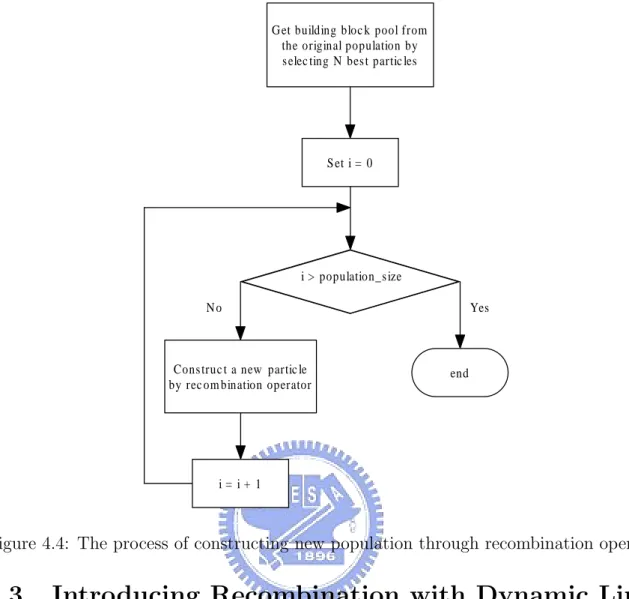
In this study, since we have explicitly identified the linkage group, in order to make good use of linkage information, we design a special recombination operator. The re-combination operator is designed according to the idea of multi-parental rere-combination. In the recombination process, individuals with good fitness are selected and we consider the selected individuals as a building block pool. Every offspring is created by choosing and recombining building blocks from the pool at random. We use this recombination process to generate the whole next population. An illustration of how a new individual is generated is shown as Figure 4.3. By repeating the process shown in Figure 4.3, we can reconstruct a new population in which each particle is composed by the good building blocks. A flowchart of the population reconstructing process is shown in Figure 4.4.
A seemingly similar operator has been proposed by Smith and Fogarty [48]. In [48], the representation on which the recombination operator works takes the form of markers on the chromosome which specify whether or not a gene is linked to its neighbors. Different chromosomes form different numbers of building blocks. However, our recombination operator keeps a global linkage configuration such that every individual in the pool is decomposed into the same building blocks.
BBs po o l BB1 BB2 BB3 BB1 BB2 BB3 BB1 BB2 BB3 BB1 BB2 BB3 ne w individua l ra domly c hoose B B from e a c h individua l BB1 BB2 BB3 individual1 individual2 individual3 individualn BB1 BB2 BB3 BB1 BB2 BB3 . . . individual4 individualn -1
Figure 4.3: The procedure of how a new particle is generated through the recombination operator
In this algorithm, the recombination operator is used to mix building blocks, and to construct a new population. In the beginning of optimization process, this procedure can be viewed as a global search, while the particle swarm optimizer serves as a local searcher that fine tune the building blocks. As the optimization goes on, the population starts to converge and the building blocks become similar. Thus the recombination operator plays as a local searcher at this time. The cooperation between them and the complete flow of this algorithm will be described in the next section.
G et building bloc k pool from the original population by s elec ting N bes t partic les
Cons truc t a new partic le by rec om bination operator
i > population_s ize S et i = 0 i = i + 1 end Yes N o
Figure 4.4: The process of constructing new population through recombination operator
4.3
Introducing Recombination with Dynamic
Link-age Discovery in PSO
The main purpose in this study is to enhance the PSO’s performance by introducing the genetic operator with linkage concept. To achieve this goal, we design the dynamic linkage discovery technique and the corresponding recombination operator. Although there were many variant of the particle swarm optimization proposed in the literature. For the convenience of analyzing and development, in this algorithm, we applied only a modified version of the particle swarm optimization wchich proposed by Shi and Eberhart [17]. A composition of these three components is described in the following paragraph.
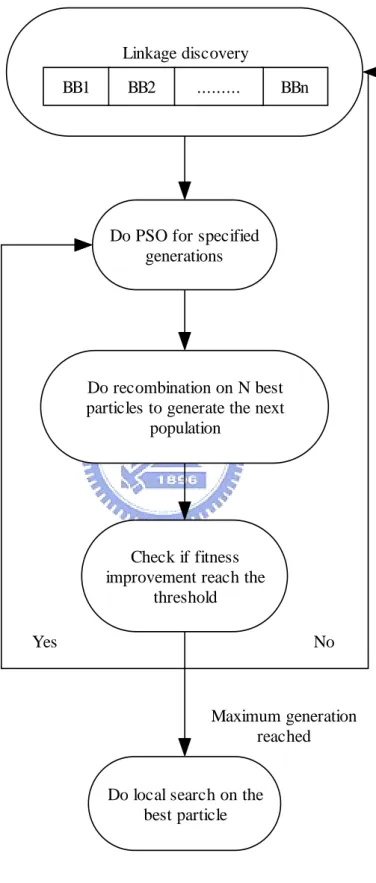
In the proposed algorithm, we repeat the PSO procedure for a certain number of generations, we term such a period a PSO epoch in the rest of this report. After each PSO epoch, we select the N best particles from the population to construct the building block pool and conduct the recombination operation according to the building blocks
identified by dynamic linkage discovery. After the recombination process, the linkage discovery step is executed when necessary. We calculate the average fitness of the current epoch, compare the average with the one calculated during last epoch, and check if the improvement is significant enough. When the specified threshold is reached, the current linkage groups are considered suitable and remain unchanged for the next PSO epoch. Otherwise, it is considered that the building blocks do not work well for the current search stage. Thus, the linkage discovery process restarts, and the linkage configuration is randomly reassigned. The pseudo code and flow of the algorithm are shown in Figures 4.5 and 4.6, respectively.
Similar research works have been done in the literature, such as PSO with learning strategy [23, 24] and PSO with adaptive linkage learning [12]. The main difference be-tween the proposed algorithm and them is that we introduce the recombination operator specifically designed to work with the identified building blocks. In addition, we propose a new linkage discovery technique to dynamically adapt the linkage during the search process.
4.4
Summary
In this chapter, we first described how we deal with the genetic linkages. Based on the natural selection concept, a dynamic linkage discovery technique is designed. This tech-nique is designed to identified the linkage configurations in real-parameter optimization problems. In order to make good use of linkages, we then propose the recombination operator. In this algorithm, we introduce the recombination with genetic linkage concept to particle swarm optimization. As a result, a new optimization algorithm is proposed and numerical experiments are also conducted. The experimental results will be shown and discussed in Chapter 5.
PSO with Recombination Operator & Dynamic Linkage Discovery Step1: Do Finding the linkage group.
1. Generate an integer number N from 1 to D (D: problem dimensions). 2. Assign each dimension an integer number from 1 to N.
3. Dimensions with the same number grouped as the same building block.
Step2: Do PSO algorithm on the population. 1. For each particle
Evaluate fitness value
If the fitness value is better than the best fitness value (pBest) in history set current value as the new pBest
End
2. Choose the particle with the best fitness value of all the particles as the gBest
3. For each particle
Calculate particle’s velocity. Update particle’s position.
End
4. Repeat 1 to 3 until maximum iterations is attained. Step3: Do Recombination to generate next population.
1. Select M best particles from the population. 2. For i = 1 to N (N: number of building blocks) Select ith building block from particles 1 to M.
Put the selected building block to the ith slot of the new generated particle.
End
3. Repeat 2 for S times, S means the swarm size.
Step4: If fitness value improves over the specified threshold, then go to Step2, else go to Step3.
Repeat until the maximum iteration is reached. Step5: Do local search on the best particle.
Linkage discovery
BB1 BB2 ... BBn
Do PSO for specified generations
Do recombination on N best particles to generate the next
population
Check if fitness improvement reach the
threshold
Do local search on the best particle
Yes No
Maximum generation reached
Chapter 5
Experimental Results
Computer simulations are conducted to demonstrate the performance of PSO-RDL. The experiments are focused on the real-valued parameter optimization. The test problems are proposed in the special session on real-parameter optimization in CEC2005 aimed at developing high-quality benchmark functions to be publicly available to the researchers around the world for evaluating their algorithms. The following topics will be covered in this chapter:
• Test Functions: The description of test problems
• Parameter Setting: The parameter settings used in the experiment.
• Experimental Results: Show the numerical results of the experiments as well as the linkage dynamics during optimizing several functions of different characteristics. • Discussion: Discuss the results and observations from the experiments.
5.1
Test Functions
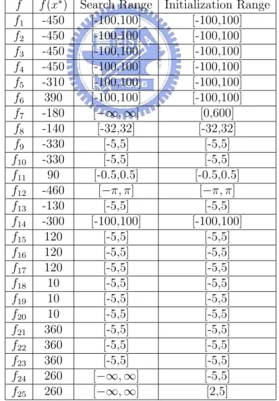
The newly proposed set of test problems includes 25 functions of different characteristics. Five of them are unimodal problems, and others are multimodal problems [49]. A tech-nical report of detail description of test problems is available at
http://nclab.tw/TR/2005/NCL-TR-2005001.pdf. All test functions are tested on 10 dimensions in this study. The summary of the 25 functions is shown as follows:
– F1: Shifted Sphere Function
– F2: Shifted Schewefel’s Problem 1.2
– F3: Shifted Rotated High Conditioned Elliptic Function
– F4: Shifted Schwefel’s Problem 1.2 with Noise in Fitness
– F5: Schwefel’s Problem 2.6 with Global Optimum on Bounds
• Multimodal Functions (20): – Basic Functions (7):
∗ F6: Shifted Rosenbrock’s Function
∗ F7: Shifted Rotated Griewank’s Function without Bounds
∗ F8: Shifted Rotated Ackley’s Function with Global Optimum on Bounds
∗ F9: Shifted Rastrigin’s Function
∗ F10: Shifted Rotated Rastrigin’s Function
∗ F11: Shifted Rotated Weierstrass Function
∗ F12: Schwefels’ Problem 2.13
– Expanded Function (2)
∗ F13: Expanded Extended Griewank’s plus Rosenbrock’s Function (F8F2)
∗ F14: Shifted Rotated Expanded Scaffer’s F6
– Hybrid Composition Function (11) ∗ F15: Hybrid Composition Function
∗ F16: Rotated Hybrid Composition Function
∗ F17: Rotated Hybrid Composition Function with Noise in Fitness
∗ F18: Rotated Hybrid Composition Function
∗ F19: Rotated Hybrid Composition Function with a Narrow Basin for the
Global Optimum
∗ F20: Rotated Hybrid Composition Function with the Global Optimum on
∗ F21: Rotated Hybrid Composition Function
∗ F22: Rotated Hybrid Composition Function with High Condition Number
Matrix
∗ F23: Non-Continuous Rotated Hybrid Composition Function
∗ F24: Rotated Hybrid Composition Function
∗ F25: Rotated Hybrid Composition Function without Bounds
The properties and the formulas of these functions are presented in the appendix A. The bias of fitness value for each function f (x∗), the search ranges [Xmin, Xmax] and the
initializatino range of each function are given in Table 5.1. The individuals of global optimum for each function are given in Table B.1.
Table 5.1: Global optimum, search ranges and initialization ranges of the test functions f f (x∗) Search Range Initialization Range
f1 -450 [-100,100] [-100,100] f2 -450 [-100,100] [-100,100] f3 -450 [-100,100] [-100,100] f4 -450 [-100,100] [-100,100] f5 -310 [-100,100] [-100,100] f6 390 [-100,100] [-100,100] f7 -180 [−∞, ∞] [0,600] f8 -140 [-32,32] [-32,32] f9 -330 [-5,5] [-5,5] f10 -330 [-5,5] [-5,5] f11 90 [-0.5,0.5] [-0.5,0.5] f12 -460 [−π, π] [−π, π] f13 -130 [-5,5] [-5,5] f14 -300 [-100,100] [-100,100] f15 120 [-5,5] [-5,5] f16 120 [-5,5] [-5,5] f17 120 [-5,5] [-5,5] f18 10 [-5,5] [-5,5] f19 10 [-5,5] [-5,5] f20 10 [-5,5] [-5,5] f21 360 [-5,5] [-5,5] f22 360 [-5,5] [-5,5] f23 360 [-5,5] [-5,5] f24 260 [−∞, ∞] [-5,5] f25 260 [−∞, ∞] [2,5]
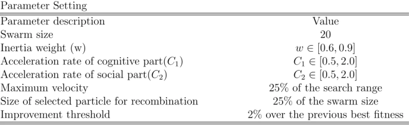
Table 5.2: Parameter setting in this numerical experiments Parameter Setting
Parameter description Value
Swarm size 20
Inertia weight (w) w ∈ [0.6, 0.9] Acceleration rate of cognitive part(C1) C1 ∈ [0.5, 2.0]
Acceleration rate of social part(C2) C2 ∈ [0.5, 2.0]
Maximum velocity 25% of the search range Size of selected particle for recombination 25% of the swarm size Improvement threshold 2% over the previous best fitness
Numerical test problems described above were simulated to evaluate the performance of the proposed algorithm. This benchmark with multiple types of functions such as unimodal, multimodal, expanded and composition functions, so that the strength and weakness of the algorithm could be analyzed comprehensively.
5.2
Parameter Setting
The parameter setting in this study is described as follows:
The number of particles is set to 20, 0.6 ≤ w ≤ 0.9, 0.5 ≤ ~ϕ1 ≤ 2.0, 0.5 ≤ ~ϕ2 ≤ 2.0,
and Vmax restricts the particles’ velocity, where Vmax is equal to 25% of the initialization
range. N , the number of particles selected for the recombination, is set to 25% of the swarm size. The threshold which decides if the linkage configuration should be changed is set to 2% of the previous best fitness value. A list of the parameter setting is shown in Table 5.2.
5.3
Experimental Results
The complete experimental results are listed in Tables 5.3, 5.4, 5.5, 5.6 and 5.7. According to the definition in the special session, PSO-RDL successfully solved problems 1, 2, 4, 5, 6, 7 and 12 in the experimental results. Moreover, comparable results are achieved in solving problems 3, 8, 11, 13 and 14. Unfortunately, PSO-RDL failed to solve problems 9, 10 and 15-25. Table 5.8, 5.9 , 5.10, 5.11 and 5.12 show the experimental results compared with other evolutionary algorithms proposed in the special session. Table 5.13 gives the
number of successfully solved problems. From these comparisons, it can be observed that PSO-RDL has a good performance for most problems. Table C.1 shows the solution found by PSO-RDL for each function in this benchmark. Figures 5.1, 5.2, 5.3 and 5.4 show how the dynamic linkage discovery technique changes the linkage configuration during the optimization process. Detailed discussion on the experimental results is presented in the next section.
5.4
Discussion
From the experimental results listed in Table 5.3, it can be considered that the proposed algorithm is able to provide good results for the benchmark. The first five functions are unimodal functions. Function 1 is shifted sphere function, Function 2 is shifted Schwefel’s problem 1.2, and Function 3 is shifted rotated high condition elliptic function. These three functions have different condition numbers which make Function 3 much harder than Functions 1 and 2. Function 4 is shifted Schwefel’s problem 1.2 with noise in fitness. Function 5 is Schwefel’s problem 2.6 with global optimum on bounds. From the results, we can observe that PSO-RDL reaches the predefined error tolerance level for Functions 1, 2, 4, and 5. For Function 3, PSO-RDL achieves an error of 1e-4 but does not meet the 1e-6 criterion. It may be caused by the multiplicator 106 in the objective function
which greatly amplifies the error. In summary, PSO-RDL provides a sufficiently good performance for the unimodal functions in this benchmark.
Functions 6-14 are multimodal problems. Function 6 is shifted Rosenbrock’s function, a problem with a very narrow valley from the local optimum to the global optimum, and solved by PSO-RDL. Function 7 is shifted rotated Griewank’s function without bounds, and this function makes the search easily away from the global optimum. Fortunately, PSO-RDL solved it twice in 25 trials and can achieve a comparable result in average for this function. Function 8 is shifted rotated Ackley’s function with global optimum on bounds, which has a very narrow global basin and half of the dimensions of this basin are on the boundaries. Hence, the search algorithm cannot easily find the global basin when the recombination operator is used. The PSO-RDL failed on this problem in all 25
FES 1 2 3 4 5 1st( M in) 5 .69 75 E -02 2.3 397 E+01 4.8 24 4E+0 5 1.6 83 9E+0 2 1.1 41 0E+0 0 7t h 2.20 13 E+00 1.5 546 E+02 1.3 21 5E+0 6 8.4 54 1E+0 2 1 .138 9E+0 1 13 th(Median) 1.25 39 E + 01 2.99 70 E+02 2.0 604 E+06 2.4 96 6E+0 3 3.4 23 0E+0 1 1E+ 03 19 th 1.0 87 8E+0 2 5 .883 5E+0 2 3 .653 2E+ 06 4 .99 21E+ 03 1 .37 66 E + 03 25 th(Max ) 6.4 91 2E+0 2 7.7 40 4E+0 3 8 .658 0E+0 7 1 .869 5E+ 04 9 .46 77E+ 03 mean 1 .171 1E+ 02 9 .89 02E+ 02 7 .44 99 E + 06 4.34 45 E + 03 1.7 836 E+03 Std 2 .042 5E+0 2 1 .70 74E+ 03 1 .76 30E+ 07 5.28 37 E + 03 3.21 11 E+03 1st( M in) 0.00 00 E+00 1.86 05 E -10 1.9 32 7E+0 4 6.3 92 8E+0 0 0.0 00 0E+0 0 7t h 5 .68 43 E -14 5.18 10 E -09 4.9 19 7E+0 4 1.1 92 2E+0 2 0 .000 0E+0 0 13 th(Median) 5 .68 43E-14 4 .05 01 E -08 1.0 152 E+05 4.2 55 7E+0 2 1.2 733 E-1 0 1E+ 04 19 th 1.1 369 E-1 3 9.8 91 8E-0 8 1 .742 7E+ 05 9 .03 10E+ 02 2 .01 35E-07 25 th(Max ) 1.0 800 E-1 2 5.6 686 E-0 7 6 .751 8E+0 5 1 .537 6E+ 04 4 .557 0E-04 mean 1.7 05 3E-13 7 .940 2E-08 1 .56 10 E + 05 1.41 38 E + 03 2 .31 91 E -05 Std 2.5 52 7E-1 3 1 .204 9E-07 1 .71 42 E + 05 3.18 80 E + 03 9 .29 21 E -05 1st( M in) 0.00 00 E+00 5.68 43 E -14 3.81 07 E-0 4 1.4 211 E-1 2 0.0 00 0E+0 0 7t h 0.00 00 E+00 5.68 43 E -14 4.6 282 E-0 4 5.5 718 E-1 0 0 .000 0E+0 0 13 th(Median) 0.00 00 E + 00 1 .13 69 E -13 4.72 32 E -04 4.3 663 E-0 9 0.0 00 0E+0 0 1E+ 05 19 th 5.6 843 E-1 4 1.7 05 3E-1 3 4.7 23 6E-04 1 .818 4E-08 3 .63 80E-12 25 th(Max ) 5.6 843 E-1 4 7.9 581 E-1 3 1 .236 0E+0 0 3.3 32 9E-06 2 .610 0E-06 mean 2.5 01 1E-14 1 .773 5E-13 9 .68 48E-02 2 .46 86E-07 2 .09 43 E -07 Std 2.8 79 8E-1 4 2 .031 8E-13 3 .337 5E-01 7 .07 12E-07 7 .22 48 E -07 T a ble 5 .3: B est functio n err or v a lues ac hiev ed whe n FES = 1e+ 3, 1 e+4, and 1e+5 for functions 1-5. The predefined erro r is 1e-6 fo r the se fiv e functions. These functio ns a re all unimo da l problems, and PSO -R DL suc cessf ully so lv ed func tions 1, 2 , 4, a nd 5 . Compa rable results for function 3 w ere o bta ine d.
FES 6 7 8 9 10 1st( M in) 3.79 57 E+01 1.2 672 E+03 2.0 47 7E+0 1 1.6 20 8E+0 1 1.8 93 7E+0 1 7t h 1.24 97 E+03 1.2 672 E+03 2.0 59 9E+0 1 2.8 01 4E+0 1 4 .058 6E+0 1 13 th(Median) 1.04 55 E + 04 1.26 78 E+03 2.0 703 E+01 3.0 17 2E+0 1 4.9 84 7E+0 1 1E+ 03 19 th 2.4 27 3E+0 5 1 .286 5E+0 3 2 .075 1E+ 01 4 .33 07E+ 01 5 .95 70 E + 01 25 th(Max ) 2.6 04 7E+0 6 1.9 41 9E+0 3 2 .099 1E+0 1 6 .580 8E+ 01 7 .08 26E+ 01 mean 3 .921 1E+ 05 1 .34 63E+ 03 2 .07 08 E + 01 3.49 92 E + 01 5.0 378 E+01 Std 7 .724 4E+0 5 1 .62 89E+ 02 1 .195 5E-01 1.36 68 E + 01 1.36 04 E+01 1st( M in) 5 .50 79 E -09 5.18 71 E -01 2.0 00 8E+0 1 3.9 79 8E+0 0 1.5 91 9E+0 1 7t h 3 .54 02 E -02 9.16 88 E -01 2.0 02 2E+0 1 1.5 91 9E+0 1 2 .089 4E+0 1 13 th(Median) 1.64 79 E + 00 9 .59 36 E -01 2.0 070 E+01 2.3 87 9E+0 1 3.5 81 8E+0 1 1E+ 04 19 th 1.1 23 6E+0 2 9.9 95 6E-0 1 2 .009 3E+ 01 2 .98 49E+ 01 5 .47 22 E + 01 25 th(Max ) 5.8 17 9E+0 2 1.3 72 3E+0 0 2 .028 2E+0 1 6 .566 7E+ 01 6 .96 47E+ 01 mean 8 .701 2E+ 01 9 .729 9E-01 2 .00 84 E + 01 2.39 33 E + 01 3.8 564 E+01 Std 1 .654 9E+0 2 1 .834 5E-01 7 .734 0E-02 1.26 93 E + 01 1.79 76 E+01 1st( M in) 1 .27 84 E -10 1.69 93 E -10 2.0 00 0E+0 1 1.9 89 9E+0 0 1.5 91 9E+0 1 7t h 9 .05 80 E -10 1.47 80 E -02 2.0 00 0E+0 1 7.9 59 7E+0 0 2 .089 4E+0 1 13 th(Median) 2 .99 76E-09 4 .92 57 E -02 2.0 000 E+01 1.0 94 5E+0 1 3.5 81 8E+0 1 1E+ 05 19 th 2.6 304 E-0 7 1.0 57 7E-0 1 2 .000 0E+ 01 1 .69 14E+ 01 5 .47 22 E + 01 25 th(Max ) 3.9 86 6E+0 0 1.5 520 E-0 1 2 .000 1E+0 1 3 .681 3E+ 01 6 .96 47E+ 01 mean 9.5 67 8E-01 5 .731 6E-02 2 .00 00 E + 01 1.24 97 E + 01 3.8 564 E+01 Std 1 .737 7E+0 0 4 .660 0E-02 2 .168 5E-04 8.17 48 E + 00 1.79 76 E+01 T a ble 5 .4: Bes t functio n err or v alues a chiev ed whe n FES = 1e+ 3, 1e+ 4, a nd 1 e+5 for functio ns 6 -1 0. The predefined err or is 1 e-2 fo r these fiv e functio ns. The funct ions are all m ult imo dal pro blems , and PSO-RDL succes sfully solv ed functio n 6 and ga v e compa rable results on functions 7 and 8 . Ho w ev er , w o rse results w ere obt ained o n functio ns 9 a nd 1 0 due to the lar ge n um b er o f lo ca l o ptima.
FES 1 1 1 2 1 3 1 4 15 1st( M in) 5.72 83 E+00 1.5 379 E+02 1.5 40 2E+0 0 3.4 97 2E+0 0 2.2 39 7E+0 2 7t h 6.80 54 E+00 9.7 877 E+02 2.8 68 0E+0 0 3.9 30 0E+0 0 3 .178 5E+0 2 13 th(Median) 8.21 36 E + 00 6.85 87 E+03 3.3 114 E+00 4.1 02 5E+0 0 4.1 72 0E+0 2 1E+ 03 19 th 9.3 26 0E+0 0 1 .777 0E+0 4 4 .052 3E+ 00 4 .15 70E+ 00 4 .94 06 E + 02 25 th(Max ) 9.8 27 1E+0 0 3.8 00 7E+0 4 4 .907 6E+0 0 4 .453 7E+ 00 7 .50 28E+ 02 mean 8 .058 9E+ 00 1 .07 18E+ 04 3 .32 69 E + 00 4.02 85 E + 00 4.2 130 E+02 Std 1 .237 7E+0 0 1 .15 50E+ 04 8 .400 3E-01 2 .31 82E-01 1.32 74 E+02 1st( M in) 2.87 33 E+00 9.10 41 E -05 3.75 07 E-0 1 3.2 02 7E+0 0 1.2 40 8E+0 2 7t h 4.86 07 E+00 4.16 26 E -01 7.4 933 E-0 1 3.6 31 1E+0 0 2 .699 6E+0 2 13 th(Median) 5.42 40 E + 00 6.94 68 E+00 1.1 691 E+00 3.8 06 2E+0 0 3.5 15 1E+0 2 1E+ 04 19 th 6.6 47 3E+0 0 2 .725 2E+0 1 1 .624 7E+ 00 4 .02 19E+ 00 4 .58 82 E + 02 25 th(Max ) 9.0 39 2E+0 0 1.6 93 6E+0 3 8.9 95 3E-0 1 4 .411 2E+ 00 6 .05 97E+ 02 mean 5 .758 5E+ 00 1 .59 10E+ 02 1 .19 72 E + 00 3.79 81 E + 00 3.5 718 E+02 Std 1 .520 0E+0 0 4 .47 50E+ 02 5 .774 2E-01 3 .29 71E-01 1.31 33 E+02 1st( M in) 2.82 87 E+00 1.09 67 E -09 3.38 23 E-0 1 3.1 35 9E+0 0 1.0 06 5E+0 2 7t h 4.85 24 E+00 4.91 12 E -09 6.1 622 E-0 1 3.5 81 2E+0 0 1 .378 6E+0 2 13 th(Median) 5.42 29 E + 00 7 .59 48 E -08 7.49 10 E -01 3.8 06 0E+0 0 2.0 85 7E+0 2 1E+ 05 19 th 5.9 53 7E+0 0 4.4 37 6E-0 6 1 .111 9E+ 00 4 .01 37E+ 00 4 .29 23 E + 02 25 th(Max ) 9.0 39 2E+0 0 1.6 93 6E+0 3 1 .985 1E+0 0 4 .410 8E+ 00 6 .05 96E+ 02 mean 5 .575 4E+ 00 1 .31 25E+ 02 8 .87 32E-01 3.77 96 E + 00 2.7 113 E+02 Std 1 .416 1E+0 0 4 .50 06E+ 02 4 .060 1E-01 3 .43 64E-01 1.58 81 E+02 T a ble 5.5 : Be st func tion erro r v alues a chie v ed when FES = 1e+3 , 1e+4 , and 1e+5 for func tions 11 -1 4. The predefined erro r is 1e-2 fo r these fo ur functio ns. T he functions are all m ult imo dal pro blems , a nd functio ns 1 3 and 1 4 are extended func tions. P SO -RDL succe ssfully solv ed function 12 a nd o bta ine d compa rable results o n function s 11 , 1 3, and 14 .
FES 1 6 1 7 1 8 1 9 20 1st( M in) 1.39 47 E+02 1.4 536 E+02 8.0 04 9E+0 2 8.0 27 0E+0 2 8.2 37 0E+0 2 7t h 1.88 25 E+02 2.1 723 E+02 1.0 16 3E+0 3 9.9 13 3E+0 2 9 .749 0E+0 2 13 th(Median) 2.23 34 E + 02 2.51 07 E+02 1.0 489 E+03 1.0 18 0E+0 3 1.0 23 0E+0 3 1E+ 03 19 th 2.5 10 6E+0 2 2 .893 9E+0 2 1 .131 3E+ 03 1 .08 36E+ 03 1 .05 24 E + 03 25 th(Max ) 9.9 56 0E+0 2 7.1 13 9E+0 2 1 .199 1E+0 3 1 .117 8E+ 03 1 .12 51E+ 03 mean 2 .576 6E+ 02 2 .76 83E+ 02 1 .04 89 E + 03 1.01 02 E + 03 9.9 493 E+02 Std 1 .738 2E+0 2 1 .14 60E+ 02 1 .05 00E+ 02 8.72 27 E + 01 8.69 21 E+01 1st( M in) 1.27 82 E+02 1.1 722 E+02 8.0 00 0E+0 2 6.9 57 8E+0 2 8.0 00 0E+0 2 7t h 1.50 93 E+02 1.5 412 E+02 9.8 80 0E+0 2 9.7 80 5E+0 2 8 .369 5E+0 2 13 th(Median) 1.73 54 E + 02 1.83 04 E+02 1.0 367 E+03 1.0 13 4E+0 3 1.0 09 0E+0 3 1E+ 04 19 th 2.1 74 4E+0 2 2 .203 6E+0 2 1 .118 2E+ 03 1 .05 17E+ 03 1 .04 16 E + 03 25 th(Max ) 9.8 80 7E+0 2 5.9 98 9E+0 2 1 .195 6E+0 3 1 .108 4E+ 03 1 .10 05E+ 03 mean 2 .202 8E+ 02 2 .08 32E+ 02 1 .02 48 E + 03 9.90 23 E + 02 9.6 112 E+02 Std 1 .738 8E+0 2 1 .00 39E+ 02 1 .21 07E+ 02 1.02 72 E + 02 1.05 17 E+02 1st( M in) 1.27 82 E+02 1.1 866 E+02 8.0 00 0E+0 2 6.9 52 6E+0 2 8.0 00 0E+0 2 7t h 1.50 93 E+02 1.6 793 E+02 9.8 80 0E+0 2 9.7 67 4E+0 2 8 .243 6E+0 2 13 th(Median) 1.73 42 E + 02 2.11 70 E+02 1.0 362 E+03 1.0 02 1E+0 3 1.0 09 0E+0 3 1E+ 05 19 th 2.1 63 5E+0 2 2 .365 5E+0 2 1 .118 2E+ 03 1 .04 80E+ 03 1 .04 13 E + 03 25 th(Max ) 9.8 63 2E+0 2 6.1 46 8E+0 2 1 .190 5E+0 3 1 .108 4E+ 03 1 .10 02E+ 03 mean 2 .195 8E+ 02 2 .22 22E+ 02 1 .02 27 E + 03 9.84 99 E + 02 9.5 905 E+02 Std 1 .735 0E+0 2 1 .00 19E+ 02 1 .18 83E+ 02 1.01 89 E + 02 1.05 67 E+02 T a ble 5 .6: B est fu nc tion error v alu es ac hiev ed when FE S = 1e+3 , 1e+ 4, a nd 1e+5 fo r fu nc tions 16-20 . The predefine d erro r is 1 e-2 fo r F unc tion 16 a nd 1 e-1 for the other four functions.
FES 2 1 2 2 2 3 2 4 25 1st( M in) 5.00 26 E+02 7.8 706 E+02 5.5 40 1E+0 2 8.1 57 3E+0 2 1.7 34 2E+0 3 7t h 1.05 61 E+03 9.1 841 E+02 1.1 41 9E+0 3 9.7 92 8E+0 2 1 .749 1E+0 3 13 th(Median) 1.22 17 E + 03 9.56 52 E+02 1.2 438 E+03 1.0 24 3E+0 3 1.7 68 2E+0 3 1E+ 03 19 th 1.2 71 3E+0 3 9 .986 0E+0 2 1 .285 0E+ 03 1 .26 37E+ 03 1 .79 93 E + 03 25 th(Max ) 1.2 81 4E+0 3 1.0 63 3E+0 3 1 .326 4E+0 3 1 .332 5E+ 03 1 .95 82E+ 03 mean 1 .080 5E+ 03 9 .49 73E+ 02 1 .11 32 E + 03 1.07 96 E + 03 1.7 934 E+03 Std 2 .723 3E+0 2 7 .82 69E+ 01 2 .73 59E+ 02 1.60 30 E + 02 6.57 46 E+01 1st( M in) 3.00 00 E+02 7.5 236 E+02 4.2 51 7E+0 2 5.0 00 0E+0 2 1.7 16 4E+0 3 7t h 1.04 50 E+03 8.2 582 E+02 1.1 41 7E+0 3 5.0 45 6E+0 2 1 .729 0E+0 3 13 th(Median) 1.15 82 E + 03 9.12 75 E+02 1.2 197 E+03 9.6 49 1E+0 2 1.7 40 1E+0 3 1E+ 04 19 th 1.1 89 9E+0 3 9 .339 7E+0 2 1 .259 4E+ 03 1 .11 42E+ 03 1 .74 78 E + 03 25 th(Max ) 1.2 65 8E+0 3 1.0 20 9E+0 3 1 .319 5E+0 3 1 .288 3E+ 03 1 .87 27E+ 03 mean 9 .979 5E+ 02 8 .91 47E+ 02 1 .08 74 E + 03 8.89 51 E + 02 1.7 452 E+03 Std 3 .301 6E+0 2 7 .07 07E+ 01 2 .92 07E+ 02 3.03 72 E + 02 2.94 65 E+01 1st( M in) 3.00 00 E+02 7.5 022 E+02 4.2 51 7E+0 2 2.0 00 0E+0 2 1.7 37 2E+0 3 7t h 1.04 50 E+03 8.0 458 E+02 1.1 41 7E+0 3 5.0 00 0E+0 2 1 .749 5E+0 3 13 th(Median) 1.15 82 E + 03 9.10 47 E+02 1.1 881 E+03 5.0 46 2E+0 2 1.7 55 4E+0 3 1E+ 05 19 th 1.1 87 8E+0 3 9 .332 4E+0 2 1 .257 8E+ 03 1 .02 13E+ 03 1 .76 47 E + 03 25 th(Max ) 1.2 64 7E+0 3 1.0 18 9E+0 3 1 .284 6E+0 3 1 .299 5E+ 03 1 .80 87E+ 03 mean 9 .942 9E+ 02 8 .86 66E+ 02 1 .07 76 E + 03 7.20 04 E + 02 1.7 588 E+03 Std 3 .274 9E+0 2 7 .11 76E+ 01 2 .86 81E+ 02 3.96 39 E + 02 1.54 16 E+01 T a ble 5 .7: B est fu nc tion error v alu es ac hiev ed when FE S = 1e+3 , 1e+ 4, a nd 1e+5 fo r fu nc tions 21-25 . The predefine d erro r is 1 e-1 fo r these four functio ns .