DESIGN OF DISCRETE TIME CONTROLLER — STATE SPACE APPROACH

(1)

DESIGN OF DISCRETE TIME CONTROLLER —

STATE SPACE APPROACH

LECTURE 8

(2)

OUTLINE

•

State Feedback

•

Pole (eigenvalue) placement, when can it be done?

•

Deadbeat control

•

Other issues (input scaling, observability)

•

Comparison with output feedback

•

Observer design

(3)

STATE SPACE DESIGN State Space Design

• Work with State Space Equations

• Less “graphical”, more computational (eigenvalue, norm, cost function)

• Mostly result in full-state feedback algorithms

Continuous-Time Systems Discrete-Time Systems

( ) ( ) ( )

x A x B u

y C x D u

t t t

= ⋅ + ⋅

x A x B u

y C x D u

( ) ( ) ( )

k k k

+ = ⋅ + ⋅

= ⋅ + ⋅

1 : 1 : 1

: 1

x n

u r

y m

×

(4)

STATE FEEDBACK State Feedback

• Assumes that all the state variables are available (from direct measurement,

estimation, observation, etc.) .

Continuous-Time Systems Discrete-Time Systems ( ) t = − ⋅ K ( ) t + ⋅ N r ( ) t

u x u ( ) k = − ⋅ K x ( ) k + ⋅ N r ( ) k

state feedback gain feedforward gain

( )

( ) ( ) ( )

t t r t

= − ⋅ + ⋅

x A BK x BN y C DK x DN

( )

( 1) ( ) ( )

( ) ( ) ( )

k k r k

+ = − ⋅ + ⋅

= − ⋅ + ⋅

x A BK x BN

y C DK x DN

(5)

STATE FEEDBACK (CONT.) State Feedback (cont.)

q

⁻¹

u(k)

A

C B

D

y(k) x(k) +

+ +

+

x(k+1)

-K

r(k)

+ +

Open-Loop Plant

N

Note: the feedback law is usually written as in the literature. This is based on the assumption of a "regulation"

problem. In other words, the output y is controlled to stay close to zero. The configuration above is for a general

(tracking) problem where the reference signal r may not be zero.

u = − ⋅ K x

(6)

POLE PLACEMENT THROUGH STATE FEEDBACK

Pole Placement (Eigenvalue Assignment) Through State Feedback

( )

( ) ( ) ( )

t t r t

= − ⋅ + ⋅

x A BK x BN y C DK x DN

( )

( 1) ( ) ( )

( ) ( ) ( )

k k r k

+ = − ⋅ + ⋅

= − ⋅ + ⋅

x A BK x BN

y C DK x DN

Fact: If (A,B) is in controllable canonical form, pole placement is possible If (A,B) controllable, can be transformed to CCF, pole placement is possible.

x k x k

x k

x k a a a a

x k x k

u k

n

n n n n

n n 1

2

1

1 2 1

1 2

1

1 1

0 1 0 0

0 0 1 0

0 0 0 1

( )

( ) ( )

( ) +

+ + +

L N MM MM MM

O Q PP PP

PP ⁼ ⁻ ⁻ ⁻ ⁻

L N MM MM MM

O Q PP PP PP

L N MM MM MM

O Q PP PP PP ⁺

L N MM MM MM

O Q PP PP PP ^⋅

−

− −

−

[

1 2 1

]

1 1 2 1

( ) ( ) ( )

( ) ( ) ( ) ( )

n n n

u k k k k k k N r k

k x k k x k k x k N r k

− −

−

= − ⋅ + ⋅

= − ⋅ − ⋅ − − ⋅ + ⋅

x

(7)

POLE PLACEMENT (CONT.) Pole Placement (cont.)

1 2 1

0 1 0 0

0 0 1 0

( 1) ( ) ( )

0 0 0 1

(

_n _n

) (

_n _n

) (

_n _n

) ( )

k k BN r k

a a a a

k k

₋ ₋

k

₋ ₋

k

⎡ ⎤

⎢ ⎥

+ = ⎢ ⎥ + ⋅

⎢ ⎥

⎢ − + − + − + − + ⎥

⎣ ⎦

x x

x k x k

x k

x k a a a a

x k x k

x k x k

u k

n

n n n n

n n 1

2

1

1 2 1

1 2

1

1 1

0 1 0 0

0 0 1 0

0 0 0 1

0 0

0 1

( )

( ) ( )

( ) +

+

+ +

L N MM MM MM

O Q PP PP

PP

⁼ − − − −

L N MM MM MM

O Q PP PP PP

L N MM MM MM

O Q PP PP PP

⁺

L N MM MM MM

O Q PP PP PP

^⋅

−

− −

−

[

1 2 1

]

1 1

1 2

( ) ( ) ( )

( ) ( ) ( ) ( )

n n n

u k k N r k

x k x k x k N r

k k k k

− −

−

= − ⋅ + ⋅

= − ⋅ − ⋅ − − ⋅ + ⋅

x

( ₁ ₁ ) ¹ ( ₂ ₂ ) ² ( ) ⁰

n n

n n n

z + k + a z ⁻ + k + a z ⁻ + + k + a =

Closed-loop char. eq.

(8)

EX8.1 STATE FEEDBACK POLE PLACEMENT Ex8.1 State Feedback Pole Placement

0 1 0

x x 1

d k b f

x x

dt m m m

⎡ ⎤ ⎡ ⎤

⎡ ⎤ = ⎢ − − ⎥ ⎡ ⎤ + ⎢ ⎥

⎢ ⎥ ⎢ ⎥ ⎢ ⎥ ⎢ ⎥

⎣ ⎦ ⎣ ⎦ ⎣ ⎦ ⎣ ⎦

[ ]

2 1 2 1

1 2 2 1 2

1 0 1

det det 1 [ ] det

0 s s

s k b k k k k b k

s s

m m m m m

b k k k b k k k

s s s s

m m m m

⎡ ⎡ − ⎤ ⎡ ⎤ ⎤ ⎡ − ⎤

⎢ ⎢ ⎥ ⎢ ⎥ ⎥ ⎢ ⎥

− + = ⎣ ⎢ ⎢ ⎢ ⎣ ⎢ + ⎦ ⎣ ⎦ ⎥ ⎢ ⎥ ⎥ ⎢ ⎥ + ⎥ ⎦ ⎥ = ⎢ ⎢ ⎣ + + + ⎥ ⎥ ⎦

+ + + +

⎛ ⎞

= ⎜ + ⎟ + = + + =

⎝ ⎠

I A BK

State feedback:

If the desired locations of the closed-loop poles are and ⁻ ^α

₁

⁻ ^α

₂

b k

m k m b

k k

m k m k

+ = + ⇒ = + −

+ = ⇒ = −

1 1 2 1 1 2

2 1 2 2 1 2

α α α α

( )

(9)

MATLAB COMMANDS MATLAB commands

» help place

PLACE Pole placement technique

K = PLACE(A,B,P) computes a state-feedback matrix K such that the eigenvalues of A-B*K are those specified in vector P.

No eigenvalue should have a multiplicity greater than the number of inputs.

[K,PREC,MESSAGE] = PLACE(A,B,P) returns PREC, an estimate of how

closely the eigenvalues of A-B*K match the specified locations P (PREC measures the number of accurate decimal digits in the actual

closed-loop poles). If some nonzero closed-loop pole is more than 10% off from the desired location, MESSAGE contains a warning message.

REFERENCE INPUT SCALING Reference Input Scaling

State feedback can change the characteristic polynomial of

the system, therefore, the steady state gain of the closed-loop system is changed. It is necessary to adjust feedforward gain N.

Usually the feedforward gain N is selected to make the overall closed-loop system steady-state gain equals to one.

q⁻¹ u(k)

A

C B

D

y(k) x(k)

+

+ +

+

x(k+1)

-K

r(k)

+ +

Open-Loop Plant

N

(11)

REFERENCE INPUT SCALING

Reference Input Scaling (cont.)

( ) ( ) ( )

( ) ( )

x A x b

C x

t t u t

y t t

= ⋅ + ⋅

= ⋅

For a strictly causal, SISO system

x A x b

C x

( ) ( ) ( )

( ) ( )

k k u k

y k k

+ = ⋅ + ⋅

= ⋅ 1

Continuous-Time Systems Discrete-Time Systems

Closed-loop (from r to y)

G

_CL

( ) s = C I A BK B s − +

⁻¹

⋅ N ^G

_CL

^{( )} ^z ⁼ ^{C I A BK B} ^z ^{− +}

⁻¹

^⋅ ^N

[ ]

( )

[ ]

1 1

1

1 N B B

B B

− −

−

= − +

C A K

[ ]

( )

[ ]

1 1

1

1 N B B

B B

− −

−

= − +

C I A K C I A K

u ( ) t = − ⋅ K x ( ) t + ⋅ N r ( ) t u ( ) k = − ⋅ K x ( ) k + ⋅ N r ( ) k

(12)

EXAMPLE FB/FF SIMULATIONS Example FB/FF Simulations

1

2

2 ( 1) ( ) ( )

0 1

T T

k k u k

T

⎡ ⎤

+ = ⎢ ⎥ + ⎢ ⎥

⎣ ⎦ ⎣ ⎦

x x u k ( ) = − k

₂

k

₁

⋅ x ( ) k

k T p p

1 1 2

2 2 1 2

1 2 3 1 1

= + −

= + +

( )

Desired char. eq.

z

²

+ p z

₁

+ p

₂

= 0

p T e

p e

n ⁿ

n

T

T 1

2

2 1

= − − ⋅

=

−

cos * *

^*

*

ω

^ω

ω

ζ

^ζ

ζ

∗

e j

Pole selection

*

* 0.7 2.0 0.1

n

T

ω

ζ =

=

1 2

1.721 0.7558 p

p

= −

=

1 2

2.616 3.4772 k

k

=

(13)

EXAMPLE (CONT.)

Example FB/FF Simulations (cont.)

0 1 2 3 4 5

0 0.2 0.4 0.6 0.8 1 1.2

Output

No scaling

0 1 2 3 4 5

0 0.2 0.4 0.6 0.8 1 1.2

Output

With scaling

yd yd y

y

t t

r(k) z

1

Unit Delay

K N K

D

Clock

K C

K B

K A

K

-K C:\Teaching\ME561\Notes_Fall2004\MATLABLecture12_pole_placement

(14)

DEADBEAT (FINITE SETTLING TIME) CONTROL Deadbeat (Finite Settling Time) Control

All the closed-loop poles are placed at the origin, i.e., closed-loop char. eq.

z ⁿ = 0

No matter how large the initial condition x(0) may be, the system will be brought to the origin in n steps.

Proof: _x ₍ _k + = 1 _{) (} _{A BK x} − _{) ( )} ⋅ _k

From the Cayley-Hamilton theorem, we have ( A BK − )

ⁿ

= 0

x ( ) ( n = A BK − )

ⁿ

⋅ x ( ) 0 = 0

(15)

EX8.4 DEADBEAT CONTROL Ex8.4 Deadbeat Control

1

2

2 ( 1) ( ) ( )

0 1

T T

k k u k

T

⎡ ⎤

+ = ⎢ ⎥ + ⎢ ⎥

⎣ ⎦ ⎣ ⎦

x x

u k ( ) = − k

₂

k

₁

⋅ x ( ) k

Desired char. eq.

z

²

+ p z

₁

+ p

₂

= 0 ^k T p p

k T p p

1 1 2

2 2 1 2

1 2 3 1 1

= + −

= + +

( )

Deadbeat:

k T k

1 2

T

2

3 2

= and = 1

x ( k ) x ( ) A x ( ) T

T

k

_CL

k

+ = − −

L N MM M

O Q PP

P ⁼ ^⋅

1

1 2 4

1 1

2

1 1

2 4 2 4

1 1 1 1

2 2

CL

T T

⎡ ⎤ ⎡ ⎤

⎢ ⎥ ⎢ ⎥

= ⎢ ⎢ ⎣ ⎢ − − ⎥ ⎢ ⎥ ⎢ ⎦ ⎣ ⎥ ⎢ − − ⎥ ⎥ ⎥ ⎦ =

A 0

(16)

OTHER ISSUES Other Issues

• Controllability is not influenced by state feedback

(assumption: N is non-singular)

• Observability may be lost,

– Why?

– Why do we care?

Rank Rank

Rank

n

W B AB A B A B

BN A BK BN A BK BN A BK BN

b g

C

e j

=

= − − −

−

( ( (

2 1

) ) )

(17)

OUTPUT FEEDBACK Output Feedback

= − ⋅ + ⋅ u K y N r

x A x b

C x

( ) ( ) ( )

( ) ( )

k k u k

y k k

+ = ⋅ + ⋅

= ⋅ 1

Each “K” can be thought as resulting in one DOF on the root locus.

1 1

2 2

0 1 0

1 ( )

x x

d u t

x k m b m x m

dt

⎡ ⎤ ⎡ ⎤ ⎡ ⎤ ⎡ ⎤

= + ⋅

⎢ ⎥ ⎢ ⎣ − − ⎥ ⎦ ⎢ ⎥ ⎢ ⎣ ⎥ ⎦

⎣ ⎦ ⎣ ⎦

u t *( ) = − ⋅ k x t ₁ ₁ ( ) − ⋅ k x t ₂ ₂ ( )

(18)

CLOSED-LOOP (LUENBERGER) OBSERVER

ME561 Lecture 13- 6

Closed-Loop (Luenberger) Observer

An obvious weakness of the open-loop observer is that it did not use the system output, which includes extensive

information about the system states.

Luenberger Observer:

( ) ( ) ( ) ( ) ( )

x k + = ⋅ 1 A x k + ⋅ B u k + ⋅ L y k − ⋅ C x k

q⁻¹

A

+ B + ( )

x k ^{x k}⁽ ⁺¹⁾ C

L +

- +

u(k) q⁻¹

A

C ^x(k) B

y(k) +

+

x(k+1)

u(k)

Original System

Full-Order Observer ( )

y k

q⁻¹

A

+ B + ( )

x k ^{x k}⁽ ⁾

+1

u(k) q⁻¹

A

C ^x(k) B

y(k) +

+

x(k+1)

u(k)

Original System

Open-loop Observer

(19)

POLE PLACEMENT FOR LUENBERGER OBSERVERS Pole Placement for Luenberger Observers

• If the linear time-invariant system (A, C) is observable, eigenvalues of A

_FO

=A-LC can be arbitrarily assigned—

dual property of full state feedback pole placement problem

x k x k

x k x k

a a

x k x k

x k x k

b

n n

n

k k

1 2

1

2 1

1 2

1

1 1

0 0 0 0

1 0 0 0

0 0 1 0

0 0 0 1

1

( ) ( )

+ +

L N MM MM MM

O Q PP PP PP

⁼

−

L N MM MM MM

O Q PP PP PP

L N MM MM MM

O Q PP PP PP

⁺

−

+

x_O A_O x_O

b

b b

u k

y k k

n−

L N MM MM MM

O Q PP PP PP

^⋅

= ⋅

1

2 1

0 0 0 1

B

C

x

O

( )

( ) ( )

[ ]

1 1

2 1 2

1

1 2 1

2

1 1

0 0 0 0

1 0 0 0

0 0 0 1

0 0 1 0

0 0 0 1

n n

L a L

a

L a L

a A LC

L a L

a

L a L

a

−

− −

− ⎡ ⎤ ⎡ ⎤

⎡ ⎤

⎢ ⎥ ⎢ ⎥

⎢ − ⎥ ⎢ ⎥ ⎢ − − ⎥

⎢ ⎥

⎢ ⎥ ⎢ ⎥

⎢ ⎥

− = − =

⎢ ⎥ ⎢ ⎥

⎢ − ⎥ ⎢ ⎥ ⎢ − − ⎥

⎢ ⎥

⎢ ⎥ ⎢ ⎥

⎢ − ⎥ − −

⎣ ⎦ ⎣ ⎦ ⎣ ⎦

(20)

EX8.7 VELOCITY ESTIMATION (POLE PLACEMENT)

Ex8.7 Velocity Estimation (pole placement)

[ ]

1

2

2 ( 1) ( ) ( )

0 1

( ) 1 0 ( )

T T

k k u k

T

y k k

⎡ ⎤

+ = ⎢ ⎥ ⋅ + ⎢ ⎥ ⋅

⎣ ⎦ ⎣ ⎦

= ⋅

x x

x

» help place

PLACE Pole placement technique

K = PLACE(A,B,P) computes a state-feedback matrix K such that the eigenvalues of A-B*K are those specified in vector P.

P=[0.5+0.29j, 0.5-0.29j];

T=0.1;

A=[1, T; 0, 1]; C=[1, 0];

K = place(A', C', P);

L=K';

(21)

Ex8.7 (cont.)

0 5 10 15

0 0.5 1 1.5 2 2.5

Samples

Position

0 5 10 15

0 0.5 1 1.5 2 2.5 3 3.5 4

Samples

Velocity

Actual Estimated

0 5 10 15

0 0.5 1 1.5 2 2.5

Samples

Position

0 5 10 15

0 2 4 6 8 10 12

Samples

Velocity

Actual Estimated

0.5+-0.29j

0, 0

(22)

STATE PREDICTION AND CORRECTION State Prediction and Correction

[ ]

ˆ ( k + 1 ) = ⋅ ˆ ( ) k + ⋅ ( ) k + ⋅ ( ) k − ⋅ ˆ ( ) k x A x B u L y C x

y(k) is used to estimate (predict) x(k+1).

Can we use y(k+1) to estimate x(k+1)? Yes, add a correction step.

( )

x k k Estimation of x(k) base on y(l), l=0,...k.

Estimation of x(k) base on y(l), l=0,...k-1.

( )

x k k −1

Predictor : Corrector :

( ) ( ) ( )

x k + 1 k = ⋅ A x k k + ⋅ B u k

( ) ( ) ( ) ( )

x k + 1 k + = 1 x k + 1 k + ⋅ L y k + − ⋅ 1 C x k + 1 k ˆ ( k + 1 k + = ⋅ 1) ˆ ( k k ) + ⋅ ( ) k + ⋅ ⎡ ⎣ ( k + − ⋅ 1) ˆ ( k + 1 ) k ⎤ ⎦

x A x B u L y C x

(23)

STATE PREDICTION AND CORRECTION (CONT.) State Prediction and Correction (cont.)

( ) ( ) ( ) ( ) ( )

x k + = ⋅ 1 A x k + ⋅ B u k + ⋅ L y k − ⋅ C x k

Predictor:

Corrector:

( ) ( ) ( )

x k + 1 k = ⋅ A x k k + ⋅ B u k

( ) ( ) ( ) ( )

x k + 1 k + = 1 x k + 1 k + ⋅ L y k + − ⋅ 1 C x k + 1 k

First, run openloop (based on model) to predict x at k+1.

Then, when y(k+1) becomes available, add correction

to obtain the updated (supposedly more accurate) x at k+1.

Two-step Procedure

( ) ˆ ( | )

u k = − ⋅ K x k k + Nr

(24)

ERROR DYNAMICS Error Dynamics

( ) ( ) ( )

x k + 1 k = ⋅ A x k k + ⋅ B u k

( ) ( ) ( ) ( )

x k + 1 k + = 1 x k + 1 k + ⋅ L y k + − ⋅ 1 C x k + 1 k

ˆ ( 1 1) ˆ ( ) ( ) ( 1) ˆ ( 1 )

ˆ ˆ

( ) ( ) ( 1) ( 1 ) ( ) ˆ ( ) ( ) ( ) ( 1)

k k k k k k k k

k k k k k k

k k k k

+ + = ⋅ + ⋅ + ⋅ ⎡ ⎣ + − ⋅ + ⎤ ⎦

= ⋅ + ⋅ + ⋅ + − ⋅ +

= − ⋅ + − ⋅ + ⋅ +

x A x B u L y C x

A x B u L y LC x

I LC A x I LC B u L y

Define estimation error to be ^{~( )} ^x ^k ⁼ ^x ^{( )} ^k ⁻ ^x ⁽ ^{k k} ⁾

( k + = ⋅ 1) ( ) k + ⋅ ( ) k

x A x B u

ˆ ( k + 1 k + = − 1) ( ) ⋅ ˆ ( k k ) ( + − ) ⋅ ( ) k + ⋅ ( ( ) k + ⋅ ( )) k

x I LC A x I LC B u LC Ax B u

~( ) ( ) ~( ), ~( ) ( ) x k + = − 1 I LC A x ⋅ k x 0 = x 0

( ) ( )

y k = ⋅ x C k

K = place(A', A'*C', P);

-

(25)

POLE PLACEMENT FOR P-C OBSERVER

ME561 Lecture 13- 14

Pole Placement for P-C Observer

• If (A,C) is observable, will remain to be observable?

( , A CA ) ( , ) ≡ A C

2

1 1

(? )

n n

n

Rank Rank Rank n

− −

⎧ ⎫

⎡ ⎤ ⎡ ⎤ ⎡ ⎤

⎪ ⎪

⎢ ⎥ ⎢ ⎥ ⎪ ⎢ ⎥ ⎪

⎢ ⎥ = ⎢ ⎥ = ⎨ ⎢ ⎥ ⋅ ⎬ =

⎢ ⎥ ⎢ ⎥ ⎪ ⎢ ⎥ ⎪

⎢ ⎥ ⎢ ⎢ ⎥ ⎥ ⎪ ⎢ ⎢ ⎥ ⎥ ⎪

⎢ ⎥ ⎣ ⎦ ⎣ ⎦

⎣ ⎦ ⎩ ⎭

CA C

C

CA CA

CA A

CA CA

CA

ME561 WINTER 2012

2

?

1 n n 1

n

Rank Rank Rank n

− −

⎧ ⎫

⎡ ⎤ ⎡ ⎤ ⎡ ⎤

⎪ ⎪

⎢ ⎥ ⎢ ⎥ ⎪⎢ ⎥ ⎪

⎢ ⎥ = ⎢ ⎥ = ⎨⎢ ⎥⋅ ⎬=

⎢ ⎥ ⎢ ⎥ ⎪⎢ ⎥ ⎪

⎢ ⎥ ⎣ ⎦ ⎣ ⎦

⎣ ⎦ ⎩ ⎭

CA C

C

CA CA

CA A

CA CA

CA

The answer is yes, if the original system ( , )A C is observable and the system matrix A is nonsingular. Note the system matrix is always nonsingular if the discrete-time model is obtained from a continuous-time system, i.e. A = e^F^T , where T is the sampling period.

Since we have assumed that the original discrete-time system is observable, it remains to examine the case when A is singular. When A is singular, it has eigenvalues at the origin, which can not be assigned using the observer gain matrix L. Zero eigenvalues do not cause stability problems in the discrete-time case. Hence the constraint of A being nonsingular is not critical.

From the viewpoint of closed-loop control, the second observer, i.e. the one with predictor and corrector, may introduce a small additional timing delay because the input u(k) can be computed only after the output y(k) is measured. The use of the previous observer in feedback control will not introduce any additional delay since u(k) can be computed before y(k) is sampled.

RReedduucceedd OOrrddeerr OObbsseerrvveerr

The two full order observer presented thus far both have the same order as the plant dynamic, i.e.

order n, since these observers are essentially a replica of the plant that is to be estimated. Since the output measurement is a linear combination of the system states, we can use the information contained in the output in a more direct manner and reduce the observer order, i.e. the reduced order observer. There are various approaches to derive a reduced order observer. You are encouraged to look into any of the reference text for more detail. We are going to illustrate a simple method through an example.

Recall that the output measurement is related to the system states through y( )k = ⋅C x( )k . It seems natural to constraint the observed states (x k k to satisfy y) ( )k = ⋅C x(k k), i.e.

( )k − ˆ(k k) = ⋅ (k k) = ( − ) ⋅ (k −1 k − = −1) ( ) ⋅ (k −1 k − =1)

y Cx C x C I LC A x I CL CA x 0

To satisfy the above equation, the observer gain matrix L should be chosen so that (I CL− ) = . 0 This will guarantee that y( )k = ⋅C x(k k).

Example 8.8 Reduced Order Observer for a Double Integrator System

To design a reduced order observer for the double integrator system described in Example 8.7, note that the system equation is

[ ]

1 2 2

( 1) ( ) ( )

0 1

( ) 1 0 ( )

T T

k k u k

T

y k k

⎡ ⎤

+ = ⎢ ⎥⋅ + ⎢ ⎥⋅

⎣ ⎦ ⎣ ⎦

= ⋅

x x

x

Let the observer gain L^T = l₁ l₂ . To satisfy the condition (I CL− ) = , we see that 0

[ ]

¹ 1

2

1 1 0 l 0 1

l l

− ⎡ ⎤⎢ ⎥ = ⇒ =

⎣ ⎦

(26)

REDUCED ORDER OBSERVER Reduced Order Observer

• When the output is also an state, the

observer can be of reduced order, to reduce complexity of the implementation. In general, the output is related to states in the form

y=Cx.

Constrain the observed states to satisfy ^{x k k} ⁽ ⁾ ^y ^{( )} ^k ^{= ⋅} ^{C x} ⁽ ^{k k} ⁾

( ) ˆ ( ) ( ) ( ) ( 1 1)

( ) ( 1 1)

k k k k k k k

k k

− = ⋅ = − ⋅ − −

= − ⋅ − − =

y Cx C x C I LC A x

I CL CA x 0

1 1

( L )

n ×n

−

×

=

I C 0

L should be selected so that

(27)

EX8.8 REDUCED ORDER OBSERVER FOR DOUBLE INTEGRATOR

Ex8.8 Reduced Order Observer for Double Integrator

[ ]

1

2

2 ( 1) ( ) ( )

0 1 ( ) 1 0 ( )

T T

k k u k

T

y k k

⎡ ⎤

+ = ⎢ ⎥ ⋅ + ⎢ ⎥ ⋅

⎣ ⎦ ⎣ ⎦

= ⋅

x x

x

Observer gain To satisfy

L

^T

= l

₁

l

₂

( I CL − ) = 0 [ ]

¹ 1

2

1 1 0 l 0 1

l l

− ⎡ ⎤ ⎢ ⎥ = ⇒ =

⎣ ⎦

2

2 2 2 2

ˆ ( 1 1) ( ) ˆ ( ) ( ) ( ) ( 1)

0 0 0 1

ˆ( ) ( ) ( 1)

1 2

k k k k u k y k

k k l T u k y k

l l T T l

+ + = − ⋅ + − ⋅ + ⋅ +

⎡ ⎤

⎡ ⎤ ⎢ ⎥ ⎡ ⎤

= ⎢ ⎣ − − ⎦ ⎥ ⋅ + ⎣ ⎢ ⎢ − ⎥ ⎥ ⎦ ⋅ + ⎢ ⎥ ⎣ ⎦ ⋅ +

x I LC A x I LC B L

x

( ) [ ]

1

2

2 2 2 2 2

ˆ ( 1 1) ( 1)

ˆ ( 1 1) 1 ˆ ( ) ( 1) ( ) ( )

2 x k k y k

x k k l T x k k l y k y k T l T u k

+ + = +

⎛ ⎞

+ + = − + + − + ⎜ − ⎟

⎝ ⎠

(28)

ME561 Lecture 13- 17

Ex8.8 (cont.)

( ) [ ]

1

2 2

2 2 2 2

ˆ ( 1 1) ( 1)

ˆ ( 1 1) 1 ˆ ( ) ( 1) ( ) ( )

2 x k k y k

x k k l T x k k l y k y k T l T u k

+ + = +

⎛ ⎞

+ + = − + + − + ⎜ − ⎟

⎝ ⎠

The estimation of position is obtained directly from the Measurement.

l

₂

= 0

l

₂

= 1 T

2 2

ˆ ( 1 1) ˆ ( ) ( ) x k + k + = x k k + Tu k

[ ]

2

ˆ ( 1 1) 1 ( 1) ( ) ( )

2 x k k y k y k T u k

+ + = T + − +

Completely ignore measurement (no correction)

Max gain (toss out history)

ME561 WINTER 2012

Substitute l₁ = 1 into Eq. (8.24) we have

2

2 2 2 2

ˆ( 1 1) ( ) ˆ( ) ( ) ( ) ( 1)

0 0 0 1

ˆ( ) ( ) ( 1)

1 2

k k k k u k y k

k k l T u k y k

l l T T l

+ + = − ⋅ + − ⋅ + ⋅ +

⎡ ⎤

⎡ ⎤ ⎢ ⎥ ⎡ ⎤

= ⎢⎣− − ⎦⎥⋅ + ⎣⎢⎢ − ⎥⎥⎦⋅ + ⎢ ⎥⎣ ⎦⋅ +

x I LC A x I LC B L

x

Equivalently, we have

( ) ( )

( ) ( ) ( ) ( ) ( )

x k k y k

x k k l T x k k l y k y k T l T

u k

1

2 2 2 2 2

2

1 1 1

1 1 1 1

2

+ + = +

+ + = − + + − +

F

−

HG I

b g KJ

In other word, the estimation of the position x₁ is obtained directly from the measurement. l₂ can be selected to adjust the estimation algorithm for x₂. For example, both l₂ = or l0 ₂ =1 T will result in two estimation algorithms that have physical interpretation. However, l₂ >1 T will result in negative poles and should be avoided. Hence, a reasonable design envelop for l2 is between 0 and 1/T.

8 8 . . 3 3 O O bs b s e e r r v v er e r - - B B a a se s e d d C C o o m m p p e e n n sa s a t t o o r r ( (O O u u t t p p u u t t F Fe e e e d d ba b a c c k k ) )

In section 8.1, we have shown that by using full state feedback, we can arbitrarily assign the closed-loop eigenvalues for a controllable plant. In section 8.2, we have shown that for an observable system, we can estimate the system states by measuring the available outputs and the estimation transient can be arbitrarily assigned. It is natural to ask the question: can we use the observer states as feedback and still obtain arbitrary closed-loop pole assignment? The answer is yes, and the result is observer-based compensator.

We will consider the control of the following SISO plant model:

Continuous-Time Systems Discrete-Time Systems

( ) ( ) ( )

( ) ( )

x A x B

C x

t t u t

y t t

= ⋅ + ⋅

= ⋅

x A x B

C x

( ) ( ) ( )

( ) ( )

k k u k

y k k

+ = ⋅ + ⋅

= ⋅

1 (8.26)

It is assumed that the plant is both controllable and observable. We also assume that the if all the states are available, the state feedback control law u = − ⋅ + ⋅K x N r will achieve the desired performance and robustness requirements. If the system states are not available, it seems intuitive to build an observer

( ) ( ) ( ) ( )

x t =

b

A LC x−

g

⋅ t + ⋅L y t + ⋅B u t ^x⁽^k ^{+ =}¹⁾

b

^{A LC x}⁻

g

^⋅ ^{( )}^k ^{+ ⋅}^L ^{y k}^{( )} ^{+ ⋅}^B ^{u k}^{( )}^(8.27)

to estimate the states. It is also logical to use the observer states x in place of the actual states x in the control law, i.e.

u t( ) = − ⋅K x( )t + ⋅N r t( ) u k( ) = − ⋅K x( )k + ⋅N r k( ) (8.28) Figure 8.4 shows the block diagram of the complete output feedback system.

(29)

OBSERVER-BASED COMPENSATOR Observer-Based Compensator

• Use observer in full-state feedback designs

Continuous-Time Systems Discrete-Time Systems

( ) ( ) ( )

x A x B u

y C x D u

t t t

= ⋅ + ⋅

x A x B u

y C x D u

( ) ( ) ( )

k k k

+ = ⋅ + ⋅

= ⋅ + ⋅

1 Observer:

( ) ( ) ( ) ( )

x t = b A LC x − g ⋅ t + ⋅ L y t + ⋅ B u t ^x ⁽ ^k ^{+ =} ¹ ⁾ b ^{A LC x} ⁻ g ^⋅ ^{( )} ^k ^{+ ⋅} ^L ^{y k} ^{( )} ^{+ ⋅} ^B ^{u k} ^{( )}

Controller

u t ( ) = − ⋅ K x ( ) t + ⋅ N r t ( ) u k ( ) = − ⋅ K x ( ) k + ⋅ N r k ( )

(30)

OBSERVER-BASED COMPENSATOR (L) Observer-Based Compensator (L)

q⁻¹

A

+ B + ( )

x k

^{x k}⁽ ⁺¹⁾

C

L +

- +

q⁻¹ u(k)

A

C

^x(k)

B

y(k)

+

x(k+1)

u(k) Original System

Full-Order Observer

( ) y k

-K

r(k)

+

+ N

Observer Based Compensator

(31)

Observer-Based Compensator (P-C)

(32)

CLOSED-LOOP SYSTEM (LUENBERGER OBSERVER) Closed-Loop System (Luenberger Observer)

( )

[ ]

( 1) ( )

ˆ ( 1) ˆ ( ) ( )

( ) ( )

ˆ( )

k k

k k r t

y k k

k

+ −

⎡ ⎤ ⎡ ⎤ ⎡ ⎤ ⎡ ⎤

= + ⋅ ⋅

⎢ + ⎥ ⎢ ⎥ ⎢ ⎥ ⎢ ⎥

⎣ ⎦ ⎣ ⎦ ⎣ ⎦ ⎣ ⎦

⎡ ⎤

=

−

⎥ ⎦

−

⎢ ⎣

x A BK x B

x LC x B N

C 0 x

x

A LC BK

( k + = ⋅ 1) ( ) k + ⋅ ( ) k

x A x B u

( ) ( ) ( ) ( )

x k + = 1 b A LC x − g ⋅ k + ⋅ L y k + ⋅ B u k

u k ( ) = − ⋅ K x ( ) k + ⋅ N r k ( )

The 2nx1 system

( )

[ ]

( 1) ( )

( 1) ( ) ( )

( ) ( )

( )

k k

k k r t

y k k

k

+ −

⎡ ⎤ ⎡ ⎤ ⎡ ⎤ ⎡ ⎤

= + ⋅ ⋅

⎢ + ⎥ ⎢ − ⎥ ⎢ ⎥ ⎢ ⎥

⎣ ⎦ ⎣ ⎦ ⎣ ⎦ ⎣ ⎦

⎡ ⎤

= ⎢ ⎥

⎣ ⎦

x A BK BK x B

x 0 A LC x 0 N

C 0 x

x

~( ) x k = x ( ) k − x ( ) k

(33)

CLOSED-LOOP SYSTEM (CONT.) Closed-Loop System (cont.)

( )

( ) ( ) ( )

det z det det

z z

z

− − −

⎡ ⎤

= ⎡ − − ⎤ ⋅ ⎡ − − ⎤

⎢ − − ⎥ ⎣ ⎦ ⎣ ⎦

⎣ ⎦

I A BK BK

I A BK I A LC

0 I A LC

poles:

( )

[ ]

( 1) ( )

( 1) ( ) ( )

( ) ( )

( )

k k

k k r t

y k k

k

+ −

⎡ ⎤ ⎡ ⎤ ⎡ ⎤ ⎡ ⎤

= + ⋅ ⋅

⎢ + ⎥ ⎢ − ⎥ ⎢ ⎥ ⎢ ⎥

⎣ ⎦ ⎣ ⎦ ⎣ ⎦ ⎣ ⎦

⎡ ⎤

= ⎢ ⎥

⎣ ⎦

x A BK BK x B

x 0 A LC x 0 N

C 0 x

x

poles of

FB control

poles of observer Separation principle of

observer-based compensator

(34)

REFERENCE INPUT SCALING Reference Input Scaling

• The pulse transfer function from reference input r(k) to the measured output y(k) is

• To maintain unit closed-loop steady-state gain

[ ]

¹

CL

( ) G z z

z

− +

−

⎡ ⎤ ⎡ ⎤

= ⎢ ⎣ − + ⎥ ⎢ ⎥ ⎦ ⎣ ⎦ ⋅

I A BK BK B

C 0 N

0 I A LC 0

[ ]

1 −1

⎧ ⎡ − + ⎤ ⎡ ⎤− ⎫

⎪ ⎪

= ⎨⎪⎩ ⎢⎣ − + ⎥ ⎢ ⎥⎦ ⎣ ⎦⎬⎪⎭

I A BK BK B

N C 0

0 I A LC 0

x A x B

C x

( ) ( ) ( )

( ) ( )

k k u k

y k k

+ = ⋅ + ⋅

= ⋅ 1

Plant Model Plant Model

Observer-Based Compensator Observer-Based Compensator

( ) ( ) ( )

( ) ( )

x A BK LC x L K x

k k y k

u k k

+ = − − ⋅ + ⋅

= ⋅

1

b g

N

+ N

+

−

rr((kk)) y

y((kk))

N = 1 1 G_FB( )

C z( )=K I A BK LC L

b

z − + +

g

⁻¹

u u((kk))

(35)

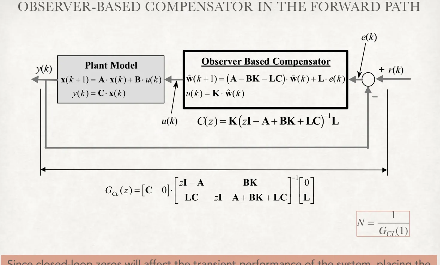
OBSERVER-BASED COMPENSATOR IN THE FORWARD PATH

ME561 WINTER 2012

e(e(kk)) Observer Based Compensator

Observer Based Compensator

++

−−

rr(k(k)) Plant Model

Plant Model y(y(kk))

u(u(k)k)

G z z

CL( ) = ⋅ − z

− + +

L NM O

QP L NM O

QP

−

C I A BK

LC I A BK LC L

0 ¹ 0

x A x B

C x

( ) ( ) ( )

( ) ( )

k k u k

y k k

+ = ⋅ + ⋅

= ⋅

1 ( ) ( ) ( )

( ) ( )

w A BK LC w L

K w

k k e k

u k k

+ = − − ⋅ + ⋅

= ⋅

1

b g

C z ( ) = K I A BK LC L b z − + + g

⁻¹

Figure 8.6 Observer-Based Compensator in the Forward Path P P r r e e d d i i c c t t i i o o n n O O b b s s e e r r v v e e r r - - B B a a s s e e d d C C o o m m p p e e n n s s a a t t o o r r

Although a full order state observer, Eq. (8.22), is used in the previous derivation of the observer- based compensator, there is no reason to restrict yourself to this type of observers. If a full order observer with predication, Eq. (8.24) is used, the overall closed-loop system can be written as

( )

[ ]

( 1) ( )

( 1 1) ( ) ( ) ( )

( ) ( )

( )

k k

k k k k r t

y k k

k k

+ −

⎡ ⎤ ⎡ ⎤ ⎡ ⎤ ⎡ ⎤

= + ⋅ ⋅

⎢ + + ⎥ ⎢ ⎣ − ⎥ ⎦ ⎢ ⎥ ⎢ ⎥ ⎣ ⎦

⎣ ⎦ ⎣ ⎦

⎡ ⎤

= ⎢ ⎥

⎣ ⎦

x A BK BK x B

x 0 I LC A x 0 N

C 0 x x

(8.34)

and the separation principle still applies, i.e. the closed-loop characteristic equation is

( )

( ) ( ) ( )

det z det det 0

z z

z

− − −

⎡ ⎤

= ⎡ − − ⎤ ⋅ ⎡ − − ⎤ =

⎢ − − ⎥ ⎣ ⎦ ⎣ ⎦

⎣ ⎦

I A BK BK

I A BK I A LCA

0 I A LCA

The properties of the closed-loop system described by Eq. (8.34) are analogous to the system described by Eq. (8.30) and are left as an exercise. Note, however, that the observer gain matrix L does not have to be changed when the observer structure is changed. This is a very convenient consequences of the separation principle.

Example 8.9 Observer-Based Compensator Design

A voltage mode DC motor positioning system can be modeled by the following dynamic equations:

J T T T T K i T B T

L di

dt R i K V

M f L M T A f F

A A

A A b IN

, ,

θ ω

ω

= − − = ⋅ = ⋅ +

+ ⋅ + ⋅ =

where

J: Effective inertia at the motor end q ^: Motor angular displacement

T

_M

: Motor torque w : Motor angular velocity

N = 1 G

_CL

(1)

Since closed-loop zeros will affect the transient performance of the system, placing the compensator in the forward path requires careful consideration and the designer should

make sure that the additional zeros will not introduce undesirable transient response.

(36)

P-C OBSERVER-BASED COMPENSATOR P-C Observer-Based Compensator

( k + = ⋅ 1) ( ) k + ⋅ ( ) k

x A x B u ^{u k} ^{( )} ^{= − ⋅} ^{K x} ^ˆ ^{( | )} ^{k k} ^{+ ⋅} ^N ^{r k} ^{( )}