國立臺灣大學社會科學院經濟學系 碩士論文
Department of Economics College of Social Sciences National Taiwan University
Master Thesis
用經濟學實驗研究不同策略性溝通賽局下的 說謊與測謊行為
Cheap Talk Games: Direct and Simplified Replications
謝富文 Fu-Wen Hsieh
指導教授﹕王道一 博士
Advisor: Joseph Tao-Yi Wang, Ph.D.
中華民國 104 年 1 月 January, 2015
摘要
我們重現王道一等人(2010)設計的傳訊賽局實驗,讓一個知道真實狀態的傳訊者 送訊息給(試圖按照真實狀態)做決定的接收者,但兩人之間有利益衝突:傳 訊者有誘因吹噓真實狀態。我們的實驗結果顯示台灣受試者的行為模式與文獻 類似,同樣都傾向「過度溝通」──所傳訊息比均衡預測揭露更多關於真實狀
態的資訊。我們也能根據 level-k 模型把每個受試者分類為不同思考層次的類
型。我們在做完重現實驗之後緊接著另外做只有三種真實狀態的簡化版實驗(並 加上兩種吸引受試者注意力的特異回合)。我們發現簡化版實驗的結果比較接 近理論預測,而且會有更多的受試者被我們歸類成可以想兩層的類型 L2。
關鍵字: 傳訊者-接收者賽局、策略性訊息傳遞、說謊、測謊、實驗室實驗
i
Cheap Talk Games: Direct and Simplified Replications
Fu-Wen Hsieh and Joseph Tao-yi Wang* 30st December, 2014
Abstract
We replicate the experiment designed by Wang, Spezio, and Camerer (2010), in which an informative sender advises an uninformed receiver to take an action (to match the true state), but has incentives to exaggerate. We find similar behavior patterns with Taiwanese subjects. In particular, we also find
“over-communication”—messages reveal more information about the true state than what equilibrium predicts, and classify subjects into various level-k types.
In addition, we conduct a Simplified version of the same experiment with only three states (and two sets of “catch” trials to keep subjects attentive). We find the results are more close to prediction of equilibrium model in this simplified replication, and more senders are classified as L2.
J.E.L. classification codes: C72, C91, D83
Keywords: Sender-Receiver Game, Strategic Information Transmission, Lying, Lie Detection, Laboratory Experiment
*Department of Economics, National Taiwan University, 21 Hsu-Chow Road, Taipei 100, Taiwan. Fu-Wen Hsieh:
[email protected]; Joseph Tao-yi Wang: [email protected]. Shu-Yu Liu, Meng-Chien Su and Ally Wu provided excellent research assistance. We thank comments from Chen-Ying Huang, Pohan Fong, and Jian-Da Zhu.
We thank financial support from the Ministry of Science and Technology of Taiwan (MOST 102-2628-H-002-002-MY4). All remaining errors are our own.
ii
Contents
1. Introduction ... 1
2. The Sender-Receiver Game ... 5
3. Experimental Design and Procedure ... 8
4. Experimental Results ... 10
4.1 Aggregate Results: Final Choice ... 10
4.1.1 Replicate Treatment ... 11
4.1.2 Simplified Treatment ... 15
4.1.3 Individual Choice ... 17
4.2 Correlation, Prediction and Average Payoff ... 17
4.3 Type Classification ... 20
5. Conclusion ... 26
Reference ... 28
Appendix: ... 30
Experimental Instructions ... 38
iii
L IST OF F IGURES
FIGURE 1:PAYOFF TABLE IN SCREEN ... 9
FIGURE 2:SENDER’S EXPECT PAYOFF,REPLICATE TREATMENT ... 14
FIGURE 3:RECEIVER’S EXPECT PAYOFF,REPLICATE TREATMENT ... 14
FIGURE 4:SENDER’S AND RECEIVER’S EXPECT PAYOFF,SIMPLIFIED TREATMENT, BIAS=1 .... 16
FIGURE 5:TYPE CLASSIFICATION OF BOTH,REPLICATE, AND SIMPLIFIED TREATMENT ... 22
iv
List of Tables
TABLE 1-BEHAVIORAL PREDICTIONS OF THE LEVEL-K MODEL (REPLICATE) ... 6
TABLE 2-BEHAVIORAL PREDICTIONS OF THE LEVEL-K MODEL (SIMPLIFIED) ... 7
TABLE 3:PAYOFF TABLES IN EXPERIMENT ILLUSTRATION ... 9
TABLE 4:FINAL CHOICES UNDER BIAS=1,REPLICATE TREATMENT ... 12
TABLE 5:FINAL CHOICES UNDER BIAS=2,REPLICATE TREATMENT ... 12
TABLE 6:FINAL CHOICES UNDER BIAS=1,SIMPLIFIED TREATMENT ... 16
TABLE 7:COMPARISON OF SENDERS’ TYPE, INDIVIDUAL CHOICES ... 17
TABLE 8:INFORMATION TRANSMISSION:CORRELATION BETWEEN STATES,MESSAGES, ACTIONS ... 18
TABLE 9:PROBABILITY OF CORRECT PREDICTIONS, BIAS=1 ... 19
TABLE 10:SUBJECT PREDICTIONS AND ACTIONS OF GIVEN MESSAGE, BIAS 1 ... 19
TABLE 11:AVERAGE PAYOFF OF SENDERS AND RECEIVERS AND PREDICTED IN EQUILIBRIUM 20 TABLE 12:CHANGE OF TYPES BETWEEN REPLICATE AND SIMPLIFIED TREATMENTS ... 22
TABLE 13:ROBUSTNESS CHECK OF TYPE CLASSIFICATION ... 23
TABLE 14:ROBUSTNESS CHECK OF RESAMPLE,REPLICATE TREATMENT,20 PERIODS ... 24
TABLE 15:ROBUSTNESS CHECK OF RESAMPLE,SIMPLIFIED TREATMENT,36 PERIODS ... 25
v
TABLE 16:ROBUSTNESS CHECK OF RESAMPLE,REPLICATE TREATMENT,36 PERIODS ... 25
TABLE 17:ROBUSTNESS CHECK OF RESAMPLE,SIMPLIFIED TREATMENT,20 PERIODS ... 25
TABLE 18:IDENTIFY 3 CASES FOR POTENTIAL FMRI RESEARCH ... 27
vi
1. Introduction
We acquire information from parents, friends, advisers, salespersons, doctors and so on;
however, conflict of interest affects the way we cope with these information. Consumers tend to be skeptical about salespersons introducing their products because they know salespersons have incentives to lie. This is an example of a strategic sender-receiver game where senders have information advantage and their preferences are not aligned with receivers who make decisions.
The amount of information transmitted is affected by how strong the conflicts of interest are between senders and receivers. Similar examples include analysts vs. investors, doctors vs.
patients, candidates vs. interviewers and so on.
Crawford and Sobel (1982) consider a one-dimensional sender-receiver game of strategic information transmission. A Sender who has full information sends a message to a Receiver, and the Receiver takes an action that decides payoffs of both players. Crawford and Sobel (1982) predict that information transmission decreases as the preference difference between Sender and Receiver increases. They also predict no informative equilibrium exists when conflict of interest is sufficiently large. That is, “babbling equilibrium” is the most informative equilibrium.
Experimental economists have used controlled experiments to test theoretical predictions of Crawford and Sobel (1982). In addition, these experiments are conducted in various numbers of states, messages and actions. Gneezy (2005) reports the senders are more likely to lie when loss to receiver decreases or profit to sender increases in a simple sender-receiver game with 2 states
1
x 2 messages x 2 actions. The experiments of Dickhaut et al. (1995) Cai and Wang (2006) and Wang et al. (2010) study the behavior of subjects with different conflict of interest between senders and receivers. Dickhaut et al. (1995) show that as preferences diverge, less information are transmitted in a sender-receiver game with 4 states, 4 actions and messages being single or consecutive sequence of integers from 1 to 4.1 The evidence in Cai and Wang (2006) shows that senders “overcommunicate” and send informative messages to receivers, even though the equilibrium model predicts a “babbling equilibrium”. Cai and Wang (2006) study sender-receiver games with 5 states, 9 actions (5 actions corresponding to each states and 4 intermediate action) and messages being any combination of states.2 Wang et al. (2010) uses eye-tracking to monitor the behavior of senders in sender-receiver games where the numbers of states, messages and actions are all 5. Senders see a state and send one message from {1, 2, 3, 4, 5}, and receivers choose an action from {1, 2, 3, 4, 5}.3
The number of states (and corresponding messages and actions) would influence communication. As the number increases, it is possible for more potential reactions and deception. Hence, the process of information transmission can become more complicated, even though the equilibrium model would predict the same most informative equilibrium.
Sender-receiver games with different parameter space and conditions are extensively studied in the past, but few research compare the results across different state space. We replicate and
1 The messages could be {1}, {2}, {3}, {4}, {1, 2}, {2, 3}, {3, 4}, {1, 2, 3}, {2, 3, 4}, {1, 2, 3, 4}.
2 The states space is {1, 3, 5, 7, 9} and the actions space is {1, 2, 3, 4, 5, 6, 7, 8, 9}. Senders could send messages like {1, 7}, {3, 5} by using or button.
3 The experiments could further extend; for example, allow receivers to costly punish the liars; allow senders to costly keep silence; allow senders to send vague messages; two senders communicate with one receiver and so on [see Sanchez-Pages and Vorsatz (2007, 2009), Serra-Garcia et al. (2011), Vespa and Wilson (2014)].
2
modify the experiment design of Wang et al. (2010). Our experiment has two parts, one is the Replicate Treatment with 5 state space as in Wang et al. (2010), and the other is the Simplified Treatment with only 3 state space. The Simplified Treatment uses the similar experimental procedures, but has a smaller state space and fewer biases.4 We focus on the comparison of senders’ behavior in the two Treatments.
We compare the results of the two Treatments. The aggregate and comparative static results show that subject behavior is closer to equilibrium prediction in the Simplified Treatment than the Replicate Treatment. The equilibrium model fails to explain the abundant amount of low-type (L0 and L1) messages, while the level-k model can.
Stahl and Wilson (1994), Nagel (1995), and Camerer et al. (2004) pioneered steps-of-reasoning models of bounded rationality. In the level-k model of Stahl and Wilson (1994) and Nagel (1995), subjects incorrectly believe their opponents have a specific level of bounded rationality, and play best response to this (naïve) belief. In contrast, the cognitive hierarchy model of Camerer et al. (2004) assume subjects have correct but truncated beliefs about others since they cannot image the reasoning of higher types than themselves due to limited cognition.
Crawford (2003) analyses sender-receiver game with level-k model, and sets the L0 sender with truth-telling rather than random-choosing. Costa-Gomes and Crawford (2006) reports that level-k model explains the predictable component of systematic deviations from equilibrium well.
Cai and Wang (2006) uses level-k model to explain their results. Kawagoe (2009) reports that the
4 As the state space decrease, the required “sufficient large” bias which leads to babbling equilibrium will decrease.
3
level-k analysis explains their results better than other theories. Our results support the level-k analysis.
Using maximum likelihood estimations, we classified senders into L0 to L2 types and evaluate type classification stability by resampling senders’ choices. 12-14% of senders are classified as L0 type in both Treatments. The proportion of L1 senders decrease from 39% to 25% when the state space decreases from 5 to 3. In contrast, more senders are classified as L2 type in the Simplified Treatment. Resampling of senders’ choices shows that L2 senders are more stable in the Simplified Treatment. These results are consistent with the level-k model (but not cognitive hierarchy) since the more complicated Replicate Treatment should induce senders to think their opponents have lower levels of reasoning.
The remainder of this paper is organized as follows. We formulate some theoretical predictions and propose a set of hypotheses in section 2. Section 3 explains the design of our experiments. Section 4 analyzes our experimental results and section 5 concludes.
4
2. The Sender-Receiver Game
This paper follows the experiment designed by Wang, Spezio, and Camerer (2010); there are two parts: one is almost the same with the former paper, which is called the Replicate treatment; the other is a simplified version which might have an extended functional magnetic resonance imaging (fMRI) research, which is called the Simplified treatment.
In the first part of experiment, the Replication design, the sender is informed about the true state s at the beginning of every period, which is unknown to receiver and drawn from state space S = {1, 2, 3, 4, 5} with the same probability. Meanwhile, the sender is also informed about bias b, which is known to both sender and receiver. Bias could be either 0, 1, or 2 (realized number and public information, so we do not inform subjects about the probability distribution). Then sender sends a message to receiver from message space M = {1, 2, 3, 4, 5}.
After that the receiver chooses an action a from action space A = {1, 2, 3, 4, 5}. Payoffs of Receiver are decided by functions uR = 110 − 20 |s − a|1.4; Payoffs of Sender are decided by
functions uS = 110 − 20 |s + b − a|1.4. Sender will obtain best payoffs when receiver choose
action equal to state plus bias. However, receiver wants to choose action equal to state.
In the second part of experiment, the state, message, and action space change from {1, 2, 3, 4, 5} to {1, 2, 3}, the state is drawn with the same probability. The bias is shifted to {-1, 0, 1}, b = -1 has low rates of occurrence.
5
Wang, Spezio, and Camerer (2010) derive the level-k model for the sender-receiver game, begin with L0 senders send message truthfully and L0 receivers accept the message by taking the action equal to it. Then L1 senders best respond to L0 receivers, L1 receivers best respond to L1 senders and so on (see Table 1 and Table 2).
Table 1-Behavioral Predictions of the Level-k Model (Replicate)
Sender message (condition on state) Receiver action (condition on message)
State 1 2 3 4 5 Message 1 2 3 4 5
b=0
L0/EQ sender 1 2 3 4 5 L0/EQ receiver 1 2 3 4 5
b=1
L0 sender 1 2 3 4 5 L0 receiver 1 2 3 4 5 L1 sender 2 3 4 5 5 L1 receiver 1 1 2 3 4 L2 sender 3 4 5 5 5 L2 receiver 1 1 1 2 4 EQ/L3 sender 4 5 5 5 5 EQ/L3 receiver 1 1 1 1 4 SOPH sender 3 4 5 5 5 SOPH receiver 1 1 2 3 4
b=2
L0 sender 1 2 3 4 5 L0 receiver 1 2 3 4 5 L1 sender 3 4 5 5 5 L1 receiver 1 1 1 2 4 L2 sender 4 5 5 5 5 L2 receiver 1 1 1 1 4 EQ/L3 sender 5 5 5 5 5 EQ/L3 receiver 1 1 1 1 3 SOPH sender 5 5 5 5 5 SOPH receiver 2 2 2 3 4
6
Table 2-Behavioral Predictions of the Level-k Model (Simplified)
Sender message (condition on state) Receiver action (condition on message)
State 1 2 3 Message 1 2 3
b=0
L0/EQ sender 1 2 3 L0/EQ receiver 1 2 3 b=1
L0 sender 1 2 3 L0 receiver 1 2 3
L1 sender 2 3 3 L1 receiver 1 1 2
EQ/L2 sender 3 3 3 EQ/L2 receiver 1 1 2
SOPH sender 3 3 3 SOPH receiver 1 2 2
b=-1
L0 sender 1 2 3 L0 receiver 1 2 3
L1 sender 1 1 2 L1 receiver 2 3 3
EQ/L2 sender 1 1 1 EQ/L2 receiver 2 3 3
When the type gets higher, there will be more difficult to tell a type (Ln) from a higher type (L(n+1)) of senders. In Replicate Treatment, the difference between L0 and L1 senders will occur in 8 cases (b = 1, 2 with s = 1, 2, 3, 4); similarly, the difference between L1 and L2 senders occur in 5 cases (b = 1, s = 1, 2, 3 and b = 2, s = 1, 2). And L2 could only be tell from L3 type senders in 3 cases; consequently, more periods are needed if we want to identify a pair of types which have small difference.
7
3. Experimental Design and Procedure
We conducted a total of 8 sessions at the Taiwan Social Sciences Experiment Laboratory (TASSEL) in National Taiwan University (NTU), consisting of 118 subjects with 10 to 20 subjects in one experiment. We made announcement on online forums (ptt.cc, the largest Bulletin Board System in Taiwan) and via email sent to the TASSEL subjects pool. Subjects are NTU undergraduate or graduate students, which voluntarily signed up on TASSEL’s online recruiting website. They were paired randomly to play 20 periods in part 1 and, 405 periods in part 2. The exchange rate is 6 Experimental Standard Currency (ESC) for NT$1. Subjects earned NT$623 to NT$1001 (including a NT$100 show up fee), with an average of NT$ 860.8 (approximately US$ 28.7). Experiment typically lasted for 2.5 hours to 3 hours.
All experiments were conducted in Chinese using Z-Tree (Zurich Toolbox for Readymade Economic Experiments, developed by Fischbacher, 2007). Subjects were informed the game instruction and then assigned to the role of sender or receiver randomly.
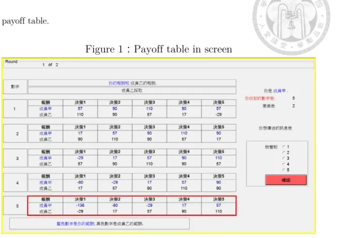
In Part 1, the Replication design, there are 3 exercise periods and 20 paid periods. Subjects were assigned as the same role in all 23 periods. States are drawn with equal probabilities, biases 0, 1, 2 are drawn with probabilities 0.2, 0.4 and 0.4, respectively. Subjects are informed the payoffs both payoff tables on the screen and experimental instructions (see Figure 1 and Table 3).
Since we did not eye-track our subjects, we did not follow Wang, Spezio, and Camerer (2010) to
5 In experiment 3, part 2 only has 35 periods because z-tree crashed.
8
add a small random number to the payoffs to make it an uncertain number, so subjects will look at the payoff table.
Figure 1:Payoff table in screen
Table 3:Payoff tables in Experiment illustration
State-Action 0
Sender Payoff 110 90 57 17 -29
State+Bias-Action 0
Receiver Payoff 110 90 57 17 -29 -80 -136
9
In Part 2, the Simplified design, there are 36 periods with bias = 0 or 1. Subjects played the same role as in Part 1. States are drawn with equal probabilities, biases 0, 1 are drawn with probabilities 0.25 and 0.75, respectively. In addition, there are 4 “catch” trials added randomly to attracting attention of the subject (for potential future fMRI research). Two event are joined in the second game: change role and negative bias, subject is assigned to sender or receiver throughout whole experiment except certain periods in the Simplified design; subjects are assigned to another role or the bias are allocated to -1 in two periods, respectively. Two event are not allowed to occur at the same time. The sender is requested to predict the action of receiver after sending message, they will earn extra 3 ESC if the prediction is equal to action.
Level-k model and decision-making pattern of senders are combined for type-classification, we use a quantal response-like logit error structure to estimate the type of senders.
4. Experimental Results
4.1 Aggregate Results: Final Choice
We report results after dropping the two type of catch trials in the Simplified treatment.
These events are designed to attract subject attention. Results including these trials (Tables A22-A27 in the Appendix) are similar to results without catch trials.
10
Regardless of treatment, senders tell the truth and receivers follow their advice when bias is 0. In fact, only 8 out of 245 periods (4 of 245 periods) do we see sender not sending message equal to the true state (receiver not taking action equal to the message) in the Replication treatment. Meanwhile, none of the senders send messages different from the true state and only 2 out of 542 periods do the receiver not take action equal to message when bias is 0 in the Simplified treatment.
4.1.1 Replicate Treatment
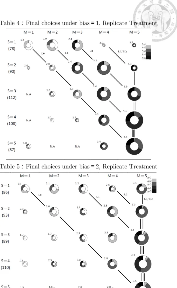
Table 4 and 5 report results of b = 1 and 2 in the Replicate treatment. The size of the doughnut charts in Table 4 and 5 are scaled by the frequency of occurrence for senders sending message conditional on a given state. The fractions in each doughnut chart represents actions taken by receivers for each message and state, the darker the color, the higher the action. The number near each doughnut chart is the average action taken by the receivers. Note that the receiver only knows the message, not the true state, so the average action for different states given a certain message are very similar. The average action increases as the message becomes larger.
11
Table 4:Final choices under bias=1, Replicate Treatment
Table 5:Final choices under bias=2, Replicate Treatment
12
As the level-k model predicts, charts locate above the diagonal are larger than those below.
When b = 1, charts are largest when they are 1 or 2 (L1 or L2) steps above the diagonal (L0).
Note that since the matrix is bounded, senders are predicted to all send message 5 when the state is 5. When b = 2, messages that are two steps above the diagonal (L0) indicate L1, and more states (3 to 5) are predicted to exhibit message 5. Messages are now closer to the babbling equilibrium (all sending 5) than b = 1. This is partly predicted by the level-k model, but the frequency of L1 choices seems to be lower. These aggregate results are consistent with Wang, Spezio, and Camerer (2010).
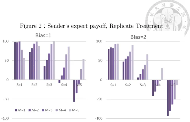
Both senders and receivers do well in experiment. Figure 2 reports sender’s E(π) for sending different messages, and Figure 3 shows receivers’ E(π) for taking different actions. For most states, senders usually choose the message that yield the highest or second-highest payoff.
Two exceptions occur when s=1, 2 for b=2; in that case, the difference between each
message’s expect payoffs are small. For most messages, receivers normally take the action that yield the highest or second-highest payoff. Since subjects rarely send message 5 when the true state is 1 or 2, this increases the likelihood of having higher states when seeing a message of 5, which induces receivers to choose higher actions. When the message is 5, the average action taken by receivers is 3.4 in our experiment, very close to that of Wang, Spezio, and Camerer (2010), both higher than what babbling equilibrium predicts.
13
Figure 2:Sender’s expect payoff, Replicate Treatment
Figure 3:Receiver’s expect payoff, Replicate Treatment
14
4.1.2 Simplified Treatment
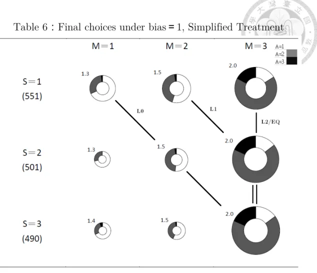
In Table 6, the size of doughnut charts are re-scaled because the largest donut chart increases from 70 to 409, and the message space is reduced from 5 to 3. The results are close to the babbling equilibrium (all messages are 3), and similar to that of b = 2 in the Replicate Treatment. Senders sometimes do not send the equilibrium message of 3 when state is 1, but split between 1 and 2 instead. This reveals some information regarding the true state.
Seeing message is 3, receivers take average action of 2, which is the same as the babbling equilibrium prediction.
Figure 4 shows that senders earn the most when sending messages equal to 3. However, sending other messages still yields payoffs close to the optimal when state is 1. So, the cost of sending these messages is low, which explains the abundance of such messages. Seeing that message is 3, receivers earn the most by taking action equal to 2.
15
Table 6:Final choices under bias=1, Simplified Treatment
Figure 4:Sender’s and Receiver’s expect payoff, Simplified Treatment, bias=1
16
4.1.3 Individual Choice
In the aggregate data, higher proportion of L2 or higher messages are sent in the
Simplified Treatment, so we examine individual data of each sender. We exclude the bias and state combinations which messages of L1 and L2 level coincide. We then classify a sender as a High (L2 or above) or Low (L1 or below) type if the sender sends Low or High level messages more than 3/4 of the time. Otherwise, sender is classified as a mixed type. We compare each sender’s type in the Replicate Treatment and Simplified Treatment.
The results are shown in Table 7. More than half senders do not change their types across treatments. 15 senders are Low types in both Treatments, 5 are mixed types, and 13 are High types. 20 out of 59 senders increase their types in the Simplified Treatment. In contrast, only 6 senders decrease their types in the Simplified Treatment.
Table 7:Comparison of senders’ type, individual choices
Sim Low Sim Mix Sim High
Rep Low 15 6 5
Rep Mix 4 5 9
Rep High 1 1 13
4.2 Correlation, Prediction and Average Payoff
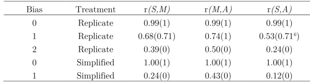
Table 8 shows the Comparative Static Results of Correlation between States, Messages, and Actions. The predictions of correlation by equilibrium model is in parenthesis. The results are the same with that reported by Wang, Spezio, and Camerer (2010) and prediction made by
17
Crawford and Sobel (1982): The correlations decrease when bias increase, even though the empirical correlations do not exactly match theory. This is because subjects’ behavior patterns seem to follow the level-k model instead of equilibrium. This results in overcommunication when b is large, adherence to the truth-telling equilibrium when b=0, and heterogeneous choices when b=1 in the Replicate Treatment. Individual subjects may also exhibit noisy
behavior which lowers aggregate correlation.
Equilibrium model predicts babbling equilibrium when bias is 2, i.e. senders always send messages equal to 5 and receivers take actions only by their prior belief of the true states.
Therefore, correlation between states, messages, and actions will be 0 in this case. Instead, the correlations of our data do not close to 0, which are called “over-communication” in Cai and Wang (2006). In the Simplified Treatment, the correlations of actual data and prediction given bias is 0 (1) are similar to those of bias equal to 0 (2) in the Replicate Treatment.
Table 8 : Information Transmission:Correlation between States, Messages, Actions
Bias Treatment r(S,M) r(M,A) r(S,A)
0 Replicate 0.99(1) 0.99(1) 0.99(1)
1 Replicate 0.68(0.71) 0.74(1) 0.53(0.716)
2 Replicate 0.39(0) 0.50(0) 0.24(0)
0 Simplified 1.00(1) 1.00(1) 1.00(1)
1 Simplified 0.24(0) 0.43(0) 0.12(0)
6 The correlation between States and Actions would be 0.71, predicted by the level-k model in equilibrium (EQ), Wang, Spezio, and Camerer (2010) might misreport it as 0.65.
18
The probability of senders’ prediction (about receiver’s choice) equal to the action taken by receivers is 53% (see Table 9). And the aggregate data shows that prediction of senders and action taken by receivers are different (see Table 10). The rate of correct predictions increases as the message increases. The number in parenthesis presents the total amount of each message.
And the lighter the color, the smaller the action (prediction). The number near doughnut charts is the average action or prediction.
Table 9:Probability of correct Predictions, bias=1
P( =A)M=1,2,3 P( =A)M=1 P( =A)M=2 P( =A)M=3
0.53 0.37 0.41 0.59
Table 10: Subject Predictions and Actions of given Message, bias 1
A Message 1
(179)
Message 2 (258)
Message 3 (1105)
19
Table 11:Average payoff of Senders and Receivers and predicted in equilibrium
Replicate Treatment
Bias uS Predicted uS uR Predicted uR
0 109.10(4) 110(0) 109.10(4) 110(0)
1 81.48(30) 87.40(17) 88.65(23) 91.40(19) 2 40.58(55) 49.00(50) 78.27(31) 80.80(21)
Simplified Treatment
Bias uS Predicted uS uR Predicted uR
0 99.89(2) 100(0) 99.89(2) 100(0)
1 55.77(39) 63.67(33) 75.88(24) 80.80(14)
All the average payoffs are lower than predicted in equilibrium but standard deviation are larger than prediction (shown in Table 11). The number in parenthesis is the standard deviation of each payoff. This shows a potential Pareto improvement for the subject. The difference between average and prediction payoff of senders is larger than receivers. It could result in concave payoff function and untouchable ideal point of senders (in some cases that state plus bias is larger than 5). Therefore, the cost of mistake taken by senders are larger than receivers.
We have try to split the data into first and last part for examining the learning effect.
Table A30-A33 in Appendix show that the learning effect is quiet small. Sometimes the correlation converge to the prediction of equilibrium model but sometimes not.
4.3 Type Classification
We use data from each experiment to estimate the type of senders, by assuming that
sender have a certain level-k type and choose the message with probability ,
20
is the expect payoff of sending message = m given state=s. Maximum Likelihood Estimations are made by using this logit error structure.
We classify the type of senders as L0 to L2 in Both Treatment (data include Both, Replicate, or Simplified). Why we do not classify L3 and SOPH types? First, the SOPH type is exactly the same with L2 in Simplified Treatment. The results are shown in Table 1 and 2.
Second, in the Replicate Treatment, the SOPH type acts like L2 when bias is 1, but acts like L3 when bias is 2. Hence, the difference between L2 and SOPH type are only found in one case (b
= 2, s = 1). Likewise, there are only 2 cases that tell L3 from SOPH (b = 1, s = 1, 2), while L2 and L3 differ in only 3 cases.7 One case will occur at expected 1.6 periods8 in Replicate Treatment. Wang et al. (2010) has 45 periods but we have only 20 periods in our experiment.
It would have difficulty to separate L2, L3, and SOPH type apart.
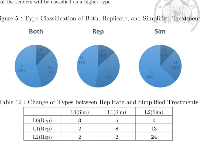
Figure 5 shows the main results of type classification.9 In the Simplified Treatment, 12%
of senders are classified as L0 type; 25% of senders are classified as L1 type; 63% of senders are classified as L2 type. In the Replicated Treatment, the proportion of L0 type hardly changes, while proportion of L1 type increases from 25% to 39%.
Table 12 compares the types classified with data from Replicate or Simplified Treatment.
Senders who are classified as L2 type in the Replicate Treatment usually are also classified as L2 type in the Simplified Treatment. However, if sender are not classified as L2, more than
7 The 3 cases are the 1 case that differs L2 and SOPH and the 2 cases that differs L3 and SOPH.
8 Bias 1 and 2 have 0.4 probability to occur and States are drawn uniformly. That is 20*0.4*0.2=1.6 periods on average.
9 Baseline uses logit error structure and data without bias=0.
21
half of the senders will be classified as a higher type.
Figure 5:Type Classification of Both, Replicate, and Simplified Treatment
Table 12:Change of Types between Replicate and Simplified Treatments
L0(Sim) L1(Sim) L2(Sim)
L0(Rep) 3 5 0
L1(Rep) 2 8 13
L2(Rep) 2 2 24
We also conduct some robustness checks. Table 13 shows the proportion that senders are classified as the same type across 2 or 3 specifications. To begin, we classify subjects as L0 to L3 in the Replicate Treatment, the result is 7 (12%) senders who are classified as L2 are now classified as L3. Next, we compare the results of both the Replicate and the Simplified Treatment, the Replicate Treatment, and the Simplified Treatment. In that case, 78% of senders are identified as the same type through 3 kinds of data. Then we compare logit and spike-logit error structure in Replicate Treatment. Only 10% of senders are classified as other types. Finally, we compare the results of data with or without b = 0 in 3 data pools. Just a small number of senders will be identified as different type.
22
Table 13:Robustness Check of Type Classification
Comparison between difference condition
Identified as the same type Both vs. Rep vs. Sim 78%
Rep_logit vs. spikelogit 90%
Both_notb0 vs. withb0 97%
Rep_notb0 vs. withb0 93%
Sim_notb0 vs. withb0 100%
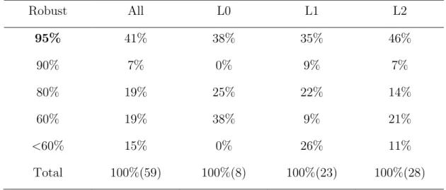
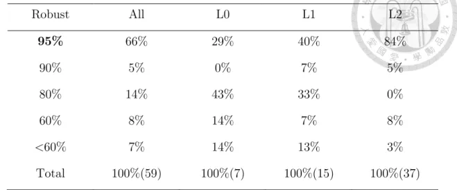
To examine the robustness of type classification, we resample our data 1000 times with replacement. In the Replicate Treatment, we draw 20 periods. In the Simplified Treatment, we draw 36 periods10. In addition, we use the same method which is described earlier to classify sender types. We report the times which are classified as the same type of original data.
The results are shown in Table 14-15.11 The total number of senders are in the
parentheses. In the Replicate Treatment, about 40% of L0 to L2 senders are classified as the same type more than 95% of the time. However, 84% of L2 senders are classified as L2 type more than 95% of the time in the Simplified Treatment. In brief, more senders are classified as L2 sender and the results is more stable in the Simplified Treatment.
One possibility is that there are more periods in the Simplified Treatment than Replicate Treatment. To address this, we resample the two treatment both for 20 and 36 periods. The results are shown in Table 16-17. Comparing Table 15 with Table 16, 30% more of the L2 senders in the Simplified Treatment are 95% stable than in the Replicate Treatment. Similarly,
10 We exclude the periods where bias is -1 or roles are reversed in the Simplified Treatment. In session 3, even though we only have data of 31 periods in the Simplified Treatment because z-tree crashed. We also draw 36 periods.
11 More details are in Appendix table 1-4.
23
in the comparison of Table 14 and Table 17, the Simplified Treatment has 24% more stable L2 senders than Replicate Treatment. In contrast, comparing the same treatment but different number of rounds, the 36-rounds resampling has only 8-14% more robust L2 senders than the 20-rounds case. Therefore, the numbers of periods explain less than half of the effect.
In models of bounded rationality, the level of subject is decided by two factors: the maximum level one could infer, as considered in Camerer et al. (2004), and one’s belief of the opponents’ level, as in Costa-Gomes and Crawford (2006). In most applications, one cannot easily separate these two factors. In our data, having the same maximum level one can infer cannot explain why some senders are classified as low levels in the Replicate Treatment but as high levels in the Simplified Treatment. In contrast, beliefs about opponent levels are more likely to vary across environments. Since the Replicate Treatment is relatively complicated, some senders might think their opponents have lower level of thinking and send low level messages.
Table 14:Robustness check of resample, Replicate Treatment, 20 periods
Robust All L0 L1 L2
95% 41% 38% 35% 46%
90% 7% 0% 9% 7%
80% 19% 25% 22% 14%
60% 19% 38% 9% 21%
<60% 15% 0% 26% 11%
Total 100%(59) 100%(8) 100%(23) 100%(28)
24
Table 15:Robustness check of resample, Simplified Treatment, 36 periods
Robust All L0 L1 L2
95% 66% 29% 40% 84%
90% 5% 0% 7% 5%
80% 14% 43% 33% 0%
60% 8% 14% 7% 8%
<60% 7% 14% 13% 3%
Total 100%(59) 100%(7) 100%(15) 100%(37)
Table 16:Robustness check of resample, Replicate Treatment, 36 periods
Robust All L0 L1 L2
95% 51% 50% 48% 54%
90% 8% 0% 9% 11%
80% 14% 38% 9% 11%
60% 17% 13% 13% 21%
<60% 10% 0% 22% 4%
Total 100%(59) 100%(8) 100%(23) 100%(28)
Table 17:Robustness check of resample, Simplified Treatment, 20 periods
Robust All L0 L1 L2
95% 51% 29% 13% 70%
90% 14% 0% 27% 11%
80% 10% 29% 7% 8%
60% 17% 14% 40% 8%
<60% 8% 29% 13% 3%
Total 100%(59) 100%(7) 100%(15) 100%(37)
25
5. Conclusion
We replicate the experiment of Wang et al. (2010). Furthermore, we conduct a simplified version and compare the results of both Treatments. The results of direct Replication are similar to that Wang et al. (2010). The behavior of subjects in the Simplified Treatment are closer to babbling equilibrium than in b = 2 of Replicate Treatment. The type of senders are classified as only L0 to L2. In addition, more senders are classified as L2 in the Simplified Treatment than in the Replicate Treatment. In the same way, more senders increase their proportion of choosing High (L2 or above) types in the Simplified Treatment than decrease, likely because it simpler game.
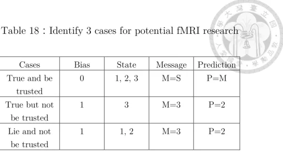
We could classified the choices of a L1 or L2 type sender into 3 cases in Simplified Treatment (see Table 14). First, when b = 0, the sender will tell the truth and will be trusted. Then, when b = 1 and s = 1 or 2, the sender usually tell a lie and will not be trusted. Finally, when b = 1 and e = 3, the sender will tell the truth but will not be trusted. Hope we can find some difference of brain activities in the potential fMRI research.12
12 In the paper-based post experimental questionnaire, we asked subjects, “Could you finish the tasks in the Simplified Treatment in 6 seconds? If not in the beginning, how many rounds of practice do you need to finish it in 6 seconds?”
78% of senders said they could finish it on time, or require at most 7 rounds of practice. The remaining 22% reported that they need 10 or more rounds before they can finish it on time.
26
Table 18:Identify 3 cases for potential fMRI research
Cases Bias State Message Prediction True and be
trusted
0 1, 2, 3 M=S P=M
True but not be trusted
1 3 M=3 P=2
Lie and not be trusted
1 1, 2 M=3 P=2
27
Reference
Cai, Hongbin and Joseph Tao-yi Wang. 2006. “Overcommunication in Strategic Information Transmission Games” Games and Economic Behavior, 56(1), 7-36.
Camerer, Colin F., Teck-Hua Ho, and Juin-Kuan Chong. 2004. “A Cognitive Hierarchy Model of Games.” Quarterly Journal of Economics, 119(3): 861–98.
Costa-Gomes, Miguel A. and Vincent P. Crawford. 2006. “Cognition and Behavior in Two-Person Guessing Games: An ExperimentaSl tudy.” The American Economic Review, 96(5): 1737-1768
Crawford, Vincent P. 2003. “Lying for Strategic Advantage: Rational and Boundedly Rational Misrepresentation of Intentions.” American Economic Review, 93(1): 133–49.
Crawford, Vincent P. and Joel Sobel. 1982. “Strategic Information Transmission”
Econometrica, 50(6): 1431-1451.
Dickhaut, John W. Kevin A. McCabe, and Arijit Mukherji. 1995. “An experimental study of strategic information transmission” Economic Theory, 6(6): 389-403.
Gneezy, Uri. 2005. “Deception: The Role of Consequences.” American Economic Review, 95(1): 384–94.
Kawagoe, Toshiji and Hirokazu Takizawa. 2009. “Equilibrium refinement vs. level-k
28
analysis: An experimental study of cheap-talk games with private information.” Games and Economic Behavior, 66(1): 238-255.
Nagel Rosemarie. 1995. “Unraveling in Guessing Games: An experimental study.” The American Economic Review, 85(5): 1313-1326
Serra-Garcia Marta, Eric van Damme and Jan Potters. 2011. “Hiding an inconvenient truth: Lies and Vagueness.” Games and Economic Behavior, 73(1): 244-261.
Sanchez-Pages, Santiago, and Marc Vorsatz. 2007. “An Experimental Study of Truth-Telling in a Sender-Receiver Game.” Games and Economic Behavior, 61(1): 86-112
Sanchez-Pages, Santiago, and Marc Vorsatz. 2009. “Enjoy the silence: an experiment on truth-telling.” Experimental Economics. 12(2): 220-241
Stahl Dale O. and Paul W. Wilson. 1995. “On players’ models of other players: Theory and experimental evidence.” Games and Economic Behavior, 10: 218-254
Vespa Emanuel and Alistair J. Wilson. 2014. “Communication with Multiple Senders: An experiment.” Working paper.
Wang, Joseph Tao-yi, Michael Spezio and Colin F. Camerer. 2010. “Pinocchio's Pupil:
Using Eyetracking and Pupil Dilation To Understand Truth Telling and Deception in Sender-Receiver Games” American Economic Review, 100(3): 984-1007.
29
Appendix:
Table A1: The number of total trials, given on bias, Replicate
Bias 0 1 2
Frequency 245 475 460
Table A2: Bias=0, Sender matrix, Replicate
Message 1 Message 2 Message 3 Message 4 Message 5 Total
State 1 58 1 0 0 0 59
State 2 1 44 3 0 0 48
State 3 0 1 51 0 0 52
State 4 0 0 1 38 1 40
State 5 0 0 0 0 46 46
Total 59 46 55 38 47 245
Table A3: Bias=1, Sender matrix, Replicate
Message 1 Message 2 Message 3 Message 4 Message 5 Total
State 1 19 29 27 1 2 78
State 2 1 7 30 44 8 90
State 3 0 6 16 46 44 112
State 4 0 2 2 27 77 108
State 5 4 0 0 11 72 87
Total 24 44 75 129 203 475
Table A4: Bias=2, Sender matrix, Replicate
Message 1 Message 2 Message 3 Message 4 Message 5 Total
State 1 16 19 19 8 24 86
State 2 3 19 10 26 35 93
State 3 3 7 12 19 48 89
State 4 5 6 8 21 70 110
State 5 2 4 3 4 69 82
Total 29 55 52 78 246 460
30
Table A5: Bias=0, Receiver matrix, Replicate
Action 1 Action 2 Action 3 Action 4 Action 5 Total
Message 1 57 2 0 0 0 59
Message 2 0 46 0 0 0 46
Message 3 1 0 54 0 0 55
Message 4 0 0 1 37 0 38
Message 5 0 0 0 0 47 47
Total 58 48 55 37 47 245
Table A6: Bias=1, Receiver matrix, Replicate
Action 1 Action 2 Action 3 Action 4 Action 5 Total
Message 1 14 9 1 0 0 24
Message 2 16 18 8 2 0 44
Message 3 5 42 22 6 0 75
Message 4 0 15 66 42 6 129
Message 5 0 2 50 102 49 203
Total 35 86 147 152 55 475
Table A7: Bias=2, Receiver matrix, Replicate
Action 1 Action 2 Action 3 Action 4 Action 5 Total
Message 1 13 9 7 0 0 29
Message 2 17 23 12 3 0 55
Message 3 19 7 17 5 4 52
Message 4 6 35 23 12 2 78
Message 5 12 15 117 74 28 246
Total 67 89 176 94 34 460
Table A8: Bias=1, Expect Payoff of Sender, Replicate
Message 1 Message 2 Message 3 Message 4 Message 5
State 1 98 97 99 78 56
State 2 72 82 94 99 87
State 3 35 51 68 93 100
State 4 -8 11 32 66 86
State 5 -57 -35 -12 28 54
31
Table A9: Bias=2, Expect Payoff of Sender, Replicate
Message 1 Message 2 Message 3 Message 4 Message 5
State 1 80 84 82 93 94
State 2 47 55 61 73 90
State 3 6 15 27 39 66
State 4 -41 -30 -15 -3 30
State 5 -93 -81 -64 -51 -14
Table A10: Bias=1, Expect Payoff of Receiver, Replicate
Action 1 Action 2 Action 3 Action 4 Action 5
Message 1 86 79 58 31 -4
Message 2 95 92 71 38 -5
Message 3 88 97 82 51 11
Message 4 53 84 94 82 54
Message 5 13 52 82 96 86
Table A11: Bias=2, Expect Payoff of Receiver, Replicate
Action 1 Action 2 Action 3 Action 4 Action 5
Message 1 77 81 72 50 15
Message 2 76 88 79 56 21
Message 3 72 85 81 60 26
Message 4 58 84 90 77 46
Message 5 31 63 81 84 67
Table A12: The number of total trials without exchange role, given on bias, Simplified
Bias 0 1 -1
Frequency 542 1542 118
Table A13: Bias=-1, Sender matrix, Simplified
Message 1 Message 2 Message 3 Total
State 1 27 3 1 31
State 2 30 7 4 41
State 3 25 13 8 46
Total 82 23 13 118
32
Table A14: Bias=0, Sender matrix, Simplified
Message 1 Message 2 Message 3 Total
State 1 178 0 0 178
State 2 0 181 0 181
State 3 0 0 183 183
Total 178 181 183 542
Table A15: Bias=1, Sender matrix and reversed matrix of bias=-1, Simplified Message 1 Message 2 Message 3 Total
State 1 107 133 311 551
State 2 35 81 385 501
State 3 37 44 409 490
Total 179 258 1105 1542
Reversed matrix bias = -1
Message 1 Message 2 Message 3
State 1 1 3 27
State 2 4 7 30
State 3 8 13 25
Table A16: Bias=-1, Prediction matrix, Simplified
Prediction 1 Prediction 2 Prediction 3 Total
Message 1 33 44 5 82
Message 2 6 13 4 23
Message 3 1 6 6 13
Total 40 63 15 118
Table A17: Bias=0, Prediction matrix, Simplified
Prediction 1 Prediction 2 Prediction 3 Total
Message 1 177 0 1 178
Message 2 0 181 0 181
Message 3 0 0 183 183
Total 177 181 184 542
33
Table A18: Bias=1, Prediction matrix and reversed matrix of bias=-1, Simplified Prediction 1 Prediction 2 Prediction 3 Total
Message 1 58 98 23 179
Message 2 96 121 41 258
Message 3 56 881 168 1105
Total 210 1100 232 1542
Reverse bias = -1
Prediction 1 Prediction 2 Prediction 3
Message 1 6 6 1
Message 2 4 13 6
Message 3 6 6 1
Table A19: Bias=-1, Receiver matrix, Simplified
Action 1 Action 2 Action 3 Total
Message 1 22 56 4 82
Message 2 1 8 14 23
Message 3 0 4 9 13
Total 23 68 27 118
Table A20: Bias=0, Receiver matrix, Simplified
Action 1 Action 2 Action 3 Total
Message 1 177 1 0 178
Message 2 0 180 1 181
Message 3 0 0 183 183
Total 177 181 184 542
Table A21: Bias=1, Receiver matrix and reserved matrix of bias=-1, Simplified Action 1 Action 2 Action 3 Total
Message 1 123 52 4 179
Message 2 140 112 6 258
Message 3 167 739 199 1105
Total 430 903 209 1542
Reverse bias = -1
Action 1 Action 2 Action 3
Message 1 9 4 0
Message 2 14 8 1
Message 3 4 56 22
34
Table A22:Sender Matrix, Robustness Check, bias=0 Without Catch Trials (Baseline) All Data
M=1 M=2 M=3 M=1 M=2 M=3
S=1 178 0 0 179 0 0
S=2 0 181 0 0 182 0
S=3 0 0 183 0 0 187
Table A23:Sender Matrix, Robustness Check, bias=1 Without Catch Trials (Baseline) All Data
M=1 M=2 M=3 M=1 M=2 M=3
S=1 107 133 311 121 145 348
S=2 35 81 385 42 97 434
S=3 37 44 409 49 62 450
Table A24:Receiver Matrix, Robustness Check, bias=0 Without Catch Trials (Baseline) All Data
A=1 A=2 A=3 A=1 A=2 A=3
M=1 177 1 0 188 1 0
M=2 0 180 1 0 186 1
M=3 0 0 183 0 0 196
Table A25:Receiver Matrix, Robustness Check, bias=1 Without Catch Trials (Baseline) All Data
A=1 A=2 A=3 A=1 A=2 A=3
M=1 123 52 4 143 64 5
M=2 140 112 6 167 130 7
M=3 167 739 199 180 818 234
Table A26:Prediction Matrix, Robustness Check, bias=0 Without Catch Trials (Baseline) All Data
=1 =2 =3 =1 =2 =3
M=1 177 0 1 188 0 1
M=2 0 181 0 0 187 0
M=3 0 0 183 0 0 196
35
Table A27:Prediction Matrix, Robustness Check, bias=1 Without Catch Trials (Baseline) All Data
=1 =2 =3 =1 =2 =3
M=1 58 98 23 72 116 24
M=2 96 121 41 102 151 51
M=3 56 881 168 62 920 181
Table A28: Bias=1, Expect Payoff of Sender, Simplified
Message 1 Message 2 Message 3
State 1 79 83 90
State 2 37 44 68
State 3 -20 -11 21
Table A29: Bias=1, Expect Payoff of Receiver, Simplified
Action 1 Action 2 Action 3
Message 1 78 76 47
Message 2 77 79 50
Message 3 60 80 67
Table A30:Learning Results: Correlation in Replicate Treatment Rounds Bias CorrSM CorrMA CorrSA
1-10
0 0.984 0.998 0.982
11-20 0.998 0.988 0.994
1-10
1 0.644 0.761 0.521
11-20 0.720 0.714 0.542
1-10
2 0.381 0.488 0.192
11-20 0.404 0.524 0.290
Table A31:Learning Results: Payoffs in Replicate Treatment
Rounds Bias u_S (std) u_R (std)
1-10
0 108.67 5.01 108.67 5.01
11-20 109.52 3.07 109.52 3.07
1-10
1 81.07 29.30 89.19 25.03
11-20 81.86 30.54 88.17 21.36
1-10
2 41.19 56.02 76.69 31.31
11-20 39.89 54.56 80.05 30.12
36
Table A32:Learning Results: Correlation in Simplified Treatment Rounds Bias CorrSM CorrMA CorrSA
1-20
0 1.000 0.995 0.995
21-40 1.000 1.000 1.000
1-20
1 0.260 0.439 0.127
21-40 0.219 0.404 0.104
Table A33:Learning Results: Correlation in Simplified Treatment
Rounds Bias u_S (std) u_R (std)
1-20
0 99.79 2.49 99.79 2.49
21-40 100.00 0.00 100.00 0.00
1-20
1 53.23 40.52 75.19 24.90
21-40 58.12 38.01 76.52 22.84
37
Experimental Instructions
TASSEL 實驗說明 p.1
實驗報酬
本實驗結束後,你將得到定額車馬費新台幣100 元,以及你在實驗中獲得的「法幣」所兌換
成之新台幣。 (「法幣」為本實驗的實驗貨幣單位。) 你在實驗中能獲得的「法幣」會根據你
所做的決策、別人的決策,以及隨機亂數決定,每個人都不同。每個人都會個別獨自領取報 酬,你沒有義務告訴其他人你的報酬多寡。請注意:本實驗中「法幣」與新台幣兌換匯率為 6:1。(法幣 6 元=新台幣 1 元)
第一部分
第一部分為兩人一組的共同決策實驗,共有三個練習回合與二十個正式回合。每組有成員甲 和成員乙兩人。在實驗一開始時,電腦會隨機決定你是成員甲還是成員乙。一旦決定之後,
你的成員身份不會再變動。然而,每回合一開始時,電腦會將所有人打散重新隨機分組,因 此,每次你遇到的成員並不一定相同。
1. 看到數字
每回合一開始,成員甲將會看到一個隨機抽取的數字,數字可能為{1、2、3、4、5}其中一個,
每一個被抽到的機率皆相同,此數字只有成員甲可以看見。此外,電腦會指定甲、乙的差異
為{0、1、2}其中之一,差異為公開資訊,成員甲跟乙都可以看見。差異會影響報酬,將會在
報酬決定部份詳細說明。
2. 傳遞訊息
成員甲看到數字以及兩人差異後,選擇傳送訊息:「我看到____ (1、2、3、4、5)」。成員甲「看
到的數字」與「他傳遞的訊息」不必然相同。
3. 做出決策
成員乙看到訊息、兩人差異後做出決策,決策為{1、2、3、4、5}其中之一。
38
4. 報酬決定
在實驗中,對應不同的差異,總共會有三種報酬表,將會在你做決策時出現在畫面的左側,
以下為報酬表的公式:
數字-決策 0
乙的報酬 110 90 57 17 -29
數字+差異-決策 0
甲的報酬 110 90 57 17 -29 -80 -136
請注意:成員甲的最大可能報酬在某些情況下並不是110,如範例一。
範例一:數字為 5,兩人差異為2,若乙選擇決策 1,
數字-決策 = 4,乙的報酬為-29 法幣。
數字+差異-決策 = 6,甲的報酬為-136 法幣。
若乙選擇決策3,
數字-決策 = 2,乙的報酬為 57 法幣。
數字+差異-決策 = 4,甲的報酬為-29 法幣。
若乙選擇決策5,
數字-決策 = 0,乙的報酬為 110 法幣。
數字+差異-決策 = 2,甲的報酬為 57 法幣。
範例二:數字為 2,兩人差異為 0,若乙選擇決策 1,
數字-決策 = 1,乙的報酬為 90 法幣。
數字+差異-決策 = 1,甲的報酬為 90 法幣。
若乙選擇決策2,
數字-決策 = 0,乙的報酬為 110 法幣。
數字+差異-決策 = 0,甲的報酬為 110 法幣。
若乙選擇決策3,
數字-決策 = -1,乙的報酬為 90 法幣。
數字+差異-決策 = -1,甲的報酬為 90 法幣。
39
TASSEL 實驗說明 p.2
第二部分
第二部份也是兩人一組的共同決策實驗,共有四十個回合。每組有成員甲和成員乙兩人。在 實驗一開始時,電腦會隨機決定你是成員甲還是成員乙。一旦決定之後,在大部分回合你的 成員身份不會再變動,僅有少數例外,請留意。另外,每回合一開始時,電腦會將所有人打 散重新隨機分組,因此,每次你遇到的成員並不一定相同。
1. 看到數字
每回合一開始,成員甲將會看到一個隨機抽取的數字,數字可能為{1、2、3}其中一個,每一
個被抽到的機率皆相同,此數字只有成員甲可以看見。此外,電腦會指定甲、乙的差異為{-
1、0、1}其中一個,差異為公開資訊,成員甲跟乙都可以看見。
2. 傳遞訊息
成員甲看到數字以及兩人差異後,選擇傳送訊息:「我看到____ (1、2、3)」。
3. 做出決策
成員乙看到訊息、兩人差異後做出決策,決策為{1, 2, 3}其中之一。
在成員甲傳送訊息後,將會請成員甲預測成員乙的決策。
4. 報酬決定
數字-決策 0
乙的報酬 100 70 21
數字+差異-決策 0
甲的報酬 100 70 21 -40
成員甲成功預測乙的決策則可獲得額外的3 法幣。
40