以改良式蛙跳演算法進行多閥值影像分割與支援向量機分類應用

全文

(1)國立屏東商業技術學院資訊工程系(所) 碩士論文. 以改良式蛙跳演算法進行多閥值影像分割與支援向量機分類應用 The Applications of modified shuffled frog-leaping optimization algorithm to the image thresholding and the classifications of support vector machines. 指導教授：洪明輝. 博士. 研究生：柴閎展. 中華民國一百零一年六月.

(2) i.

(3) ii.

(4) 摘要. 近年來，生物啟發式演算技術已應用在許多領域上，如圖像處理、神經網路與模式識別。本論文採用在生物啟發式演算中一項較新的技術，名為混合青蛙跳演算法，並應用在影像分割與支援向量機的訓練過程。其實驗結果驗證了使用混合蛙跳演算法於影像的多閥值分割處理上可獲得有效的結果，以及在支援向量機的架構中能提供更高的分類確率。. 關鍵詞：混合蛙跳優化、影像閥值、支援向量機。關鍵詞. i.

(5) Abstract. In recent years the technology of bio-inspired computation have been applied to many fields such as the image processing, neural network and pattern recognition. The shuffled frog-leaping algorithm is a new method among the bio-inspired computation. This thesis applied this method in image segmentation and the training of support vector machine. Experimental results showed that the proposed method can effectively segment the image in multilevel thresholding and can construct the support vector machine in high correct classification rate.. Keyword：：Shuffled frog leaping optimization, image thresholding, support vector machine.. ii.

(6) 誌謝. 兩年的時光說長不長、說短不短，在這段時間中首要感謝的是我的指導教授洪明輝老師，他細心的指導使學生我在專業知識上學習不少，也為我的人生指引了新的方向。同時，也要感謝黃樹乾老師與吳佳祥老師擔任我的口試委員對我的論文研究不吝糾正與指導。再來，要感謝的是陪伴我度過研究所生活的同學們，無論是課業還是生活都給予我很大的幫助；接著，在這兩年間所接觸到的許多朋友們所給予的幫助，在此也十分感謝，有了你們，使我的求學生涯豐富多彩。最後，要感謝我的家人所給予我的支持與鼓勵，使我能專心致力完成學業。願以本論文獻給所有幫助我，關心過我的人。. iii.

(7) 目錄摘要................................................................................................................................ I ABSTRACT.................................................................................................................. II 誌謝.............................................................................................................................. III 目錄..............................................................................................................................IV 圖目錄..........................................................................................................................VI 表目錄....................................................................................................................... VIII CHAPTER 1 .................................................................................................................. 1 緒論................................................................................................................................ 1 1.1 研究動機與目的 ................................................................................................. 1 1.1.1 影像多閥值分割 ......................................................................................... 1 1.1.2 支援向量機 ................................................................................................. 2 1.2 文獻探討 ............................................................................................................. 3 1.2.1 影像閥值 ..................................................................................................... 3 1.2.2 支援向量機的應用與改進 ......................................................................... 4 1.3 研究方法簡介...................................................................................................... 5 1.3.1 演化式運算 ................................................................................................. 5 1.3.2 混合蛙跳演算法 ......................................................................................... 6 1.3.3 改良式混合蛙跳演算法 ............................................................................. 9 1.4 論文結構簡介...................................................................................................... 9 CHAPTER 2 ................................................................................................................ 10 運用混合蛙跳演算法於影像多閥值分割.................................................................. 10 2.1 簡介.................................................................................................................... 10 2.2 熵值最大化與影像多閥值優化........................................................................ 10 2.3 混合蛙跳演算法應用於影像多閥值優化........................................................ 11 iv.

(8) CHAPTER 3 ................................................................................................................ 14 運用混合蛙跳演算法於非線性支援向量機之參數優化.......................................... 14 3.1 簡介.................................................................................................................... 14 3.2 線性支援向量機................................................................................................ 14 3.3 非線性支援向量機............................................................................................ 16 3.4 混合蛙跳演算之參數優化................................................................................ 18 3.4.1 實驗設計 ................................................................................................... 18 3.4.2 實驗流程 ................................................................................................... 18 CHAPTER 4 ................................................................................................................ 21 實驗結果...................................................................................................................... 21 4.1 研究環境簡介.................................................................................................... 21 4.2 影像多閥值優化實驗結果................................................................................ 21 4.3 支援向量機之參數優化實驗結果.................................................................... 52 CHAPTER 5 ................................................................................................................ 53 研究結論與未來展望.................................................................................................. 53 參考文獻...................................................................................................................... 54. v.

(9) 圖目錄圖 1.1 混合蛙群演算法分群概念圖............................................................................ 6 圖 1.2 混合蛙跳演算法流程圖.................................................................................... 8 圖 2.1 影像多閥值優化之實驗流程圖...................................................................... 13 圖 3.1 SVM 分類概念圖 ............................................................................................ 15 圖 3.2 特徵空間投射概念圖...................................................................................... 16 圖 3.3 青蛙參數設計圖.............................................................................................. 18 圖 3.4 SVM 參數優化之實驗流程圖 ......................................................................... 20 圖 4.1 實驗測試圖像.................................................................................................. 22 圖 4.2 84 圖像優化閥值切割結果.............................................................................. 24 圖 4.3 12015024—20071105—CT-050016 圖像優化閥值切割結果........................ 26 圖 4.4 12015024—20071105—CT-050021 圖像優化閥值切割結果........................ 28 圖 4.5 2008072010045 圖像優化閥值切割結果........................................................ 30 圖 4.6 ANATOMIC_IMAGING_OF_THE_SHOULDER_CORONAL_T1_SE 圖像優化閥值切割結果.......................................................................................................... 32 圖 4.7 BRAIN_MRI_TRANSVERSAL_T1_002 圖像優化閥值切割結果 .............. 34 圖 4.8 BABOON 圖像優化閥值切割結果 ................................................................. 36 圖 4.9 F16 圖像優化閥值切割結果 ........................................................................... 38 圖 4.10 FISHINGBOAT 圖像優化閥值切割結果 ..................................................... 40 圖 4.11 BRANDYROSE 圖像優化閥值切割結果..................................................... 42 圖 4.12 SKYLINE_ARCH 圖像優化閥值切割結果 ................................................. 44 圖 4.13 PILLS 圖像優化閥值切割結果 ..................................................................... 46 圖 4.14 BABOON 收斂實驗曲線圖 (MSFL).......................................................... 47 圖 4.15 BABOON 收斂實驗曲線圖 (SFL) ............................................................. 47 圖 4.16 F16 收斂實驗曲線圖 (MSFL) .................................................................... 48 vi.

(10) 圖 4.17 F16 收斂實驗曲線圖 (SFL) ........................................................................ 48. vii.

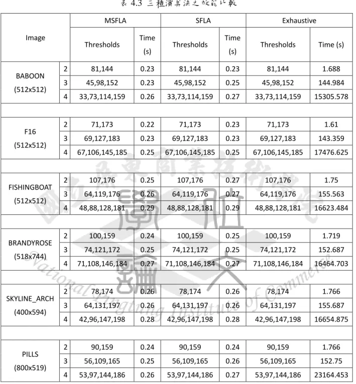
(11) 表目錄表 4.1 改良式混合蛙跳演算法對於醫學圖像之實驗結果...................................... 49 表 4.2 改良式混合蛙跳演算法對於測試圖像之實驗結果...................................... 50 表 4.3 三種演算法之效能比較.................................................................................. 51 表 4.4 支援向量機之參數優化實驗結果.................................................................. 52. viii.

(12) Chapter 1 緒論. 1.1 研究動機與目的 1.1.1 影像多閥值分割. 人類的眼睛可以很容易的從複雜的背景出分辨出物體，但對電腦而言卻是非常困難，要讓電腦能辨識物件需要對影像實行分析，其中包含非常多道的程序與技術，而其中的一步稱之為－影像分割 (Image segmentation)。. 影像分割，顧名思義能藉由切割影像取得需要的部分來執行後續處理，如同人類眼睛看見物體後大腦所運行的後端處理，對於電腦而言， “閥值(Thresholds)” 就是電腦的眼睛，藉由閥值進行的影像分割讓電腦能從圖片中分辨出物件，因此，影像閥值分割的優劣是讓電腦執行後續處理成功的關鍵。. 在影像閥值分割的演算法中會產生龐大的運算量(如全域搜尋法)，然而，現在的影像辨識技術已逐漸貼近人們的日常生活，相對於即時處理的需求與處理時間的標準也越來越高，因此，為了能解決此一問題，本研究導入了演化式運算，預期能在不失精準的情況下達到改善執行速度的效果。. 1.

(13) 1.1.2 支援向量機. 長久以來，”分類 (classification)” 一直是讓研究學者們高度關注的問題，原因在於其應用領域非常廣泛，如股市預測、醫學檢測、工業自動化流程檢測、人像辨識等，其中在為了解決這一問題而發展出了許多分類技術，如決策樹 (decision trees) 、倒傳遞神經網路 (back propagation neural networks) 、粗糙集理論 (rough set theory) 以及支援向量機 (support vector machines, SVM)。. 支援向量機是近年來經常被使用的一項分類技術，透過超平面 (Hyper plane) 的概念來適應並分類多維度的資料，概括來說，是藉由使用者輸入的資料，再透過”訓練 (training) ”這一過程來取得分類辨識的能力，在過程中會產生出支援向量機的關鍵參數”α”，這個參數將決定之後支援向量機的分類成功率。. 然而，輸入的訓練資料量越多雖然能更加地提升準確率，但在訓練的過程中會依據輸入的資料量產生相對應的高運算量，那將會是非常耗時的工程，為了改善這一缺點，本研究將導入演化式運算與支援向量機結合，試圖優化關鍵參數”α” 提升準確率，提升整體效率。. 2.

(14) 1.2 文獻探討 1.2.1 影像閥值影像閥值. 影像閥值技術主要可分為參數(parametric)或非參數(non-parametric)研究兩種，在參數研究中由於普遍認為灰階分佈較為接近高斯分佈，因此使用直方圖來找出最佳的解，但這通常都會造成非線性優化問題，使得運算成本變得昂貴且費時。非參數研究是基於以一個目標函數來搜尋最佳閥值，例如以均方差對影像作二值化的歐蘇法(Otsu’s function) [4]以及以熵值(entropy)為檢驗標準的方法 [5] 或是交叉熵(cross-entropy)檢驗法 [6]。. 當在進行閥值最佳化搜尋時的運算量是非常龐大且費時的，為了解決這個問題，近年來有許多學者與研究人員提出了導入演化式運算來搜尋最佳閥值的方法，如 K. Hammouche et al. [7] 以基因演算法 (Genetic algorithm, GA) 尋找出影像多閥值進行快速分割； M. Maitra et al. [8] 採用粒子群優化 (Particle Swarm Optimization, PSO) 執行影像多閥值分割；T.W. Jiang [9] 提出以蜜蜂生殖演算法 (Honey Bee Mating Optimization, HBMO) 應用於影像閥值與向量量化等。. 除了上述文獻所提出的方法之外，本研究將採用混合蛙跳演算法 (Shuffled frog-leaping optimization algorithm, SFLA) 以熵值最大化 (maximum entropy, MET) 為基準進行影像多閥值優化，在實驗中會對測試影像執行徹底的搜索並找出最佳解，同時檢測混合蛙跳演算法的收斂情形，最後在與全域搜尋法比較實驗結果。. 3.

(15) 1.2.2 支援向量機的應用與改進. 支援向量機是由貝爾實驗室研究人員 C. Cortes 與 V. Vapnik [10] 於 1995 年時所提出，是以結構風險最小化為基礎所發展出來的一套新方法，在發展過程中主要可分為線性支援向量機 (Linear support vector machines) 與非線性支援向量機 (Nonlinear support vector machines)。. 1998 年，C.J.C. Burges [11] 提出了一篇關於支援向量機的相關介紹與教程，使得當時尚未被廣泛運用的支援向量機開始走紅，時至今日，此項技術已成為現今最熱門的分類技術且被眾多領域廣泛應用，如 K. Jonsson et al. [12] 將支援向量機應用於臉部辨識、D.K. Iakovidis et al. [13] 應用於癌症前兆檢測、M. Awad et al. [14] 使用至視訊串流的動態分類上、M.C. Lee [15] 提出在股票趨勢預測上的應用、S. Tripathi et al. [16] 以降雨量評估氣候變化的影響等。. 除了在應用上的研究外，也有許多學者提出了以演化式運算加入到支援向量機中進行參數的優化實驗，如 C.L. Huang et al. [17] 將基因演算法用於支援向量機作參數優化；S.W. Lin et al. [18] 採用粒子群優化實現支援向量機優化來提高準確率、X.L. Zhang et al. [19] 以蟻群優化演算法實行支援向量機的參數優化等，在本研究中將採用近年來較新的演化式運算－混合蛙跳演算法 (Shuffled frog-leaping optimization algorithm) 導入至支援向量機中作為參數優化的方法，在實驗的過程中採用 UCI 的標準資料集合並進一步的測試優化結果，試圖改進支援向量機的參數優化問題。. 4.

(16) 1.3 研究方法簡介 1.3.1 演化式運算. 演化式運算是近年來非常重要的一項研究，從效率計算、視頻處理、氣象預測、經濟評估到工程領域都有所延伸，是一種能找到最佳近似解的一種方法。嚴謹的優化方法經常運用於線性規劃、動態規劃、分支限界技術以及到中等規模的問題上。然而，在現實生活中經常會遇到各種需要優化的問題，如工程實踐或是其他規模等問題，這些都是極富挑戰性的複雜運算，同時也是需要找出精確解的問題。. 演化式運算是一種隨機搜尋法，藉由模仿自然界生物的群聚行為、適應學習以及演化過程構築而成。最初這個方法是提出用來處理 NP-hard 問題時的解決方案，由於這類複雜問題需要大量的時間成本與高度的運算能力，因此為了克服這些問題，有研究人員提出了以演化式運算為基礎的方法，試圖尋找近似最佳解 [1]。. 在開發這類的計算方法時，研究人員模仿了各種生物的行為，如貓、鳥、蟑螂、螞蟻、蜜蜂、青蛙等，為高複雜度的優化問題尋求更快速且可靠的解。最早出現的演化式運算為基因演算法 (genetic algorithm) [2]，是一種嘗試減少執行時間、提高解質量與具有迴避局部最佳解特性的一種方法，然而在過去十年間已有許多應用與改善的相關研究，因此本研究將採用近年來所提出的一種新方法－混合蛙跳演算法 (Shuffled frog-leaping optimization algorithm)。. 5.

(17) 1.3.2 混合蛙跳演算法. 混合蛙跳演算法 (Shuffled frog-leaping algorithm) 是一種模因啟發式設計，用於尋找全域最佳解的搜尋法，在運算開始時會產生出複數隻青蛙 (solution) ，然後將每隻青蛙都會各自進行交換與全域交換的動作。所有的青蛙數量稱之為群集 (population,P)，然後依照群數 (memeplex,M) 進行分配，分配原則如圖 1.1，將第一隻放到第一群、第二隻放到第二群到第 M 隻放到第 M 群，而第 M+1 隻再放到第一群，依此類推。. 圖 1.1 混合蛙群演算法分群概念圖 6.

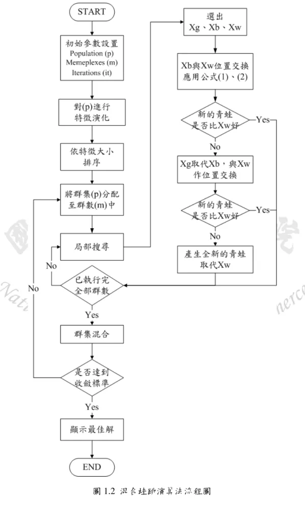
(18) 每一隻青蛙都會具有自己的特徵 (fitness)，依據特徵在每一群中分別選出最好的青蛙 (local best,X ) 與最差的青蛙 (local worst, X ) ，然後在從全部的青蛙之中選出最好的青蛙 (global best, X )。在每一次的演化的過程中，會依據以下公式來針對每一群中最好的青蛙與最差的青蛙來進行位置上的調整，公式如下：要交換的青蛙位置 D 新位置的青蛙. D. 其中. X. X. ∙ X. X. D ; D. D. D. (1.1) (1.2). 會產生 [0,1] 之間的隨機數、D 為青蛙之間要交換的位置量、. 則是青蛙之間位置交換量的最大限制。首先，在每一次的迭代中先將青蛙. 分群，之後先取出每群中最好的青蛙 (X ) 與最差的青蛙 (X ) 後代入公式 (1.1). 和 (1.2) 計算並比較取得的新的青蛙 (X ) 是否比原來那隻最差的青蛙(X )來得好，如果有的話就取代原本最差的青蛙 (X )，如果沒有，則把每一群中最好的青蛙(X )換成全域中最好的青蛙 (X ) ，然後再帶入公式 (1.1) 和 (1.2) 取得新的青蛙(X )並在跟原本最差的青蛙 (X ) 作比較看是否有比較好，如果有就取代原本最差的青蛙 (X )，如果還是沒有則將最差的青蛙捨棄，並以隨機的方式產生出新的青蛙來取代 [3]。. 當每一群中的青蛙都做完位置交換的動作後，就將所有的青蛙混合並依據特徵值由大到小重新排序，由此便可以取得全部青蛙中最好的青蛙 (global optimal solution) ，整體流程如圖 1.2。. 7.

(19) 圖 1.2 混合蛙跳演算法流程圖. 8.

(20) 1.3.3 改良式混合蛙跳演算法. 混合蛙跳演算法擁有粒子群優化 (Particle Swarm Optimization, PSO) 局部搜尋的特性，同時具備了全域最佳化參數搜尋法 (Shuffled Comlpex Evolution, SCE) 的資訊競爭能力，混合蛙跳演算法先讓每個個群獨立發展後再將其混合，藉此取得最好的青蛙 (solution)。. 除了原有的混合蛙跳演算法外，在近年來的研究中也有許多學者提出對混合蛙跳演算法進行改良的方法，其中一項研究就是針對上述公式 (1.1) 加上一個名為”搜尋-加速因子”的參數 C，如下：要交換的青蛙位置 D . ∙. ∙ X. X. (1.3). 加入這個參數的主要原因是因為原有的混合蛙跳演算法在局部搜尋時位置的交換幅度有時會太小，以致無法快速的找到最佳解，嚴重時甚至會導致無法找到最佳解，因此加入這個搜尋-加速因子 - C 來增加局部搜尋時的位置交換幅度以及提升混合蛙跳演算法的執行速度 [1]。. 1.4 論文結構簡介. 本論文在第二章時會介紹混合蛙跳演算法應用於影像多閥值優化時的流程，在第三章時會簡介支援向量機的基礎原理以及與混合蛙跳演算法結合的參數優化架構，第四章為影像多閥值優化與支援向量機參數優化的實驗結果，最後的第五章為結論。. 9.

(21) Chapter 2 運用混合蛙跳演算法於影像多閥值分割. 2.1 簡介. 影像多閥值優化 (Image thresholding optimization) 有許多可作為優化評定標準的方法，其中，本研究所採用的是熵值最大化 (maximum entropy) 作為優化評定的標準，在實驗中會以改良式混合蛙跳演算法、混合蛙跳演算法以及窮取法針對現實圖像進行分析並顯示結果。. 在混合蛙跳演算法的演化過程中，需要先為每隻青蛙制定作為特徵值的標準函數才能開始演化，不同的優化主題就會有不同的標準函數，而本研究在影像多閥值優化主題下所採用的是熵值最大化作為標準。. 2.2 熵值最大化與影像多閥值優化熵值最大化與影像多閥值優化. 本研究對於閥值最佳化的選取標準採用的是由 Kapur et al. [20] 於 1985 年所提出針對二值化閥值 (bi-level thresholding) 的熵值最大化度量法，而這個度量法也可延伸為多值化閥值 (multilevel thresholding) 方法。. 首先，取得目標圖像的灰階直方圖，最大範圍定義為 L ，因此其範圍表示為 {0, 1, …, L-1} 、影像的像素個數為 N ，像素機率函數的機率值則可定義為 ⁄ , 0. !. 1. (2.1). 10.

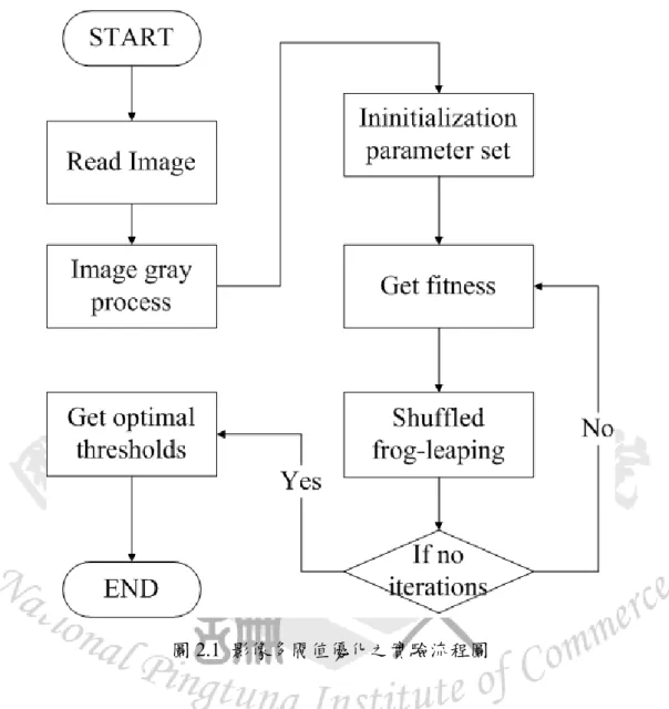
(22) 其中 h(i) 為灰階函數的分佈值、N 為目標圖像總像素，然而，若閥值數量. 有 c 個，則會有 [#$ , #% , …, #& ] 於熵值最大化函數中進行運算，公式如下： ' (#$ , #% , … , #& *. 1 2$ ∑03, , +,. .,. +,. +$. 1 2$ ∑0:3,. ; 2$ ∑030 , +$ 1. .$. < 2$ ∑030 ;. .%. ∑%>> 30?. .&. , +%. , +&. +%. ; 2$ ∑030 1. ⋮. 45. 67 45. 61. ln. ⋯. 45. 67. +&. ln 65 4. 1. 4 < 2$ 45 ∑030 ln 5 ; 6; 6;. ∑%>> 30?. 45. 6?. (2.2). ln 65 4. ?. 本研究所應用的改良式蛙跳演算法將以公式 (2.2) 所計算出的最大熵值為標準進行閥值優化。. 2.3 混合蛙跳演算法應用於影像多閥值優化. 本研究於混合蛙跳演算法應用於影像多閥值優化之實驗流程如圖 2.1。. Step 1. 初始參數設置. Population, P：群集，表示總體產生 n 組解集合，其中每一組解含有 c 個閥值，每個閥值介於 0 到下一個閥值之間，直到 L-1。 P = [ $,. %, … ,. ],. @#$ , #% , … , #& A, 0. #$. #%. ⋯. 11. #B. !. 1. (2.3).

(23) Memeplexes, M：群數，在每一次的迭代中會將 P 依序分配至每一群中，詳細流程請參照圖 1.1。 Iterations, it：迭代次數，決定演算法的總執行次數。本研究所設置參數為 P = 200、M = 10、it = 200。. Step 2. 取得特徵值. 每一組解會依據公式 (2.2) 計算相對應的適性值 (fitness, f )，藉此來作為評估每一組解的優劣好壞。. Step 3. 青蛙跳. 在此步驟中，會依照群數 M 來參考公式 (1.1) 與 (1.2) 執行每一組解的汰換程序，首先會取出第一群中最佳與最差的解進行運算，若產生的新解比原有的最差解要好就將之取代，若沒有，則換成全域最佳解與當下群中的最差解進行運算，若產生的新解較好則取代，若還是沒有則將原有的最差解捨棄，重新隨機產生一組解放置回群集，其中以改良式蛙跳演算法執行時所使用的搜尋加速因子”C”為產生 [1,2] 之間的隨機數來增加搜尋效果，詳細流程請參照圖 1.2。. Step 4. 混合排序. 將迭代完的全部解重新混合並依序由大到小排列，由此取得最佳解。. Step 5 終止條件確認檢查是否已達終止條件，若為是則顯示最佳解，否則回到 Step 2 繼續執行。. 12.

(24) 圖 2.1 影像多閥值優化之實驗流程圖. 在取得最佳閥值後會計算峰值訊噪比 (Peak Signal to Noise Ratio, PSNR) 作為多閥值影像分割的效能評估，單位為 dB，其計算式如下： C D. 20log$,. 255 DICJ. (2.4). 其中，RMSE 為均方根誤差 (Root Mean Square Error, RMSE) ，運算如下： DICJ. K. ∑P3$ ∑N O3$ L , M I. L ,M. %. 在公式 (2.5) 中，I 跟 L 是原始圖像與分割後的圖像，I Q. 13. (2.5) 為圖像大小。.

(25) Chapter 3 運用混合蛙跳演算法於非線性支援向量機之參數優化運用混合蛙跳演算法於非線性支援向量機之參數優化 3.1 簡介支援向量機的發展已有一段時日，在過去十年間逐漸成熟，同時也受到眾多領域的廣泛應用，這項技術是透過 VC 維 (Vapnik Chervonenkis dimension) 與結構風險最小化 (Structural risk minimization) 的概念所開發而成的分類工具，後續的發展中主要可分為兩種：線性 (linear) 與非線性 (nonlinear) 的支援向量機。. 3.2 線性支援向量機. 支援向量機是利用一個超平面 (hyperplane) 概念來進行分類的一項技術，需要經過”訓練 (training)”這一過程後才能開始進行分類，其中訓練的資料集合. 可定義為 {R , S }，i = 1, 2, …, m，R ∈ UV ，S ∈ W 1, 1X，當資料位於超平面時，可用下列式子表示： Y∙R Y∙R. Z[ Z. 1 1. for S for S. 1. (3.1). 1. (3.2). 公式 (3.1) 與 (3.2) 表示為超平面上的直線方程式，其中 w 為向量、b 為偏移量，其概念如圖 3.1，為了達到超平面的最佳化，就必須滿足以下條件使區間 (Margin) 最大化，如公式 (3.3)： \ S Y∙R. I. ‖Y‖ _ 2 Z 1 [ 0 ∀. (3.3). 14.

(26) 圖 3.1 SVM 分類概念圖由於上述公式 (3.3) 並沒有封閉解，因此導入拉格朗日多項式乘數. (Lagrange’s multipliers) 試圖取得近似最佳解 ` ,. 式 (3.4). Iab： !c ` ` [ 0,. 1, … ,. e. d` 3$. 1, … ,. 並使其最大化，如公. N. 1 d ` `O S SO R RO 2 ,O3$. ∑N3$ ` S. 0. (3.4). 最後，藉由公式 (3.4) 訓練後找出最佳化超平面來進行分類；但是，一般來說，以線性方式就能將資料完全分離是非常罕見的，大多數的情況都是無法分類完全，因此為了因應此一問題，便衍生出了非線性支援向量機。. 15.

(27) 3.3 非線性支援向量機. 在現實情況中，要維持原始維度來進行分類其實是很困難的，因此為了解決這一難點，便延伸出了非線性的分類方法，稱之為－非線性支援向量機 (Non-Linear Support Vector Machines)。. 與線性支援向量機不同的是，非線性支援向量機在尋找超平面前會先將資料投射到特徵空間，其概念如圖 3.2：. 圖 3.2 特徵空間投射概念圖其表示式為. 或表示為. Φ：UV ↦ h. (3.5). R→Φ R. (3.6). 16.

(28) 在將訓練資料投射至更高維度後將使得運算式會變得很繁雜並耗費大量資源與時間進行內積運算，因此為了減少計算量與加快處理速度，便定義了核心函數 (kernel function)： j R , RO. Φ R ∙ Φ RO. (3.7). 如公式 (3.7) ，其中 K 函數被稱之為核心函數，再將公式 (3.4) 與 (3.7) 結合後可得 e. Iab： !c `. ` [ 0,. 其中. N. d` 3$. 1, … ,. 1 d ` `O S SO j R , RO 2 ,O3$. ∑N3$ ` S. (3.8). 0. 在經過公式 (3.8) 的訓練後取得 ` ，方能找到相對應的可分離超平面，如. 公式 (3.9) ，其中會有偏差值隱含所應用的核心函數之中，因此設立一偏差條件，如果符合條件才於予採用，如公式 (3.10) ，被採用的向量稱之為－支援向量 (support vector, SV)。 ' R, ` , Z ∗. ∗. ' R, ` ∗ , Z ∗. N. d S `∗j R , R 3$ N. d S `∗j R , R 3$. Z∗ Z∗. (3.9) d S ` ∗j R , R ∈lm. (3.10). 定義核心 K 函數除了方便計算外，更能讓使用者定義更多的核心函數來應用在 SVM 上，以下介紹幾個常見的核心函數：線性核心函數 ( Linear kernel function )： jnR , RO o. R ∙ RO. (3.11). 多項式核心函數 ( Polynomial kernel function )： jnR , RO o. R ∙ RO. 1. V. with d ∈ N. 17. (3.12).

(29) 高斯徑向基核心函數 ( Gaussian radial basis function )： jnR , RO o. p 2qrs5 2str. ;. (3.13). 正切雙曲線核心函數 ( Tangent hyperbolic kernel function )： jnR , RO o. tanh R ∙ RO. Θ. (3.14). 3.4 混合蛙跳演算之參數優化 3.4.1 實驗設計. 支援向量機主要可分為特徵選取 (feature selection) 與參數優化 (parameters optimization) 兩種改良方式，本研究採用混合蛙跳演算法針對參數優化進行改良，在實驗開始前，首先需要設計每一隻青蛙身上所具備的參數，由於本研究使用高斯徑向基函數作為核心函數，因此除了原有定義的 ` 之外，還需要定義 y 一同訓練優化，而公式 (3.8) 的運算值則作為青蛙跳時的淘汰標準。 'z$. '{$. ' $1. ……. ' $|. ….. 'z. 圖 3.3 青蛙參數設計圖. '{. '1. ……. 與. '|. 如圖 3.3， 'z$ 、'{$ 為第一組解的 C 參數跟 y 參數， ' $1 …' $| 為第一組. 的 ` 向量值，直到第 n 隻青蛙。. 3.4.2 實驗流程. 本研究的實驗是基於混合蛙跳演算法與支援向量機的參數優化建構而成，其實驗流程如圖 3.4。. 18.

(30) 資料處理. Step 1. 資料處理主要分為兩個步驟，正規化與 k-fold ，正規化的主要目的是避免較大的值去影響較小的值而導致資料的不均性，因此本研究在實驗開始前先將輸入資料進行正規化的步驟，其正規化後的資料範圍在 [+1, -1] ，公式如下： } ~ ~ • ~. }. (3.15). 正規化後接著要進行 k-fold [21] 將資料切割為訓練資料與測試資料，在本研究中 k 值設為 10 ，也就是分成 10 個部分，其中一份作為測試，剩餘九份作為測試，例如第一部分作為測試資料、其他第二到十份作為訓練，接著第二部分作為測試、第一及第三到十部分作為測試，依此類推。. Step 2. 參數初始化. 在訓練開始前必須要設置初始參數後才能開始進行迭代演化，依據圖 3.3 設 $. 置參數，全部參數皆由隨機產生，其中 C 的產生範圍設置在 [2$> ,%1€ ] 、y 的. 參數產生範圍在 [2> ,%€ ] 、` 則依據公式 (3.8) 的 0 $. `. ,. 1, … ,. 範圍. 隨機產生。. Step 3. 混合蛙跳演算法. 在此步驟中會依據圖 1.2 中的混合蛙跳演算流程進行參數優化，每一次的汰. 換中都會藉此更新 C、y 以及 ` 參數，其中群集設置為 100 、群數設置為 10 ，. 迭代次數為 200，然後依據結果選出最佳解。. Step 4. 優化分類器測試. 在取得優化的參數之後在對測試資料進行測試，由於本研究的 k 值設為 10，因此在執行完 10 次後取得分類成功率，在取得平均值後顯示結果。. 19.

(31) 圖 3.4 SVM 參數優化之實驗流程圖. 20.

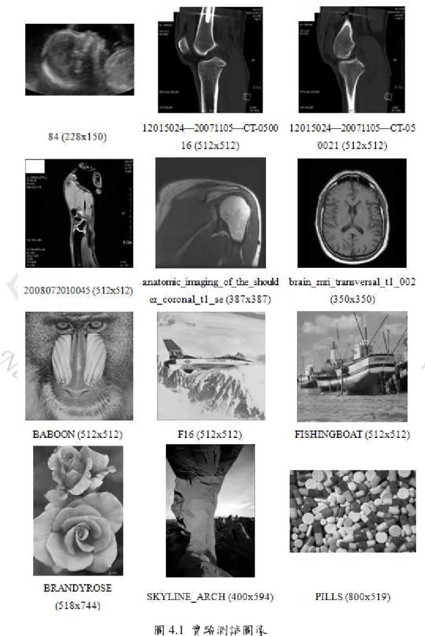
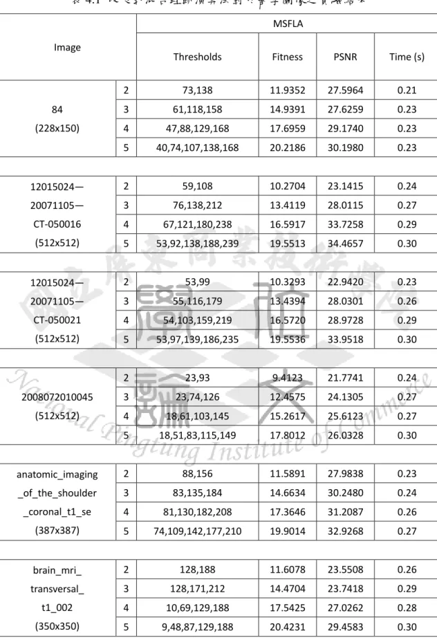
(32) Chapter 4 實驗結果. 4.1 研究環境簡介. 本研究所使用的環境是 Intel Pentium D 2.80 GHz CPU 、 512 MB RAM 、作業系統為 Microsoft Windows XP Professional Version 2002 SP 3 、開發軟體為 Microsoft Visual Studio 2008。. 4.2 影像多閥值優化實驗結果. 本研究實驗中所使用的測試圖像如圖 4.1，其中六種是標準測試圖像，分別為 ” BABOON” 、 ” F16” 、 ” FISHINGBOAT” 、 ” BRANDYROSE” 、 ” SKYLINE_ARCH” 、 ” PILLS” ，另外六種為醫學圖像則是 ” 84” 、 ” 12015024—20071105—CT-050016”、 ” 12015024—20071105—CT-050021”、 ” 2008072010045” 、. ” anatomic_imaging_of_the_shoulder_coronal_t1_se” 、. ”. brain_mri_transversal_t1_002”。. 圖 4.2 – 4.13 分別為各個圖像的多閥值優化結果，圖 4.14 – 4.17 表示為 Baboon 與 F16 圖像於多閥值分割實驗中的收斂情形，表 4.1 是改良式混合蛙跳演算法對於醫學圖像的實驗結果，表 4.2 則是應用於測試圖像的優化結果，最後表 4.3 為窮取法、混合蛙跳演算法、改良式混合蛙跳演算法的分別比較結果。. 21.

(33) 圖 4.1 實驗測試圖像. 22.

(34) Original image. Histogram. 2-level thresholding image. The selected thresholds of 2-level threshold. 3-level thresholding image. The selected thresholds of 3-level threshold. 23.

(35) 4-level thresholding image. The selected thresholds of 4-level threshold. 5-level thresholding image. The selected thresholds of 5-level threshold. 圖 4.2 84 圖像優化閥值切割結果. 24.

(36) Original image. Histogram. 2-level level thresholding image. The selected thresholds of 2-level level threshold. 3-level level thresholding image. The selected thresholds of 3-level evel threshold. 25.

(37) 4-level thresholding image. The selected thresholds of 4-level threshold. 5-level thresholding image. The selected thresholds of 5-level threshold. 圖 4.3 12015024—20071105—CT-050016 圖像優化閥值切割結果. 26.


(39) 4-level thresholding image. The selected thresholds of 4-level threshold. 5-level thresholding image. The selected thresholds of 5-level threshold. 圖 4.4 12015024—20071105—CT-050021 圖像優化閥值切割結果. 28.


(41) 4-level thresholding image. The selected thresholds of 4-level threshold. 5-level thresholding image. The selected thresholds of 5-level threshold. 圖 4.5 2008072010045 圖像優化閥值切割結果. 30.


(43) 4-level thresholding image. The selected thresholds of 4-level threshold. 5-level thresholding image. The selected thresholds of 5-level threshold. 圖 4.6 anatomic_imaging_of_the_shoulder_coronal_t1_se 圖像優化閥值切割結果. 32.


(45) 4-level thresholding image. The selected thresholds of 4-level threshold. 5-level thresholding image. The selected thresholds of 5-level threshold. 圖 4.7 brain_mri_transversal_t1_002 圖像優化閥值切割結果. 34.


(47) 4-level thresholding image. The selected thresholds of 4-level threshold. 5-level thresholding image. The selected thresholds of 5-level threshold. 圖 4.8 BABOON 圖像優化閥值切割結果. 36.


(49) 4-level thresholding image. The selected thresholds of 4-level threshold. 5-level thresholding image. The selected thresholds of 5-level threshold. 圖 4.9 F16 圖像優化閥值切割結果. 38.


(51) 4-level thresholding image. The selected thresholds of 4-level threshold. 5-level thresholding image. The selected thresholds of 5-level threshold. 圖 4.10 FISHINGBOAT 圖像優化閥值切割結果. 40.


(53) 4-level thresholding image. The selected thresholds of 4-level threshold. 5-level thresholding image. The selected thresholds of 5-level threshold. 圖 4.11 BRANDYROSE 圖像優化閥值切割結果. 42.


(55) 4-level thresholding image. The selected thresholds of 4-level threshold. 5-level thresholding image. The selected thresholds of 5-level threshold. 圖 4.12 SKYLINE_ARCH 圖像優化閥值切割結果. 44.


(57) 4-level thresholding image. The selected thresholds of 4-level threshold. 5-level thresholding image. The selected thresholds of 5-level threshold. 圖 4.13 PILLS 圖像優化閥值切割結果. 46.

(58) Number of optimal frog replaced in iterations. 80 70 60 50 T=2. 40. T=3 30. T=4 T=5. 20 10 0 0. 20. 40. 60. 80. 100 120 140 160 180 200. Number of iterations. 圖 4.14 Baboon 收斂實驗曲線圖 (MSFL). Number of optimal frog replaced in iterations. 120. 100. 80 T=2. 60. T=3 T=4. 40. T=5 20. 0 0. 20. 40. 60. 80. 100 120 140 160 180 200. Number of iterations. 圖 4.15 Baboon 收斂實驗曲線圖 (SFL). 47.

(59) Number of optimal frog replaced in iterations. 80 70 60 50 T=2. 40. T=3 30. T=4 T=5. 20 10 0 0. 20. 40. 60. 80. 100 120 140 160 180 200. Number of iterations. 圖 4.16 F16 收斂實驗曲線圖 (MSFL). Number of optimal frog replaced in iterations. 100 90 80 70 60 T=2. 50. T=3 40. T=4. 30. T=5. 20 10 0 0. 20. 40. 60. 80. 100 120 140 160 180 200. Number of ierations. 圖 4.17 F16 收斂實驗曲線圖 (SFL). 48.

(60) 表 4.1 改良式混合蛙跳演算法對於醫學圖像之實驗結果 MSFLA Image Thresholds. Fitness. PSNR. Time (s). 2. 73,138. 11.9352. 27.5964. 0.21. 84. 3. 61,118,158. 14.9391. 27.6259. 0.23. (228x150). 4. 47,88,129,168. 17.6959. 29.1740. 0.23. 5. 40,74,107,138,168. 20.2186. 30.1980. 0.23. 12015024—. 2. 59,108. 10.2704. 23.1415. 0.24. 20071105—. 3. 76,138,212. 13.4119. 28.0115. 0.27. CT-050016. 4. 67,121,180,238. 16.5917. 33.7258. 0.29. (512x512). 5. 53,92,138,188,239. 19.5513. 34.4657. 0.30. 12015024—. 2. 53,99. 10.3293. 22.9420. 0.23. 20071105—. 3. 55,116,179. 13.4394. 28.0301. 0.26. CT-050021. 4. 54,103,159,219. 16.5720. 28.9728. 0.29. (512x512). 5. 53,97,139,186,235. 19.5536. 33.9518. 0.30. 2. 23,93. 9.4123. 21.7741. 0.24. 2008072010045. 3. 23,74,126. 12.4575. 24.1305. 0.27. (512x512). 4. 18,61,103,145. 15.2617. 25.6123. 0.27. 5. 18,51,83,115,149. 17.8012. 26.0328. 0.30. anatomic_imaging. 2. 88,156. 11.5891. 27.9838. 0.23. _of_the_shoulder. 3. 83,135,184. 14.6634. 30.2480. 0.24. _coronal_t1_se. 4. 81,130,182,208. 17.3646. 31.2087. 0.26. (387x387). 5. 74,109,142,177,210. 19.9014. 32.9268. 0.27. brain_mri_. 2. 128,188. 11.6078. 23.5508. 0.26. transversal_. 3. 128,171,212. 14.4704. 23.7418. 0.29. t1_002. 4. 10,69,129,188. 17.5425. 27.0262. 0.28. (350x350). 5. 9,48,87,129,188. 20.4231. 29.4583. 0.30. 49.

(61) 表 4.2 改良式混合蛙跳演算法對於測試圖像之實驗結果 MSFLA Image Thresholds. Fitness. PSNR. Time (s). 2. 81,144. 12.2177. 24.4816. 0.23. BABOON. 3. 45,98,152. 15.2792. 25.1922. 0.23. (512x512). 4. 33,73,114,159. 18.1263. 26.4155. 0.26. 5. 33,70,105,139,173. 20.7888. 28.5242. 0.27. 2. 71,173. 12.2114. 23.6582. 0.22. F16. 3. 69,127,183. 15.5039. 26.7103. 0.23. (512x512). 4. 67,106,145,185. 18.3119. 28.2423. 0.25. 5. 60,90,125,157,188. 20.9086. 29.2181. 0.26. 2. 107,176. 12.5748. 23.4688. 0.25. FISHINGBOAT. 3. 64,119,176. 15.8209. 25.7827. 0.26. (512x512). 4. 48,88,128,181. 18.6557. 26.6927. 0.29. 5. 48,88,128,174,202. 21.4016. 27.6536. 0.29. 2. 100,159. 12.2736. 24.9256. 0.24. BRANDYROSE. 3. 74,121,172. 15.2595. 26.1420. 0.25. (518x744). 4. 71,108,146,184. 18.7017. 28.1049. 0.27. 5. 71,107,143,179,220. 20.7612. 28.4059. 0.29. 2. 78,174. 12.6668. 23.1858. 0.26. SKYLINE_ARCH. 3. 64,131,197. 16.0391. 25.5107. 0.26. (400x594). 4. 42,96,147,198. 19.1042. 26.9944. 0.28. 5. 32,71,114,158,203. 21.96716. 28.2495. 0.29. 2. 90,159. 12.6897. 24.4658. 0.24. PILLS. 3. 56,109,165. 15.8172. 24.8348. 0.25. (800x519). 4. 53,97,144,186. 18.7259. 27.2353. 0.26. 5. 51,94,140,183,234. 21.5477. 27.2712. 0.30. 50.

(62) 表 4.3 三種演算法之效能比較 MSFLA Image Thresholds. BABOON (512x512). F16 (512x512). FISHINGBOAT (512x512). BRANDYROSE (518x744). SKYLINE_ARCH (400x594). PILLS (800x519). SFLA Time (s). Thresholds. Exhaustive Time (s). Thresholds. Time (s). 2. 81,144. 0.23. 81,144. 0.23. 81,144. 1.688. 3. 45,98,152. 0.23. 45,98,152. 0.25. 45,98,152. 144.984. 4. 33,73,114,159. 0.26. 33,73,114,159. 0.27. 33,73,114,159. 15305.578. 2. 71,173. 0.22. 71,173. 0.23. 71,173. 1.61. 3. 69,127,183. 0.23. 69,127,183. 0.23. 69,127,183. 143.359. 4. 67,106,145,185. 0.25. 67,106,145,185. 0.25. 67,106,145,185. 17476.625. 2. 107,176. 0.25. 107,176. 0.27. 107,176. 1.75. 3. 64,119,176. 0.26. 64,119,176. 0.27. 64,119,176. 155.563. 4. 48,88,128,181. 0.29. 48,88,128,181. 0.29. 48,88,128,181. 16623.484. 2. 100,159. 0.24. 100,159. 0.25. 100,159. 1.719. 3. 74,121,172. 0.25. 74,121,172. 0.25. 74,121,172. 152.687. 4. 71,108,146,184. 0.27. 71,108,146,184. 0.27. 71,108,146,184. 16464.703. 2. 78,174. 0.26. 78,174. 0.26. 78,174. 1.766. 3. 64,131,197. 0.26. 64,131,197. 0.26. 64,131,197. 155.687. 4. 42,96,147,198. 0.28. 42,96,147,198. 0.28. 42,96,147,198. 16654.875. 2. 90,159. 0.24. 90,159. 0.24. 90,159. 1.766. 3. 56,109,165. 0.25. 56,109,165. 0.26. 56,109,165. 152.75. 4. 53,97,144,186. 0.26. 53,97,144,186. 0.27. 53,97,144,186. 23164.453. 51.

(63) 4.3 支援向量機之參數優化實驗結果. 本研究在支援向量機之參數優化的實驗中所採用的是 UCI dataset [22] 進行實驗測試，分別是” SPECTF”、 ” WDBC”、 ” Heart disease”、 ” German”、 ” Sonar”、 ” pima”、 ” Australian”、 ” bupa live”、 ” Ionosphere”、 ” Breast cancer”，實驗結果如表 4.4。. 表 4.4 支援向量機之參數優化實驗結果 Data from UCI Machine Learning Repository Dataset. No. of. No. of. No. of. class. instances. features. Accuracy. 1. SPECTF. 2. 267. 44. 0.769231. 2. WDBC. 2. 569. 30. 0.9625. 3. Heart disease (StatlogProject). 2. 270. 13. 0.792593. 4. German (Credit card). 2. 1000. 24. 0.686. 5. Sonar. 2. 208. 60. 0.86. 6. pima-indians-diabetes. 2. 768. 8. 0.725. 7. Australian (Credit card). 2. 690. 14. 0.8376871. 8. bupa live. 2. 345. 6. 0.62029. 9. Ionosphere. 2. 351. 34. 0.868571. 2. 699. 10. 0.965217. 10 Breast cancer (Wisconsin). 52.

(64) Chapter 5 研究結論與未來展望. 本研究以近年來較新的混合蛙跳演算法嘗試應用於影像多閥值與支援向量機之參數優化上，在影像多閥值方面，從實驗中可以得知以熵值最大化為度量標準所搜尋出的優化閥值與全域搜尋法結果相同，但效能卻有大幅度的提升；在支援向量機之參數優化的實驗中，部分資料集的測試結果良好，但其他測試資料則稍有落差，此部分的詳細過程尚須探討。. 在未來，本研究將針對支援向量機參數優化不足之處進行改良，並改為多分類參數優化。. 53.

(65) 參考文獻. [1] E. Elbeltagi, T. Hegazy, D. Grierson, “A modified shuffled frog-leaping optimization algorithm: applications to project management”, Structure and Infrastructure Engineering, Vol. 3, No. 1, March 2007, 53-60. [2] J.H. Holland, “Adaptation in natural and artificial systems”, University of Michigan Press: Ann Arbor, 1975. [3] M.M. Eusuff, K.E. Lansey, “Optimization of Water Distribution Network Design using the Shuffled Frog Leaping Algorithm”, Journal of Water Resources Planning and Management, Vol. 129, No. 3, May/June 2003, 210-225. [4] N. Otsu, “A threshold selection method for grey level histograms”, IEEE Trans. Syst. Man Cybernet. SMC-9 (1979), 62–66. [5] T. Pun, “A new method for grey-level picture thresholding using the entropy of the histogram”, Signal Processing, Vol. 2, Issue 3, July 1980, 223-237. [6] M. Sezgin, B. Sankur, “Survey over image thresholding techniques and quantitative performance evaluation”, Journal of Electronic Imaging, Vol. 13, No. 1, January 2004, 146-165. [7] K. Hammouche, M. Diaf, P. Siarry, “A multilevel automatic thresholding method based on a genetic algorithm for a fast image segmentation”, Computer Vision Graphics and Image Understanding 109 (2008), 163-175. [8] M. Maitra, A. Chatterjee, “A hybrid cooperative–comprehensive learning based PSO algorithm for image segmentation using multilevel thresholding”, Expert Systems with Applications 34 (2008) 1341–1350.. 54.

(66) [9] T.W. Jiang, “The Application of Image Thresholding and Vector Quantization Using Honey Bee Mating Optimization”, Master thesis of National PingTung Institute of Commerce, Taiwan, 2009. [10] C. Cortes, V. Vapnik, “Support-Vector Networks”, Machine Learning 20 (1995), 273-297. [11] C.J.C. Burges, “A Tutorial on Support Vector Machines for Pattern Recognition”, Data Mining and Knowledge Discovery 2, 1998, 121-167. [12] K. Jonsson, J. Kittler, Y.P. Li, J. Matas, “Support vector machines for face authentication”, Image and Vision Computing, Vol. 20, Issues 5-6, 15 April 2002, 369-375. [13] D.K. Iakovidis, D.E. Maroulisa, S.A. Karkanisb, P. Papageorgasa, M. Tzivras, “Texture multichannel measurements for cancer precursors’ identification using support vector machines”, Measurement, Vol. 36, Issues 3–4, October–December 2004, 297–313. [14] M. Awad, Y. Motai, “Dynamic classification for video stream using support vector machine”, Applied Soft Computing, Vol. 8, Issue 4, September 2008, 1314–1325. [15] M.C. Lee, “Using support vector machine with a hybrid feature selection method to the stock trend prediction”, Expert Systems with Applications 36 (2009) 10896–10904. [16] S. Tripathi, V.V. Srinivasa, R.S. Nanjundiah, “Downscaling of precipitation for climate change scenarios: A support vector machine approach”, Journal of Hydrology 330 (2006) 621–640. [17] C.L. Huang, C.J. Wang, “A GA-based feature selection and parameters optimization for support vector machines”, Expert Systems with Applications 31 (2006) 231–240. 55.

(67) [18] S.W. Lin, K.C. Ying, S.C. Chen, Z.J. Lee, “Particle swarm optimization for determination and feature selection of support vector machines”, Expert Systems with Applications 35 (2008) 1817–1824. [19] X.L. Zhang, X.F. Chen, Z.J. He, “An ACO-based algorithm for parameter optimization of support vector machines”, Expert Systems with Applications, Volume 37, Issue 9, September 2010, Pages 6618-6628. [20] J.N. Kapur, P.K. Sahoo, A.K.C. Wong, “A new method for gray-level picture thresholding using the entropy of the histogram”, Computer Vision Graphics and Image Understanding 29 (1985), 273-285. [21] S.L. Salzberg, “On comparing classifiers: Pitfalls to avoid and a recommended approach”, Data Mining and Knowledge Discovery 1 (1997), 317-327. [22] D. J. Newman, S. Hettich, C. L. Blake, and C. J. Merz, “UCI Repository of Machine Learning Databases,” Department of Information and Computer Science, University of California, Irvine, 1998.. 56.

(68)