A review of scatter correction methods for three-dimensional positron emission tomography

1,2 2 2

1 2

94ѐ8͡23͟צந 94ѐ9͡27࣒͟Լ 94ѐ9͡28͟ତצΏྶ

ᓑඛˠĈӓڔ౾̀ έ̚ξ406Δ͏ડ ֧̄ ̄ޒ11ཱི ̚έࡊԫ̂ጯٸडԫఙր

࿪ྖĈ0928246662 ็ৌĈ(03) 4891792 ࿪̄ܫቐĈ[email protected]

(PET)

septa

(coincident events)

50% PET

ᙯᔣෟĈ

८̄ᗁᄫ2005;18:225-233

݈֏

ᐌ ඾ Ϡ ᗁ ̶ ̄ ᇆ ည ۞ ൴ ण Ă ϒ ̄ ࿪ ཝ ᕝ ᆸ ౄ ᇆ

(positron emission tomography; PET) Яࠎ׍౯੼ីୂޘᄃ

࿪ཝᕝᆸౄᇆ۞ؠณপّਕឰᇆညࢦޙޢ̝វ৵ࣃ΃ܑ

߿វ̚Ԋొٸडّ८჌፧ޘ۞඗၆ณĂ่̙Ξϒቁ۞ቁ

ܲ׎ۏநຍཌྷ֭೩ֻᓜԖ۞ˠវྤੈĂՀΞӀϡᇾᆽᘽ ۏдវ̰ᐌ඾ॡԔត̶̼̝ҶĂෞҤ׎ᘽநણᇴĂͽΐ

ిາᘽ۞ฟ൴Ą൒҃ĂϤٺϒ̄࿪ཝᕝᆸౄᇆߏӀϡ௑

Ъ (coincidence) ઍീ۞ࣧநֽјညĂ׎̚хдధкሕд ણᇴ኏ᑝPETณീ۞໤ቁّĂ఺ֱЯ৵Β߁ઍᑭጡ۞൑

ຏॡมड़ᑕ (dead time effect) ౄј۞ࢍᇴதຫεăઍᑭጡ ड़தត̼ăਕ඄̂̈నؠăᐌְ፟Іड़ᑕă௡ᖐ਽ഴड़ ᑕᄃ೸डड़ᑕඈĄ

ϒ̄дវ̰ᄃ࿪̢̄໑யϠ511 keV۞Ѝ̄Ă౵Ξਕ ᄃ௡ᖐயϠ۞Ϲ̢үϡߏ૵೼ӌ೸ड (Compton scatter-

ing)ĂЍ̄ົᖼொొЊਕณග௡ᖐ̚۞࿪֭̄ͷயϠ֎ޘ

۞ઐԶĄ௑ЪְІܮ̙Г၆ᑕٺࣧώ۞਽តҜཉĂซ҃

ౄј८჌Ҝཉ۞᏾ҤĂࢫҲ˞ؠณ۞໤ቁّĄѩγĂॲ ፂҹֽЯů̥ࡊ (Klein Nishina) ̳ё [1]Ă༊೸डЍ̄ઐ Զ֎ޘ̈ٺ45ޘॡĂΞਕΪᖼொ115 keV۞ਕณග̟аྯ

࿪̄Ă̪֭ܲѣ396 keVĄފٺPETઍᑭጡ۞ਕณྋژޘ ࢨט (15%~30% FWHMд511 keV)â࣎Βӣ೸डүϡ

۞௑ЪְІޝΞਕ̪൒జ͹ਕ඄ (350~650 keV) ତצĂЯ ѩĂ̙टٽӀϡਕ඄̶ֽ࿣೸ड௑ЪְІᄃϏ೸डְ

ІĂซ҃ౄјᇆညݡኳ۞ሀቘᄃؠณ໤ቁޘ۞ࢫҲĄ дٙତќז۞௑ЪְІ̝̚Ă૵೼ӌ೸डٙҫ۞ͧ

ּჍࠎ೸ड̶தĂ׎̂̈פՙٺᇴ࣎ણᇴĂΒӣ೸डۏ វ۞̂̈ᄃ૜ޘăPETବೡጡ۞ೀңඕၹăਕ඄ቑಛ ඈĄ˟ჯPET۞೸ड̶தࡗࠎ15% (ѣinter-slice septa)Ă Ӏϡseptaֽ֨ͤҋ׎΁πࢬ۞೸डԛј୆Ш۞LOR (line

of response)ĂЯѩਕѣड़ࢫҲ೸डְІĂҭ˵࠹၆ᜁࠗ

˞͹ࢋְІ۞ីୂޘĄܕѐֽࠎ˞ᆧΐր௚ីୂޘĂ૱

૟septa྅ཉொੵĂͽᕜפྭπࢬ (cross plane) ۞͹ࢋְ

ІĂჍࠎˬჯሀёĂ׎೸ड̶த˘ਠౌ੼྿30~50%

[2]Ăٙͽдˬჯϒ̄࿪ཝᕝᆸౄᇆր௚̚Ăтңѣड़ঐ

ੵ೸डְІࠎԼචޢᜈ۞ؠณඕڍ۞ࢦࢋᙯᔣĄ

೸डᒣϒ

ᔵ൒ೡ̢ࢗ໑Ѝ̄யϠ૵೼ӌ೸ड۞ۏநপّᅲࠎ ኑᗔĂҭѣೀ࣎LOR۞পّΞͽϡֽෞҤ׎೸ड̶ҶĂ

֭೩ֻ೸डᒣϒ۞ΞਕّĈ(1) дۏវγLORٙ੃ᐂז۞

ְІᇴкࠎ೸डְІĂЯࠎ͹ࢋְІ (primary event) ԛ ј۞LOR˘ؠົజԊࢨдۏវ̰ (઄నᐌְ፟І̏གྷజ

ொੵ)ć(2) ೸ड̶Ҷߏ˘࣎ត̼ቤၙ۞בᇴĂͷ̙׍۩

มྤੈć(3) дਕᙉ̚ĂҲٺ͹ࢋਕ඄ਕณ۞ְІ̂ొ̶

ࠎ೸डְІć(4) ೸डְІࡶརд͹ਕ඄̰ĂкΗֽҋಏ Ѩ೸डĄॲፂ఺ֱ̙Т۞পّࢉϠ΍ЧёЧᇹ۞೸डᒣ ϒ͞ڱĂ͹ࢋડ̶ࠎ׌̂ቑᘞĈ(1) ॲፂٙ଀Ըᇆྤੈ࿰

ീ೸ड̶ҶĂּтĈ̰೧૜Ъڱ (curve fitting method)ă ਕ඄ૄغڱ (energy-baesd method)ăଡ᎕ഴᖴڱ (convo-

lution subtraction method)ć(2) ͽࢦޙޢᇆညࠎૄᖂ۞೸

ड࣒ϒڱĂּтĈሀё᎕غڱ (model-based method)ăࢦ ޙૄغڱ (reconstruction-based method)Ą

ѩγĂܕѐֽԧࣇࡁ൴΍डՁܡጿ྅ཉڱ (beam-

stopper method) ͽซҖ೸डᒣϒĄѩᄃ݈ࢗ͞ڱ͹ࢋम

̰೧૜Ъڱ

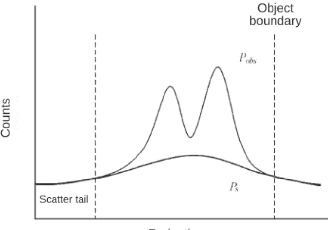
ѩᙷ೸डᒣϒڱ [3,4] ߏӀϡԸᇆྤफ़̚ۏវγ೸ड

۞ณͽᑢЪྋژ͞඀ёĂтFigure 1ٙϯĂͽ˟Ѩкีё

ٕߏ੼೻̳ёֽᑢЪᙝቡ۞೸डԍ͐ (P_s

)Ąѩڱ͹ࢋߏ

ॲፂ၁ᅫ۞៍ീྤफ़ (P_obs

)Ă֭઄నдۏវγజ੃ᐂ۞௑

ЪְІБొౌֽҋٺ೸ड (઄నᐌְ፟І̏ԆБజொੵ

۞݈೩˭)Ă֭ͷ೸ड̶Ҷࠎ˘ҲᐛבᇴĄѩ͞ڱਕѣड़

࣒ϒֽҋFOV (field of view) γ۞೸ड੒ᚥĂͷ׍ѣങˢ ᖎಏᄃ੼ࢍზड़த̝ᐹᕇĄ͹ࢋ৿ᕇࠎ೸ड̶Ҷ̙֍଀

Ξͽϡπ໣۞בᇴֽܕҬĂ͍׎д਒ටౄᇆĂ௡ᖐ૜ޘ ត̼ܧ૱̂ĂΞਕົ੼ҤٕҲҤ೸डְІĄΩ˘࣎યᗟ дٺ਒ొବೡॡĂ֗វҫፂFOV̰ྵ̂۞ቑಛĂጱ࡭೸

डԍ͐࠹၆ޝ̙̈҃ٽᑢЪĂЯѩౄј֗វ͕̚೸डณ

ෞҤ۞̙໤ቁĄ̰೧૜ЪڱΞͽѣड़ᑕϡٺᐝొPETࡁ տĂЯࠎᐝొౄᇆ׍ѣҫፂFOV̰̈ቑಛ̝পّĂΞቁ

ܲۏវγ۞೸डԍ͐ົᔌܕٺ࿬Ą

ਕ඄ૄغڱ

ТՎќפкਕ඄ྤੈ۞ԫఙ̏ᇃھϡٺಏЍ̄࿪ཝ ᕝᆸ (single photon emission tomography; SPECT) ౄᇆĄ

఺ᙷݭ۞͞ڱ [5-9] Ӏϡ̙Тਕ඄ม۞ྤੈͽ࿰ീ೸डְ

Іᄃ͹ࢋְІĂ֭ͷ઄న۩ม̙̚Тਕ඄۞ࢍᇴࣃѣ඾

׽ؠּͧĄдPET̚Ăਕ඄ૄغڱ͹ࢋ̶ࠎ׌჌ԫఙĈ

DEW (dual-energy window) ͞ڱֹϡ˘࣎Ҳٺ͹ਕ඄۞

૵೼ӌਕ඄Ă҃ETM (estimation of trues method) ͞ڱֹ

ϡΩ˘࣎నཉд͹ਕ඄̝̚۞੼ਕ඄Ă఺ֱ͞ڱౌֹϡ ᗝγਕ඄۞ീณࣃͽෞҤд͹ਕ඄̚۞೸ड੒ᚥĄ

DEW [5-6]

UEunsc ؠཌྷт˭Ĉ

(1)

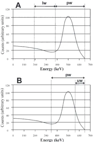
тFigure 2 (A) ٙϯĂ׎̚UE׶LE̶Ҿ΃ܑ͹ਕ඄

(photopeak window) ᄃҲਕ඄ (lower window)ĂR

඄̚೸डְІ۞ּͧ (LE_sc

/UE

)ĂR

ְІ۞ּͧ (LE_unsc

/UE

)ćѩ˟ણᇴߏӀϡቢड໚ٕᕇड

໚дͪ઄វ۞၁រ̚Ր଀Ą၁រ̚Ξͽ៍၅זR_unscд

transaxial FOV̚ೀͼࠎ˘૱ᇴĂ҃R

̙Ӯ̶̹ҶĄд˘ؠ۞ቑಛ̰Ă఺ֱּͧᄃۏវ̂̈൑

ᙯĂЯѩΞͽְА੫၆পؠ۞PETବೡᆇซҖሀᑢĄ൒

҃Ăдྵ̂ۏវ۞ౄᇆ̚ĂR_scдradial͞Шត̼ྵ̂Ăౄ

јۏវγಛ۞೸डְІົజ੼ҤĂЯѩ੫၆ྵ̂۞ۏវ

ֹϡ׽ؠ۞R_scࣃĂּт਒ටౄᇆĂΞਕ̙ዋ༊ĄѩγĂ

Scatter tail

Projection

Object boundary

Counts

Figure 1. Curve fitting method

ϤٺR_scᄃۏវ۞਽ഴܼᇴѣᙯĂѩ͞ڱ၆ܧӮ̹ۏኳϺ

൑ڱઇዋ༊۞ᒣϒĄ

ETM͞ڱ [7] ઄నдߙ࣎ਕณ⼈ࣃͽ˯జ੃ᐂ۞௑

ЪְІΪΒӣϏ೸डְІĄѩ઄నߏЪந۞ĂЯࠎֹϡ

BGO೿វ۞PETବೡጡĂ༊ਕณࠎ511 keVॡĂ׎ਕณྋ

඄ (350-650 keV) ۞ਕณቑಛొ̶ࢦᝑĄ׎̳ёؠཌྷт

˭Ĉ

(2)

Ӏϡд੼ਕ඄ٙפ଀۞ࢍᇴࣃࢷ˯˘ּͧЯ̄ޢĂ ΞՐ଀ৌ၁௑ЪְІ۞࿰ീࣃĂГӀϡ͹ਕ඄ࢍᇴࣃᄃ

࿰ീ۞ৌ၁௑ЪְІᇴ࠹ഴĂགྷ࿅π໣ᕭጡ (smooth fil-

ter) ఍நͽࢫҲϒ୊ဦ (sinogram) ˯۞௚ࢍᄱमĂΞ଀׎

೸ड̶ҶĄ׎̚fࠎּͧЯ̄Ă׎ᄃLORăઍᑭጡϲវ

֎ăਕ඄ቑಛѣᙯĂ҃ᄃड໚̶Ҷ൑ᙯĂЯѩΞְАՐ

଀Ąਕ඄ૄغڱ۞͹ࢋр఍дٺΞͽ҂ᇋֽҋFOVγ۞

೸ड੒ᚥĂтڍֹϡдਕณྋژޘՀр۞೿វ˯Ăּт

LSOĂѩڱᑕྍਕ଀זՀр۞ड़ڍĄਕ඄ૄغڱ͹ࢋ۞

৿ᕇдٺॲፂ˪ڗ (Poisson) ീณ۞ඕڍซҖ೸डࢍზΞ ਕົ͔ˢޝкᗔੈĂ͍׎ߏдજၗౄᇆٕߏࢍᇴࣃѣࢨ

۞ଐڶ˭Ą

୊᎕ഴᖴڱ

࠹၆ٺਕ඄ૄغڱଂᗝγ۞ീณ̚ଯኢ΍೸डྤ

ੈĂ୊᎕ഴᖴڱ (convolution subtraction methodĂᖎჍ

CVS) [2,10-12] ݋઄న೸ड८͕ᄃۏវ̂̈ͽ̈́߿ޘ̶Ҷ

൑ᙯ۞݈೩̝˭Ă೸ड̶ҶΞۡତӀϡ˘࣎ᇾ໤۞͹ਕ

඄Ըᇆྤੈᄃ೸ड८͕ү୊᎕ᖼೱՐ଀Ąѩ͞ڱ੓ܐֹ

ϡٺᒖё2D PET̚Ăдߙ˘࣎পؠ̷ࢬ۞೸डԸᇆ̶Ҷ Ξϡ˘ჯ୊᎕̳ёܑϯĈ

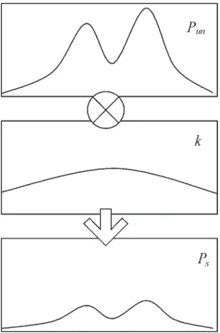
(3)

тFigure 3ٙϯĂ׎̚P_unࠎ͹ࢋְІ۞˘ჯԸᇆćk ࠎᄃ۩ม࠹ᙯ۞೸ड८͕בᇴ (scatter kenel) ΞӀϡٸཉ ቢड໚ٺ઄វ̰̙ТҜཉՐ଀Ąҭߏ̳ё (3) д၁ү˯

ѣ׎ӧᙱĂЯࠎԧࣇ൑ڱפ଀P_un۞ྤੈĄٙضԧࣇΞͽ

ֹϡീณࣃP_obsͽפ΃̳ё (3) ̚۞P_un̪҃Ξჯ޺˘ؠ۞

໤ቁّĄ˘ჯ୊᎕ഴᖴڱ၆ٺ2D PETߏޝ໤ቁ۞ć൒

҃ĂϤٺ3D PET̚FOVγ۞೸डҫ࠹༊۞ּͧ [13]ĂЯ ѩĂࠎ˞҂ᇋFOVγ۞೸ड੒ᚥĂؼҩؠཌྷ΍˟ჯ೸ड ८͕בᇴĂ֭ͷ੫၆Ըᇆྤफ़ેҖ˟ჯ୊᎕т˭Ĉ

(4)

׎̚Ըᇆྤੈᄃ೸ड८͕בᇴؠཌྷࠎradialᄃaxial׌

࣎͞ШĂ ΃ܑ˟ჯ୊᎕ፆү̄Ą˯ࢗ۞˟ჯ୊᎕ഴᖴ ڱͽᝑ΃ڱΐͽࢍზĂ֭ͷӀϡീณࣃP_obs̙ᕝᝑ΃Ҍќ ᑦĂͽҹڇ၁រ̚൑ڱۡତפ଀P_unྤੈ۞યᗟćҌٺ೸

ड८͕ТᇹΞͽӀϡᕇٕቢड໚פᇹ҃଀זĄѩ͞ڱ̏

జᙋ၁дᐝొବೡΞயϠ։р۞ᒣϒड़ڍĄ୊᎕ഴᖴڱ дજၗౄᇆ˯׍ѣ࠹༊۞ᐹ๕ĂЯࠎ׎೸डෞҤૄώ˯

ߏ൑ᗔੈ۞Ăٙͽ̙ົ੒ᚥᗝγ۞ᗔੈҌ೸डᒣϒޢ۞

Figure 2. The dual-energy windows set for (A) the DEW method and (B) the ETM method

Ըᇆྤफ़ĄΩ˘ᐹᕇࠎѩ͞ڱ̙ᅮࢋќะᗝγ۞ਕ඄ྤ

ੈĂЯѩд࿪ཝࢍზ˯Հѣड़தĄ൒҃Ă༊ዎ࿃Հኑᗔ

۞߿ޘ̶ҶĂּт਒ටٕཛొౄᇆॡĂ੓ؕ۞઄నܮ൑

ڱјϲĄࠎ˞Լචѩ˘ዋᑕّ۞৿ᕇĂధкࡁտ࡭˧ٺ ܧ׽ؠّ઄న (non-stationary assumption) ۞ֹϡĂ૟ۏ វ̂̈ă߿ޘ̶Ҷăઍᑭጡϲវ֎ৼˢ҂ᇋĂ൴ण΍Հ ࠎჟቁ۞೸ड८͕ሀݭ [14]ĂЯѩܧ׽ؠّ୊᎕ഴᖴڱ ܮјࠎ˘ໂ׍ሕ˧ͷ΄ˠຏᎸ኷̝ᛉᗟĄ

ሀёૄغڱ

ЯࠎЍ̄дۏኳ̚үϡ۞ۏந፟ט̏జ˞ྋĂԧࣇ ΞᖣϤѩϹ̢үϡ۞পّᄃPETٙפ଀۞ࢦޙᇆညྤ

फ़Ă֭੨Ъᇴࣃ̶ژٕᄋгΙᘲԫఙሀᑢፋ࣎࿅඀ͽࢍ

ზ΍೸ड၆Ըᇆྤफ़۞੒ᚥĂѩᙷݭ۞೸डᒣϒჍࠎሀ ёૄغڱ [15-21]Ą఺ᙷ͞ڱ͹ࢋߏӀϡ͹ਕ඄̚ಏѨ૵

೼ӌ೸डҫፋវ೸डְІ඗̂ొЊ۞পّ (~75%) [14]Ă

֭ Ӏ ϡ ቢ ᎕ ̶ ڱ ͽ ಏ Ѩ ೸ ड ෞ Ҥ ΍ к Ѩ ೸ ड ۞ ณ Ą

Watson [15-17] ያ඾ሀᑢЍ̄۞ዏொĂ൴ण΍ϫ݈జᇃھ

ֹϡ۞Single Scatter Simulation (SSS) ͞ڱĂѩ͞ڱΪ҂

ᇋ׎̚˘̢࣎໑Ѝ̄யϠಏѨ૵೼ӌ೸डĂͽࢍზ΍௑

ЪְІ̚πӮ۞೸ड੒ᚥĄ

SSS

LORֽ̚ҋߙ˘̈೸डડા۞੒ᚥĂ֭૟఺ֱ̈೸डᕇ

ᚥ۞᎕̶҃Ր΍ಏѨ೸ड۞ᓁณĄдЇຍ˘࣎LOR̚ಏ Ѩ೸ड੒ᚥΞͽӀϡ೸ड८͕ᄃ೸डۏវ۞វ᎕̶Ր

଀Ă̳ёт˭Ĉ

(5)

׎̚

R_scatt΃ܑಏѨ೸डְІҫБొ௑ЪְІ۞ּͧ (ኛણ

҂Figure 4ពϯ̝ೀңඕၹ)ćLOR (෍ቢAB) ߏֽҋಏ˘

೸डᕇSٙౄј۞੒ᚥćV_sࠎፋ࣎೸डវ᎕ćn_eࠎ൴डវ

૜ޘ (emitter density)Ăӈࠎࢦޙ۞emission imagećµࠎ

ّ਽ഴܼᇴĂӈࠎࢦޙ۞transmission imagećEࠎࣧؕЍ Figure 3. The scatter distribution (P_s) calculated using a

scatter kernel (k) convoluting with the photopeak data (P_un) in projection space

Figure 4. The scheme of trajectories of scattered photons in the SSS algorithm

̄ਕณ (511 keV)ĂE’ࠎ೸डЍ̄ਕณĂΩ_Sࠎ೸ड֎ޘć

σ

σ

෼ᗓĂઍᑭጡड़த݋ͽ

ε

ε

غڱ൑ڱෞҤ۞̈֎ޘ೸डĄ

SSS͞ڱ۞͹ࢋ৿ᕇࠎӀϡϏགྷ೸डᒣϒ۞ܐؕᇆ

ࢍზֽҋFOVγ۞೸ड੒ᚥĄѣ͛ᚥ၆ѩ೩΍̙Т۞ྋ ՙ͞ڱ [21,22]Ăҭ၆ٺ׍ѣྵ̂axial FOV۞Б֗ౄᇆĂ

SSS͞ڱ۞ֹϡ̪ߏ˘࣎ᅮࢋ޺ᜈᙯڦ۞ᛉᗟĄ

ࢦޙૄغڱ

௚ࢍࢦޙૄغڱ (statistical reconstruction-based scat-

ter correctionĂᖎჍSRBSC) [23]ᄃSSS͞ڱ࠹ТĂ˵Ӏϡ

д௚ࢍёᝑ΃ࢦޙ۞࿅඀̚ĂҲᐛొ̶ќᑦ۞ిޘ੼ٺ

੼ᐛќᑦిޘ [24]ĂЯѩ೸ड̶ҶΞӀϡ݈ೀѨᝑ΃۞

ܐؕᇆညՐ଀Ą׎̳ёт˭Ĉ

(6)

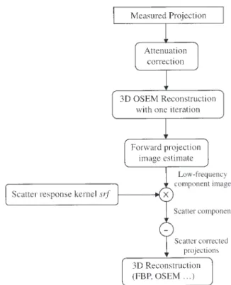
׎̚fࠎৌ၁߿ޘ̶ҶĂΞડ̶ࠎϤҲᐛᇆညf_L׶੼ᐛᇆ ညf_Hٙ௡јĄӀϡ˯ࢗ઄న۞পّĂ૟˘Ѩᝑ΃ޢ۞ᇆ ည (ֹϡOSEMࢦޙڱ) གྷϤϒШԸᇆٙ଀̝ԸᇆྤੈГ ᄃ೸ड८͕בᇴsrfү୊᎕ᖼೱޢĂΞՐ଀೸ड̶ҶĂ׎

ႊზڱтFigure 5ٙϯĄ

SRBSC͞ڱࣘ׍˘ֱ୊᎕ഴᖴڱ۞পّĂТᇹυื

Ր଀ჟቁ۞೸ड८͕ሀݭĄѩ͞ڱ۞ᐹᕇдٺۡତӀϡ

˘Ѩᝑ΃ࢦޙޢᇆည۞Ըᇆྤੈү୊᎕ᖼೱĂ̙ืт

CVS͞ڱᅮࢋкѨᝑ΃఍நĂЯѩࢍზՀ֝ిĄѩ͞ڱ

҃ĂSRBSC͞ڱ۞৿ᕇϺтCVS͞ڱĂ༊ዎ࿃זኑᗔ۞

ۏវॡΞਕ൑ڱ໤ቁ࿰ീ΍೸ड̶ҶĂЯ҃ѣυࢋ൴ण

΍ܧ׽ؠ೸डሀݭĄѩγĂ၆ٺFOVγ೸डҫ˘ؠּͧ

̝͕᝙ବೡᄃБ֗ౄᇆĂSRBSC͞ڱ൑ڱ҂ᇋזFOVγ

ֽ۞೸डְІĂ̪ޞྋՙĄ

डՁܡጿ྅ཉڱ

डՁܡጿ྅ཉڱ (beam stopper device methodĂᖎჍ

BS) [25]Ăࠎԧࣇ၁រވܕೀѐ۞ࡁտјڍĄܡጿጡߏӀ

઄న୧І˭Ăܡጿጡົͽ˘ؠ۞ּͧ਽ഴ͹ࢋЍ̄ĄӀ ϡѣ൑ٸཉѩडՁܡጿ྅ཉ۞मளĂ೸ड۞ณٕߏ೸ड

̶தΞͽۡତଂజܡጿ۞LOR̚Ր଀Ă̳ёт˭Ĉ

(7)

׎̚SăP̶Ҿܑϯࣧؕੈཱི̚೸डొЊᄃ͹ࢋडՁొ

ЊĂC_Rܑϯ̙ӣडՁܡጿ྅ཉ۞ౄᇆ̚LOR (t,

θ ) ˯۞ࢍ

ᇴࣃĂC_BܑϯӣडՁܡጿ྅ཉ۞ౄᇆ̚LOR (t,

θ ) ˯۞ࢍ

ᇴࣃĄӀϡѣ൑ܡጿ྅ཉ۞۩ঈବೡ (air scan) ၁រĂӈ Ξീ଀ࡍ౅Ѻ̶ͧTࣃĂᖣѩࢍზ΍˯̳ࢗё̚ᑫ๴྅

ཉפᇹᕇti˯۞೸डྤੈĄ઄న೸ड۞۩ม̶Ҷߏቤၙត

̼۞בᇴĂԧࣇΞͽӀϡcublic splinḛ೧ڱՐ଀дϒ୊

ဦ̚ፋ࣎೸ड۞̶ҶтFigure 6 (B) ٙϯĄ

Figure 5. The flow chart illustrating the general principle of the SRBSC algorithm

BS

FOVγ۞೸ड੒ᚥĂ၆ٺྵኑᗔ۞ۏវᄃ̙Ӯ̹۞߿ޘ

̶ҶĂBS͞ڱౌΞ྿ז։р۞ᒣϒड़ڍĄBS͞ڱ۞͹ࢋ

৿ᕇࠎडՁܡጿ྅ཉώ֗ϺΞਕౄј೸डְІ۞਽ഴĂ ซ҃ౄј೸ड௑ЪְІ۞੼ҤĂ̙࿅఺࣎৿ᕇΞགྷϤ౵

ָ̼डՁܡጿጡ۞̂̈ᄃᇴϫΐͽҹڇĄԧࣇགྷϤԼត

̙ТܡጿጡΗशᄃᇴϫ۞௡ЪĂ൴னܡጿጡ۞Ηश෸

̈Ă೸डᒣϒ۞ඕڍ෸рĂ੫၆۱ొ۞ˠݭ઄វ҃֏Ă

16࣎Ηश3̳ᗃ۞ܡጿጡΞͽயϠ౵໤ቁ۞ᒣϒඕڍĄѦ

੅ኢ

ტЪЧ჌೸डᒣϒڱ۞ᐹКΞͽ൴னĂ೸डᒣϒٙ

ਕ྿ז۞໤ቁޘᄃ׎ᑕϡ૟פՙٺޞീۏវ۞̂̈ᄃ૜

ޘăۏវ̰߿ޘ̶Ҷăઍᑭጡ۞ԛёăਕ඄ቑಛͽ̈́פ ᇹሀё҃ѣ̙Т۞ܑனĄдཝొବೡ̚ĂϤٺᐝొ۞਽

ഴܼᇴត̼࠹၆ྵ̈ᄃٙҫFOVቑಛྵ̈۞পّĂֹ଀

೸डᒣϒྵࠎटٽĂٙѣᒣϒڱٙ଀ז۞ඕڍ˵ྵࠎ໤

ቁĄҭߏ၆ٺ਒ొᄃཛొବೡ҃֏Ăੵ˞ТҜ৵̶Ҷ̙

Ӯ̹γĂ௡ᖐ૜ޘ۞मளĂ˵ౄј೸डᒣϒ۞ӧᙱĂ఺

͞ࢬሀёૄغڱ̏జរᙋਕѣड़۞ொੵ೸डѳߖĂҭߏ ҡᐌֽ҃۞̂ณྻზ˵ឰ఺ֱӀϡᝑ΃ёႊზڱ۞ᓜԖ ᑕϡ΍ன஬ᐚĄ

д3Dפᇹሀё̚ĂFOVγֽ۞೸ड੒ᚥΞ྿זБొ

೸डְІ۞50% [13]Ăѩॡᑕϡ̰೧૜Ъڱᄃਕ඄ૄغ ڱΞѣड़ொੵкѨ೸ड۞੒ᚥĂ൒҃ૄٺᗝγਕ඄۞ྤ

फ़఼૱ົҡᐌ඾ᗝγ۞ᗔੈĂ఺ᙷ͞ڱྵ̙ዋЪᑕϡд Figure 6. (A) For each projection angle, the primary events

are blocked at several radial bins. (B) The scatter distribution (dotted line) is interpolated based on the scatter components (solid arrow) estimated at those blocked bins.

Figure 7. The reconstructed images of the Zubal phantom. (A) The reference image used as input to the simulator, (B) uncor- rected image, and (C) image corrected by the BS method

જၗౄᇆ˯ĄBS͞ڱტЪ˞˯ࢗ۞ᐹᕇĂੵ˞Ξͽᑕϡ ٺྵ̂ͷྵኑᗔ۞ۏវౄᇆ˯Ă၆ٺFOVγֽ۞೸डѳ ߖ˵ΞͽΐͽொੵĂЯѩĂ೩ֻ˞໤ቁ೸डᒣϒ۞Ξਕ

ّĄ

ܕѐֽ੫၆ϒ̄࿪ཝᕝᆸؠณ۞υᅮّĂቁ၁͔൴

˞˘ֱ੅ኢ [26]ĂӀϡߴ-18ซҖ඗၆ؠณੵ˞צࢨٺొ

Њវ᎕ (partial volume) યᗟͽγĂՀᅮࢋࢬ၆ኑᗔ۞ᒣ ϒՎូĂֹ଀඗၆ؠณдᓜԖ˯۞ᑕϡ̙ٽଯҖĂϫ݈

кΗ˵Ϊϡٺߴ-18-FDGᇾ໤ӛќࣃ (standard uptake

value)

̙֭ົᇆᜩᒛা۞ડ̶ᄃҿؠ [27]Ăҭߏ၆ٺ˘ֱপঅ ८჌۞ᑕϡᄃߴ-18-FDG۞࠹၆ؠณ (ᇆညᇴࣃϒͧٺߙ

˘តᇴ)ĂᓜԖ˯ᔘߏ׍ѣ˘ؠ۞ຍཌྷхдĂּтĈֹϡ Ḳ-86 (⁸⁶

Y) ۞඗၆ؠณͽ໤ቁෞҤḲ-86 (

Y) ۞ТҜ৵ڼ

۞ĄҌٺ೸डᒣϒ၆ٺཚሳઍീத۞೩̿ߏӎ׍ѣड़ ڍĂϫ݈إϏ଀ז˘࡭۞ඕኢĂ੫၆̈ٺ2̶̳۞۱ొᒛ

াĂࡁտඕڍᄮࠎ೸डᒣϒᄃ਽ഴᒣϒΞͽᆧΐઍീத

[29]Ăҭߏ၆ٺྵ̂ཚሳઍീத۞Լត݋̙׍௚ࢍຍ

ඕኢ

ͧྵЧ჌೸डᒣϒ͞ڱĂΞͽ࠻΍఺̱ᙷ۞ԫఙౌ

Чѣ׎ᐹ৿ᕇĂ఺˵ពϯ΍೸डᒣϒ۞ࢦࢋّᄃ઼ᅫม д೸डᒣϒᅳા˯ٙઇ۞Ӆ˧ĄტЪ˯ࢗᒣϒ͞ڱ̝ᐹ Кᕇâ࣎јሢ۞೸डᒣϒڱᑕྍ׍ѣ˭Е۞পّĈ (1) ਕТॡ఍நFOV̰ᄃγயϠ۞೸डְІć(2) ਕۡତᒣϒ ಏѨ೸डᄃкࢦ೸ड۞੒ᚥć(3) ਕ҂ᇋ̈֎ޘ۞೸डְ

Іć(4) ਕ଀ז໤ቁ۞೸ड̶Ҷᄃ೸ड̶த̶Ҷć(5) ਕ

҂ᇋޞീۏវᄃPETବೡᆇ۞পّć(6) ਕԣిซҖᒣϒ үຽĄ

ϫ݈إ൑Ԇ࡚۞೸डᒣϒڱĂ҃Տ˘჌͞ڱ˵ౌื

ࢋֶፂߙ჌পؠ۞઄న୧І˭̖ਕ྿ז໤ቁ۞ᒣϒඕ ڍĂЯѩ࠹ᙯ۞ࡁտ̪ืᚶᜈซҖĄ೸डᒣϒϏֽ൴ण ᔌ๕Ξ̶ࠎᇴ࣎͞ШĂඕЪ̙Тᙷݭ۞ᒣϒڱၟܜྃ

ൺĂͽՀჟቁ۞ෞҤ೸ड۞̶Ҷߏ˘࣎ΞҖ۞͞ڱĂּ

тĈඕЪBS͞ڱᄃਕ඄ૄغڱͽࢍზ೸ड̶த۞̶ҶĄ ᐌ඾࿪ཝ۞ԣి൴णĂԧࣇΞͽޙၹՀჟ૜۞ણᇴሀݭ

ͽ఍ந೸ड۞યᗟĂּтĈܧ׽ؠ୊᎕ഴᖴڱᄃࢦޙૄ

غڱ۞൴णᄃॲፂࢦޙᇆညࠎૄᖂٙ൴ण΍۞ሀёૄغ ڱĄѩγĂӀϡᕍะ࿪ཝ۞πҖ఍நਕ˧ٺᄋгΙᘲ۞

ӈॡሀᑢ˯Ă૟಼̂۞ᒺൺྻზॡมĂ࠹ܫ̙˳۞૟

ֽĂ੫၆࣎ҾঽˠซҖӈॡᄋгΙᘲሀᑢͽՐ଀೸ड̶

ҶĂΞۡତᑕϡٺᓜԖ۞ˬჯϒ̄࿪ཝᕝᆸౄᇆ˯Ą

ણ҂͛ᚥ

1. Johns HE, Cunningham JR eds. The Physics of Radiology. 4th ed. Springfield, USA: Charles C.

Thomas; 1983:176-179.

2. Bailey DL, Meikle SR. A convolution-subtraction scatter correction method for 3D PET. Phys Med Biol 1994;39:411-424.

3. Cherry SR, Meikle SR, Hoffman EJ. Correction and characterization of scattered events in three-dimensional PET using scanners with retractable septa. J Nucl Med 1993;34:671-678.

4. Cherry SR, Huang SC. Effects of scatter on model para- meter estimates in 3D PET studies of the human brain.

IEEE Trans Nucl Sci 1995;42:1174-1179.

5. Grootoonk S, Spinks TJ, Jones T, Michel C, Bol A.

Correction for scatter using a dual energy window tech- nique with a tomograph operating without septa. IEEE Med Imag Conf Rec 1991;3:1569-1573.

6. Grootoonk S, Spinks TJ, Sashin D, Spyrou NM, Jones T.

Correction for scatter in 3D brain PET using a dual ener- gy window method. Phys Med Biol 1996;41:2757-2774.

7. Bendriem B, Trebossen R, Frouin V, Syrota A. A PET scatter correction using simultaneous acquisitions with low and high energy thresholds. IEEE Med Imag Conf Rec 1993;3:1779-1783.

8. Shao L, Freifelder R, Karp JS. Triple energy window scatter correction method for PET. IEEE Trans Med Imag 1994;13:641-648.

9. Jaszczak RJ, Greer KL, Floyd CE Jr, Harris CC, Coleman RE. Improved SPECT quantification using compensation for scattered photons. J Nucl Med 1984;25:893-900.

10. McKee BTA, Gurvey AT, Harvey PJ, Howse DC. A

deconvolution scatter correction for a 3D PET system.

IEEE Trans Med Imag 1992;11:560-569.

11. Shao L, Karp JS. Cross-plane scattering correction- point source deconvolution in PET. IEEE Trans Med Imag 1991;10:234-239.

12. Bentourkia M, Msaki P, Cadorette J, Lecompte R.

Assessment of scatter components in high-resolution PET: correction by nonstationary convolution subtrac- tion. J Nucl Med 1995;36:121-130.

13. Adam LE, Karp JS, Brix G. Investigation of scattered radiation in 3D whole-body positron emission tomogra- phy using Monte Carlo simulations. Phys Med Biol 1999;44:2879-2895.

14. Zaidi H, Koral KF. Scatter modelling and compensation in emission tomography. Eur J Nucl Med Mol Imag 2004;31:761-782.

15. Watson CC, Newport D, Casey ME, deKemp RA, Beanlands RS, Schniand M. Evaluation of simulation- based scatter correction for 3-D PET cardiac imaging.

IEEE Trans Nucl Sci 1997;44:90-97.

16. Watson CC. New, faster, image-based scatter correction for 3D PET. IEEE Trans Nucl Sci 2000;47:1587-1594.

17. Watson CC, D Newport, Casey ME. A single scatter sim- ulation technique for scatter correction in 3D PET. In:

Grangeat P, Amans JL, eds. Three-Dimensional Image Reconstruction in Radiology and Nuclear Medicine.

Dordrecht: Kluwer Academic; 1996:255-268.

18. Ollinger JM. Model-based scatter correction for fully 3D PET. Phys Med Biol 1996;41:153-176.

19. Levin CS, Dahlbom M, Hoffman EJ. A Monte Carlo cor- rection for the effect of Compton scattering on 3-D PET imaging. IEEE Trans Nucl Sci 1995;42:1181-1185.

20. Wollenweber SD. Parameterization of a model-based 3- D PET scatter correction. IEEE Trans Nucl Sci 2002;49:722-727.

21. Werling A, Bublitz O, Doll J, Adam LE, Brix G. Fast implementation of the single scatter simulation algorithm and its use in iterative reconstruction of 3D PET data.

Phys Med Biol 2002;47:2947-2960.

22. Ferreira NC, Trebossen R, Lartizien C, Brulon V, Merceron P, Bendriem B. A hybrid scatter correction for 3D PET based on an estimation of the distribution of unscattered coincidences: implementation on the ECAT EXACT HR+. Phys Med Biol 2002;47:1555-1571.

23. Zaidi H. Reconstruction-based estimation of the scatter component in positron emission tomography. Ann Nucl Med Sci 2001;14:161-171.

24. Pan TS, Yagle AE. Numerical study of multigrid imple- mentations of some iterative image reconstruction algo- rithms. IEEE Trans Med Imag 1991;10:572-588.

25. Chuang KS, Wu J, Jan ML, Chen S, Hsu CH. Novel scatter correction for three-dimensional positron emis- sion tomography by use of a beam stopper device. Nucl Instr and Meth A 2005 (in press).

26. Marsden PK. Quantification in PET: what is it? Can we do it? Do we need it? Nucl Med Commun 2004;25:635- 636.

27. Strother SC, Liow JS, Moeller JR, Sidtis JJ, Dhawan VJ, Rottenberg DA. Absolute quantitation in neurological PET: do we need it? J Cereb Blood Flow Metab 1991;11:A3-A16.

28. Pentlow KS, Finn RD, Larson SM, Erdi YE, Beattie BJ, Humm JL. Quantitative imaging of yttrium-86 with PET.

The occurrence and correction of anomalous apparent activity in high density regions. Clin Positron Imag 2000;3:85-90.

29. Zhang H, Tian M, Oriuchi N, Higuchi T, Tanada S, Endo K. Detection of lung cancer with positron coincidence gamma camera using fluorodeoxyglucose in comparison with dedicated PET. Eur J Radiol 2003;47:199-205.

30. Montandon ML, Slosman DO, Zaidi H. Assessment of

the impact of model-based scatter correction on

F-FDG

3D brain PET in healthy subjects using statistical para-

metric mapping. Neuroimage 2003;20:1848-1856.

A Review of Scatter Correction Methods for Three-Dimensional Positron Emission Tomography

Jay Wu

, Hsing-Hon Lin

, Keh-Shih Chuang

1

Department of Radiological Technology, Central Taiwan University of Science and Technology, Taichung, Taiwan

2

Department of Nuclear Science, National Tsing-Hua University, Hsinchu, Taiwan

Received 8/23/2005; revised 9/27/2005; accepted 9/28/2005.

For correspondence or reprints contact: Jay Wu, Ph.D., Department of Radiological Technology, Central Taiwan University of Science and Technology, 11 Pu-Tzu Lane, Pei-tun District, Taichung 406, Taiwan. Tel: (886)-928246662, Fax: (886)3-4891792, E-mail: [email protected]

Positron emission tomography (PET) offers the possibility of quantitative assessment of tracer concentration in vivo.

Fully 3D PET can achieve higher system sensitivity of coincidence events than the 2D mode, but the absence of inter-slice septa inevitably leads to increased scattered events. The scattered events can contribute as much as 50% of the total detected events. Therefore, accurate correction for the scatter component is necessary for mean- ingful quantitative image analysis and tracer kinetic modeling. A number of scatter correction methods have been proposed and successfully implemented for 3D PET. In this article, we comprehensively reviewed five scatter cor- rection approaches, including curve fitting method, energy-based method, convolution subtraction method, model- based method, reconstruction-based method, and our newly developed beam stopper approach.

Key words: 3D PET, scatter correction, beam stopper device

Ann Nucl Med Sci 2005;18:225-233