國立臺灣大學工程學院化學工程學系 碩士論文
Department of Chemical Engineering College of Engineering
National Taiwan University Master Thesis
內隔壁式蒸餾塔之動態與控制
Dynamics and Control of Divided Wall Columns
趙傳真 Chuan-Chen Chao
指導教授: 吳哲夫 博士 Advisor: Jeffrey D. Ward, Ph.D.
中華民國 100 年 7 月
July, 2011
誌謝
在此,由衷的感謝吾師 吳哲夫教授,在為期不長的兩年時間裡敎會了我很多的東 西,不只在研究學習方面,做人處事方面也是我的學習標的,此等用心,著實難得可貴。
這種亦師亦友的的情誼將會是難以忘懷的一個回憶。感謝陳誠亮教授、錢義隆教授與黃 孝平教授給予我的諸多指導與建議。
在離鄉兩年的學習間,也要感謝我的家人對我的支持,你們的鼓勵,是我堅持下去 的動力,我最最親愛的家人,沒有你們,這份學業很難完成,爸、媽、弟、雯,謝謝。
接者要感謝同窗: 郁迪,博士班加油囉;宗翰,別忘了清粥小菜、復興南豆漿以及
頂樓美好的時光;哲維,教我彈吉他吧QQ;均諺,六年的時光轉眼即逝,我們進化了;
孟達,俄羅斯方塊魔人,不要再色下去了;育賢,你很愛生氣耶,魔獸打輸我別難過,
再練練就好;鎮宇,喔醬、這樣尼。
最後感謝學長姊們 ( 豪業、建凱、乾元、義章、士暐、瑞元、志曜、愷悌、玉龍、
雅玲、Anton、佳紘、國超、昱峰、明璟、媛翎、詩雯、Anggi ) 與學弟們 ( 恒嘉、紹 群、偉倫、子軒、桐霖、旻澤、滕允 ),謝謝。
摘要
相較於傳統的蒸餾序列,內隔壁式蒸餾塔 (DWC) 是一種在分離多成分混合物時,
可以節省更多的能量與設備成本的前瞻性設計。然而,內隔壁式蒸餾塔在設計上也較為 困難,因為較傳統序列擁有更多的設計自由度。約莫五十年前,內隔壁式蒸餾塔的設計 方法被提出討論,許多論文討論穩態設計問題,並提出啟發式和嚴謹的設計優化方法。
但是,內隔壁式蒸餾塔的控制相對的得到較少的關注。此研究主要是針對內隔壁式蒸餾 塔分離理想系統的可控性進行調查。對於不同類型的內隔壁式蒸餾塔、不同相對揮發度 的分離指標、不同的進料條件,進行可控性的分析。並對於不同的控制策略,採用線性 分析工具,相對增益陣列 (RGA) 和條件數 (CN) 進行分析。論文中為符合實際工廠使 用的控制策略,利用進料擾動從動態上測試其排除干擾的能力。最後,從控制的角度提 出一選擇何種類型內隔壁式蒸餾塔之指導方針。 從控制的觀點發現,當進料含有較多 輕成分時建議使用上隔板式蒸餾塔;當進料含有較多中間成分時建議使用下隔板式蒸餾 塔;當進料含有較多重成分時建議使用上隔板式蒸餾塔。
關鍵字: 內隔壁式蒸餾,控制,相對增益陣列
Abstract
The divided-wall column system is a promising energy saving alternative for separating multi-component mixtures compared with traditional distillation columns. However the design of DWCs is more difficult because there are more degrees of freedom. The control of the DWC have received much less attention. In this work, the controllability of a divided wall column for separating ideal system were investigated. The main objective of this work is to study the divided-wall column (DWC) controllability. A controllability analysis of the ideal system is done for the separation of different types of DWC, different ease separation index (ESI) and different feed condition. Different control structures are compared using linear analysis tools, relative gain array (RGA) and condition number (CN). Disturbances in feed fowrate and feed composition are used to demonstrate the effectiveness of the proposed control structure. Finally, a guideline for the selection of the divided-wall column is proposed.
Based on control considerations for different feed conditions, it is found that: If there is more lightest component in the feed, DWCU is preferred. If there is more middle component in the feed, DWCL is preferred. If there is more heaviest component in the feed, DWCU is
Table of Contents
誌謝 ... i
摘要 ... iii
Abstract ... v
Table of Contents ... vii
List of Figures ... xi
List of Tables ... xix
1 Introduction ... 1
1.1 Preface ... 1
1.2 Introduction for DWCs ... 4
1.2.1 DWCL ... 4
1.2.2 DWCU ... 5
1.4 Motivation ... 13
1.5 Thesis organization... 14
2 Steady-State Analysis ... 15
2.1 Thermodynamic properties ... 15
2.2 Shortcut method ... 18
2.3 Analysis method ... 26
2.3.1 Relative Gain Array ... 26
2.3.2 Condition Number ... 29
2.4 Results ... 30
2.4.1 DWCL ... 31
2.4.2 DWCU ... 44
2.4.3 DWCM ... 45
2.5 Summary ... 58
3 Dynamic Analysis ... 63
3.1 Dynamic simulation ... 63
3.2 Analysis method ... 65
3.2.1 Integral Error Criteria ... 65
3.3 Results of feed flowrate disturbance ... 66
3.3.1 DWCL ... 66
3.3.2 DWCU ... 83
3.3.3 DWCM ... 97
3.4 Results of feed composition disturbance ... 116
3.5 Summary ... 118
4 Conclusion ... 123
Appendix A ... 129
Reference ... 135
List of Figures
Fig. 1.1-1 Direct sequence (DS). ... 1
Fig. 1.1-2 B composition profile in the first column and remixing phenomenon. ... 2
Fig. 1.2-1 The evolution of DWCL ... 4
Fig. 1.2-2 The evolution of DWCU. ... 6
Fig. 1.2-3 The evolution of DWCM. ... 7
Fig. 2.2-1 Shortcut design procedure for DWCL ... 19
Fig. 2.2-2 Shortcut design procedure for DWCU ... 19
Fig. 2.2-3 Shortcut design procedure for DWCM. ... 20
Fig. 2.2-4 The configuration of DWCL ... 22
Fig. 2.2-5 The configuration of DWCU ... 22
Fig. 2.2-6 The configuration of DWCM ... 25
Fig. 2.5-1 Results of RGA and CN for DWCL of ESI>1. ... 58
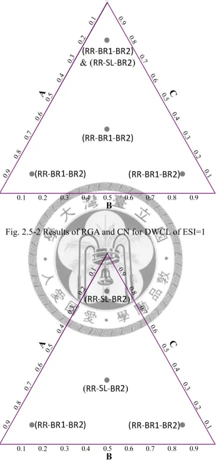
Fig. 2.5-2 Results of RGA and CN for DWCL of ESI=1. ... 59
Fig. 2.5-3 Results of RGA and CN for DWCL of ESI<1. ... 59
Fig. 3.3-1 Control Structure RR-BR1-BR2 for DWCL. ... 67
Fig. 3.3-2 Control Structure SL-BR1-BR2 for DWCL. ... 68
Fig. 3.3-3 Control Structure RR-SL-BR2 for DWCL. ... 69
Fig. 3.3-4 Control Structure RR-BR1-SL for DWCL. ... 70
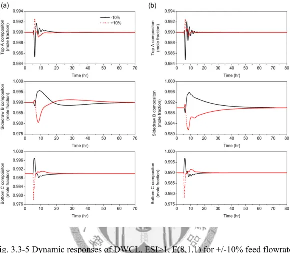
Fig. 3.3-5 Dynamic responses of DWCL, ESI>1, F(8,1,1) for +/-10% feed flowrate disturbances. (a) RR-BR1-BR2 (b) RR-SL-BR2 ... 71
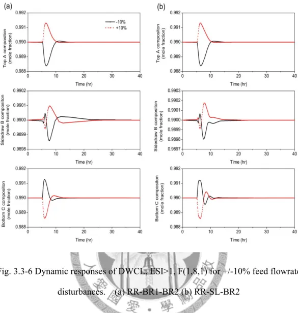
Fig. 3.3-6 Dynamic responses of DWCL, ESI>1, F(1,8,1) for +/-10% feed flowrate disturbances. (a) RR-BR1-BR2 (b) RR-SL-BR2 ... 72
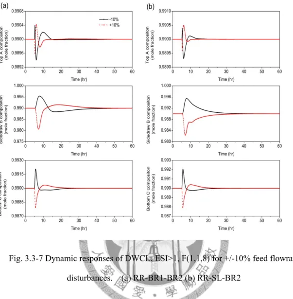
Fig. 3.3-7 Dynamic responses of DWCL, ESI>1, F(1,1,8) for +/-10% feed flowrate disturbances. (a) RR-BR1-BR2 (b) RR-SL-BR2 ... 73
Fig. 3.3-8 Dynamic responses of DWCL, ESI>1, F(3,3,3) for +/-10% feed flowrate disturbances. (a) RR-BR1-BR2 (b) RR-SL-BR2 ... 74
Fig. 3.3-9 Dynamic responses of DWCL, ESI=1, F(8,1,1) for +/-10% feed flowrate disturbances. (a) RR-BR1-BR2 (b) RR-SL-BR2 ... 75
Fig. 3.3-10 Dynamic responses of DWCL, ESI=1, F(1,8,1) for +/-10% feed flowrate disturbances. (a) RR-BR1-BR2 (b) RR-SL-BR2 ... 76
Fig. 3.3-11 Dynamic responses of DWCL, ESI=1, F(1,1,8) for +/-10% feed flowrate disturbances. (a) RR-BR1-BR2 (b) RR-SL-BR2 ... 77
Fig. 3.3-12 Dynamic responses of DWCL, ESI=1, F(3,3,3) for +/-10% feed flowrate disturbances. (a) RR-BR1-BR2 (b) RR-SL-BR2 ... 78 Fig. 3.3-13 Dynamic responses of DWCL, ESI<1, F(8,1,1) for +/-10% feed flowrate
disturbances. (a) RR-BR1-BR2 (b) RR-SL-BR2 ... 79 Fig. 3.3-14 Dynamic responses of DWCL, ESI<1, F(1,8,1) for +/-10% feed flowrate
disturbances. (a) RR-BR1-BR2 (b) RR-SL-BR2 ... 80 Fig. 3.3-15 Dynamic responses of DWCL, ESI<1, F(1,1,8) for +/-10% feed flowrate
disturbances. (a) RR-BR1-BR2 (b) RR-SL-BR2 ... 81 Fig. 3.3-16 Dynamic responses of DWCL, ESI<1, F(3,3,3) for +/-10% feed flowrate
disturbances. (a) RR-BR1-BR2 (b) RR-SL-BR2 ... 82 Fig. 3.3-17 Control Structure RR1-RR2-BR for DWCU. ... 84 Fig. 3.3-18 Dynamic responses of DWCU, ESI>1, F(8,1,1) for +/-10% feed flowrate
disturbances. RR1-RR2-BR ... 85 Fig. 3.3-19 Dynamic responses of DWCU, ESI>1, F(1,8,1) for +/-10% feed flowrate
disturbances. RR1-RR2-BR ... 86 Fig. 3.3-20 Dynamic responses of DWCU, ESI>1, F(1,1,8) for +/-10% feed flowrate
disturbances. RR1-RR2-BR ... 88 Fig. 3.3-22 Dynamic responses of DWCU, ESI=1, F(8,1,1) for +/-10% feed flowrate
disturbances. RR1-RR2-BR ... 89 Fig. 3.3-23 Dynamic responses of DWCU, ESI=1, F(1,8,1) for +/-10% feed flowrate
disturbances. RR1-RR2-BR ... 90 Fig. 3.3-24 Dynamic responses of DWCU, ESI=1, F(1,1,8) for +/-10% feed flowrate
disturbances. RR1-RR2-BR ... 91 Fig. 3.3-25 Dynamic responses of DWCU, ESI=1, F(3,3,3) for +/-10% feed flowrate
disturbances. RR1-RR2-BR ... 92 Fig. 3.3-26 Dynamic responses of DWCU, ESI<1, F(8,1,1) for +/-10% feed flowrate
disturbances. RR1-RR2-BR ... 93 Fig. 3.3-27 Dynamic responses of DWCU, ESI<1, F(1,8,1) for +/-10% feed flowrate
disturbances. RR1-RR2-BR ... 94 Fig. 3.3-28 Dynamic responses of DWCU, ESI<1, F(1,1,8) for +/-10% feed flowrate
disturbances. RR1-RR2-BR ... 95 Fig. 3.3-29 Dynamic responses of DWCU, ESI<1, F(3,3,3) for +/-10% feed flowrate
disturbances. RR1-RR2-BR ... 96 Fig. 3.3-30 Control Structure RR-S-BR for DWCM. ... 98
Fig. 3.3-31 Control Structure S-S-BR for DWCM. ... 99
Fig. 3.3-32 Control Structure S-SL-BR for DWCM. ... 100
Fig. 3.3-33 Control Structure BR-SL-S for DWCM. ... 101
Fig. 3.3-34 Control Structure RR-SL-BR for DWCM. ... 102
Fig. 3.3-35 Control Structure RR-S-SL for DWCM. ... 103
Fig. 3.3-36 Control Structure RR-SL-S for DWCM. ... 104
Fig. 3.3-37 Dynamic responses of DWCM, ESI>1, F(8,1,1) for +/-10% feed flowrate disturbances. S-SL-BR ... 104
Fig. 3.3-38 Dynamic responses of DWCM, ESI>1, F(1,8,1) for +/-10% feed flowrate disturbances. RR-S-BR ... 105
Fig. 3.3-39 Dynamic responses of DWCM, ESI>1, F(1,1,8) for +/-10% feed flowrate disturbances. (a) S-SL-BR (b) RR-SL-S ... 106
Fig. 3.3-40 Dynamic responses of DWCM, ESI>1, F(3,3,3) for +/-10% feed flowrate disturbances. S-RR-BR ... 107
Fig. 3.3-41 Dynamic responses of DWCM, ESI=1, F(8,1,1) for +/-10% feed flowrate disturbances. S-SL-BR ... 108
Fig. 3.3-43 Dynamic responses of DWCM, ESI=1, F(1,1,8) for +/-10% feed flowrate disturbances. RR-SL-S ... 110 Fig. 3.3-44 Dynamic responses of DWCM, ESI=1, F(3,3,3) for +/-10% feed flowrate
disturbances. S-SL-BR ... 111 Fig. 3.3-45 Dynamic responses of DWCM, ESI<1, F(8,1,1) for +/-10% feed flowrate
disturbances. S-SL-BR ... 112 Fig. 3.3-46 Dynamic responses of DWCM, ESI<1, F(1,8,1) for +/-10% feed flowrate
disturbances. (a) RR-S-BR (b) RR-S-SL ... 113 Fig. 3.3-47 Dynamic responses of DWCM, ESI<1, F(1,1,8) for +/-10% feed flowrate
disturbances. RR-SL-S ... 114 Fig. 3.3-48 Dynamic responses of DWCM, ESI<1, F(3,3,3) for +/-10% feed flowrate
disturbances. S-SL-BR ... 115 Fig. 3.4-1 Dynamic responses of DWCL, ESI=1, F(3,3,3) for +/-10% feed composition
disturbances. RR-BR1-BR2 ... 116 Fig. 3.4-2 Dynamic responses of DWCU, ESI=1, F(3,3,3) for +/-10% feed composition
disturbances. RR1-RR2-BR ... 117 Fig. 3.4-3 Dynamic responses of DWCU, ESI=1, F(3,3,3) for +/-10% feed composition
disturbances. RR-SL-BR ... 117
Fig. 3.5-1 Results of dynamic response for DWCL of ESI>1 ... 118
Fig. 3.5-2 Results of dynamic response for DWCL of ESI=1 ... 119
Fig. 3.5-3 Results of dynamic response for DWCL of ESI<1 ... 119
Fig. 3.5-4 Results of dynamic response for DWCM of ESI>1 ... 120
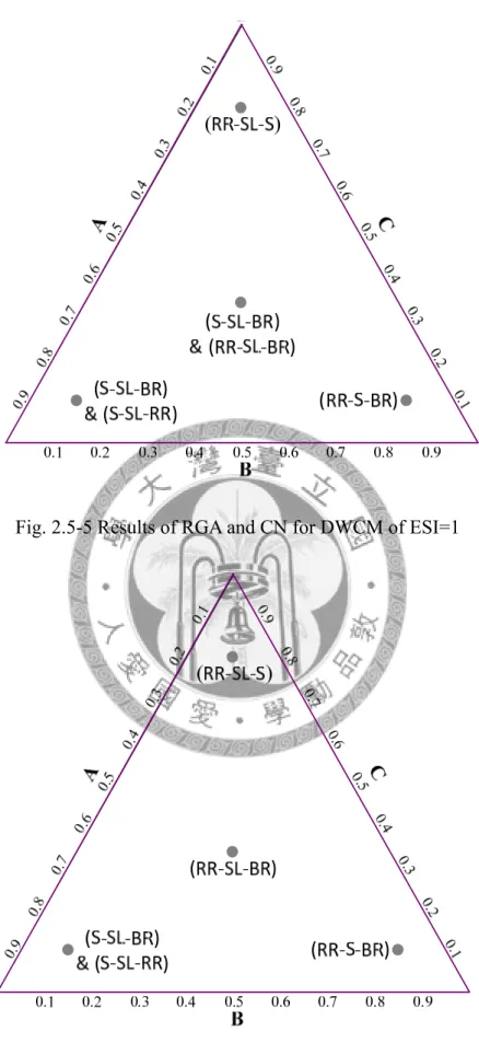
Fig. 3.5-5 Results of dynamic response for DWCM of ESI=1 ... 121
Fig. 3.5-6 Results of dynamic response for DWCM of ESI<1 ... 121
List of Tables
Table 2.1-1 Thermodynamic parameters for ideal system ( ESI>1 ) ... 16
Table 2.1-2 Thermodynamic parameters for ideal system ( ESI=1 ) ... 16
Table 2.1-3 Thermodynamic parameters for ideal system ( ESI<1 ) ... 17
Table 2.2-1 Tray number of DWCL ... 21
Table 2.2-2 Tray number of DWCU ... 23
Table 2.2-3 Tray number of DWCM ... 24
Table 2.4-1 RGA and CN analysis for DWCL, ESI>1, F(8,1,1) ... 32
Table 2.4-2 RGA and CN analysis for DWCL, ESI>1, F(1,8,1) ... 33
Table 2.4-3 RGA and CN analysis for DWCL, ESI>1, F(1,1,8) ... 34
Table 2.4-4 RGA and CN analysis for DWCL, ESI>1, F(3,3,3) ... 35
Table 2.4-5 RGA and CN analysis for DWCL, ESI=1, F(8,1,1) ... 36
Table 2.4-6 RGA and CN analysis for DWCL, ESI=1, F(1,8,1) ... 37
Table 2.4-7 RGA and CN analysis for DWCL, ESI=1, F(1,1,8) ... 38
Table 2.4-8 RGA and CN analysis for DWCL, ESI=1, F(3,3,3) ... 39
Table 2.4-12 RGA and CN analysis for DWCL, ESI<1, F(3,3,3) ... 43
Table 2.4-13 RGA and CN analysis for DWCM, ESI>1, F(8,1,1) ... 46
Table 2.4-14 RGA and CN analysis for DWCM, ESI>1, F(1,8,1) ... 47
Table 2.4-15 RGA and CN analysis for DWCM, ESI>1, F(1,1,8) ... 48
Table 2.4-16 RGA and CN analysis for DWCM, ESI>1, F(3,3,3) ... 49
Table 2.4-17 RGA and CN analysis for DWCM, ESI=1, F(8,1,1) ... 50
Table 2.4-18 RGA and CN analysis for DWCM, ESI=1, F(1,8,1) ... 51
Table 2.4-19 RGA and CN analysis for DWCM, ESI=1, F(1,1,8) ... 52
Table 2.4-20 RGA and CN analysis for DWCM, ESI=1, F(3,3,3) ... 53
Table 2.4-21 RGA and CN analysis for DWCM, ESI<1, F(8,1,1) ... 54
Table 2.4-22 RGA and CN analysis for DWCM, ESI<1, F(1,8,1) ... 55
Table 2.4-23 RGA and CN analysis for DWCM, ESI<1, F(1,1,8) ... 56
Table 2.4-24 RGA and CN analysis for DWCM, ESI<1, F(3,3,3) ... 57 Table 3.3-1 IAE and ITAE value of DWCL, ESI>1, F(8,1,1) for different control structures 71 Table 3.3-2 IAE and ITAE value of DWCL, ESI>1, F(1,8,1) for different control structures 72 Table 3.3-3 IAE and ITAE value of DWCL, ESI>1, F(1,1,8) for different control structures 73 Table 3.3-4 IAE and ITAE value of DWCL, ESI>1, F(3,3,3) for different control structures 74 Table 3.3-5 IAE and ITAE value of DWCL, ESI=1, F(8,1,1) for different control structures 75
Table 3.3-6 IAE and ITAE value of DWCL, ESI=1, F(1,8,1) for different control structures 76 Table 3.3-7 IAE and ITAE value of DWCL, ESI=1, F(1,1,8) for different control structures 77 Table 3.3-8 IAE and ITAE value of DWCL, ESI=1, F(3,3,3) for different control structures 78 Table 3.3-9 IAE and ITAE value of DWCL, ESI<1, F(8,1,1) for different control structures 79 Table 3.3-10 IAE and ITAE value of DWCL, ESI<1, F(1,8,1) for different control structures
... 80 Table 3.3-11 IAE and ITAE value of DWCL, ESI<1, F(1,1,8) for different control structures
... 81 Table 3.3-12 IAE and ITAE value of DWCL, ESI<1, F(3,3,3) for different control structures
... 82 Table 3.3-13 IAE and ITAE value of DWCU, ESI>1, F(8,1,1) ... 85 Table 3.3-14 IAE and ITAE value of DWCU, ESI>1, F(1,8,1) ... 86 Table 3.3-15 IAE and ITAE value of DWCU, ESI>1, F(1,1,8) ... 87 Table 3.3-16 IAE and ITAE value of DWCU, ESI>1, F(3,3,3) ... 88 Table 3.3-17 IAE and ITAE value of DWCU, ESI=1, F(8,1,1) ... 89 Table 3.3-18 IAE and ITAE value of DWCU, ESI=1, F(1,8,1) ... 90
Table 3.3-21 IAE and ITAE value of DWCU, ESI<1, F(8,1,1) ... 93 Table 3.3-22 IAE and ITAE value of DWCU, ESI<1, F(1,8,1) ... 94 Table 3.3-23 IAE and ITAE value of DWCU, ESI<1, F(1,1,8) ... 95 Table 3.3-24 IAE and ITAE value of DWCU, ESI<1, F(3,3,3) ... 96 Table 3.3-25 IAE and ITAE value of DWCM, ESI>1, F(8,1,1) ... 104 Table 3.3-26 IAE and ITAE value of DWCM, ESI>1, F(1,8,1) ... 105 Table 3.3-27 IAE and ITAE value of DWCM, ESI>1, F(1,1,8) ... 106 Table 3.3-28 IAE and ITAE value of DWCM, ESI>1, F(3,3,3) ... 107 Table 3.3-29 IAE and ITAE value of DWCM, ESI>1, F(8,1,1) ... 108 Table 3.3-30 IAE and ITAE value of DWCM, ESI>1, F(1,8,1) ... 109 Table 3.3-31 IAE and ITAE value of DWCM, ESI>1, F(1,1,8) ... 110 Table 3.3-32 IAE and ITAE value of DWCM, ESI=1, F(3,3,3) ... 111 Table 3.3-33 IAE and ITAE value of DWCM, ESI<1, F(8,1,1) ... 112 Table 3.3-34 IAE and ITAE value of DWCM, ESI<1, F(1,8,1) ... 113 Table 3.3-35 IAE and ITAE value of DWCM, ESI<1, F(1,1,8) ... 114 Table 3.3-36 IAE and ITAE value of DWCM, ESI<1, F(3,3,3) ... 115 Table 4-1 The priority of choice of DWC based on controllability. ... 123 Table 4-2 The priority of choice of DWC based on economic ... 124
Table 4-3 Results of the best control structure for DWCL... 125 Table 4-4 Results of the best control structure for DWCU ... 126 Table 4-5 Results of the best control structure for DWCM ... 127 Table A-1 Tuning parameter for inventory control ... 129 Table A-2 Tuning parameter for DWCL, ESI>1 ... 129 Table A-3 Tuning parameter for DWCL, ESI=1 ... 130 Table A-4 Tuning parameter for DWCL, ESI<1 ... 130 Table A-5 Tuning parameter for DWCU, ESI>1 ... 131 Table A-6 Tuning parameter for DWCU, ESI=1 ... 131 Table A-7 Tuning parameter for DWCU, ESI<1 ... 132 Table A-8 Tuning parameter for DWCM, ESI>1 ... 132 Table A-9 Tuning parameter for DWCM, ESI=1 ... 133 Table A-10 Tuning parameter for DWCM, ESI<1 ... 133
1 Introduction
1.1 Preface
Distillation is the most common method for separation in the chemical engineering industry. However distillation consumes a great deal of energy.
Improving the structure of distillation columns for energy saving is an important issue.
Fig. 1.1-1 Direct sequence (DS).
The remixing phenomenon is one reason for lower energy efficiency in
direct sequence (DS) is shown in Fig. 1.1-1.
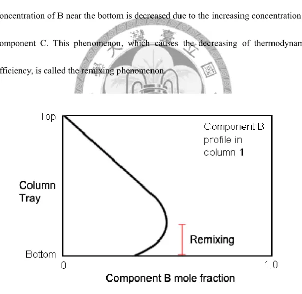
The function of first column is to separate A and B. Product A goes out from the top of the column. The liquid mixture of B and C goes into the second column from the bottom of the first column. The separation between B and C takes place in the second column. By observing the composition profile (Fig. 1.1-2), it is found that the mole fraction of B is highest at an intermediate point where no B is removed. The concentration of B near the bottom is decreased due to the increasing concentration of component C. This phenomenon, which causes the decreasing of thermodynamic efficiency, is called the remixing phenomenon.
Fig. 1.1-2 B composition profile in the first column and remixing phenomenon.
In 1949, Wright and Elizabeth [1] proposed the divided wall column (DWC). It is a kind of heat integrated column. The remixing phenomenon can be reduced by using a DWC. This will also reduce energy consumption. Because the DWC is only one column, the capital cost is also usually reduced.
Compared to classic distillation design arrangements, DWC offers the following benefits :
z high purity for all three or more product streams reached in only one column z high thermodynamic efficiency due to reduced remixing effects
z lower capital investment due to the integrated design
z lower energy requirements compared to conventional separation sequences z small footprint due to the reduced number of equipment units
z reduced maintenance costs as compared to traditional distillation sequences.
Moreover, the list of advantages can be extended when DWC is further combined with reactive distillation leading to the more integrated concept of reactive DWC. Note however that the integration of two columns into one shell leads also to changes in the operating mode and the controllability of such an integrated system.
1.2 Introduction for DWCs
All DWC columns have a wall in the column. According to the position of wall, DWCs can be classified into three types as discussed below.
1.2.1 DWCL
The first type of DWC is DWCL. The subscript means the wall is in the lower section of column. The DWCL requires two reboilers and one condenser. This construction is evolved from the indirect sequence (IS) (see Fig. 1.2-1).
Fig. 1.2-1 The evolution of DWCL
The function of the first column is to separate B and C. Product C goes out from the bottom of the column. The liquid mixture of A and B goes into the second column from the top of the first column. The separation between A and B takes place in the
second column.
If thermal coupling is used the condenser in the first column is removed. The reflux is split between the two columns at a certain tray, and the vapor is send to a certain tray in the second column. This structure is called the side striper sequence.
The side striper sequence can be divided into three parts. The reflux from the upper section flows into the left section and right section. There is a reboiler in each left and right section. Vapor from left and right section meet at the upper section. A column with a wall in the lower section has the same effect as the side striper sequence, and DWCL is thermally equivalent to the side striper sequence.
1.2.2 DWCU
The second type of DWC is DWCU. The subscript means the wall is in the upper section of column. The DWCU has one reboiler and two condensers. This construction is evolved from direct sequence (DS) (see Fig. 1.2-2)
The function of first column is the separation between A and B. Product A goes
Fig. 1.2-2 The evolution of DWCU.
If we do the thermal coupling the reboiler in the first column is removed. The vapor is from a certain tray in the second column, and the reflux is sent to a certain tray in the second column. This structure is called the side rectifier sequence. The Side Rectifier sequence can be divided into three parts. The vapor from the lower section flows into the left section and right section. There is a condenser in each left and right section. Liquid reflux from the left and right section meet at the lower section. The column with wall in the upper section has the same effect with the side rectifier sequence. And DWCU is thermally equivalent to the side rectifier sequence.
1.2.3 DWCM
The third type of DWC is DWCM. The subscript means the wall is in the middle section of column. The DWCM needs only one reboiler and one condenser. This construction is evolved from prefractionator sequence (PF) (see Fig. 1.2-3).
Fig. 1.2-3 The evolution of DWCM.
Compared with IS and DS, the difference for PF is the function of first column.
The first column separates A and C. Most of species A goes into the second column near the top of the first column. Most of species C goes into the second column near the bottom of the second column. Part of the B goes into the second column near the
in the lower section of second column. Finally, A goes out from the top of second column, B goes out from the sidedraw and C goes out from the bottom of second column.
If we do the thermal coupling, the reboiler and condenser in the first column are removed. The vapor is from a certain tray in the second column. And the reflux is sent to a certain tray in the second column. The reflux is from a certain tray in the second column. And the vapor is sent to a certain tray in the second column. This structure is called Petlyuk Column. It is also called fully thermally coupled column.
A Petlyuk column can be divided into four parts. The vapor from the lower section flows into the left section and right section and meets at the upper section.
Liquid reflux from the upper section flows into the left section and right section and meets at the lower section. The column with wall in the middle section has the same effect with Petlyuk column. And DWCM is thermally equivalent to Petlyuk column.
1.3 Literature survey
A literature study reveals that a variety of controllers are used for distillation columns. For the study of control of DWC systems, Wolff and Skogestad [2] proposed a control strategy for the ethanol/propanol/butanol system. They demonstrated that at some operating conditions the ‘holes’ phenomenon in the steady state feasibility space made the energy control structure infeasible. They used the M type of DWC systems.
Abdul Mutalib et al. [3] proposed a control strategy for methanol/2-propanol/butanol system. Their performance is just for feed flow rate disturbance and they didn’t use the other manipulated variables to minimize energy consumption. In the same year they proposed a temperature control strategy for the same system [4]. Their simulation results showed that the control structure which controls two temperatures and fixes the side stream flow does not provide effective control. They used the M type of DWC systems.
Several authors studied the design phase of the dividing-wall column in order to improve the energy efficiency [5] [6]. The design stage of a DWC is very important as
going out the top of the prefractionator. The second one is keeping the lightest component from going out the bottom of the prefractionator. The optimal solution surface of the minimal boilup is given as a function of the control variable liquid split and the design variable vapor split. They used response surfaces to describe the relationship between liquid split and energy consumption. They suggested that the control of temperature differentials is a good policy to infer composition. The system of DWC that they used was M type.
A more practical approach is suggested by Serra et al. [8]. A linearized model is used to design PI feedback controller. They proposed both PID control and DMC control strategies for three different systems. The authors used several linear analysis tools – Morari resiliency index (MRI), condition number (CN), relative gain array (RGA) to select variable pairings for three compositions control. They demonstrated that PID control gave better load disturbance than DMC control. In 2003 they concluded their previous work and gave two observations [9]. The first one is that DWC has better controllability for mixtures with ESI close to 1. The second one is that the DWC controllability at the optimal operating point is worse than the non-optimal one. The system of DWC that they used was M type.
A more advanced approach for DWC control is model predictive control (MPC) as discussed by Adrian et al. [10]. They proposed PID and MPC control strategies for butanol/petanol/hexanol system. In the PID control, the reboiler heat input was not used to control compositions, but it was in MPC control. The MPC controller outperforms a single PI loop. Three temperatures are controlled by the reflux ratios, the liquid split, and the sidedraw flow rate, respectively. The disturbance variable in this case was the feed flow rate. They used the M type of DWC systems.
Wang and Wong [11] proposed a control policy for the ethanol/1-propanol/
1-butanol system. There were large product purity deviations for feed composition disturbances. The authors suggested using a temperature-composition cascade control structure to solve the problem. The performances in dynamic simulation were good.
The system of DWC that they used was M type. Cho et al. [12] proposed a control strategy for the benzene/toluene/ p-xylene system. They proposed a profile position control scheme for the control of a DWC with vapor side draw. Relative gain array (RGA) and singular value decomposition (SVD) analysis were used to determine the optimal control configuration. Dynamic simulation showed that the profile
manipulated variables to minimize energy consumption. The system of DWC that they used was M type. Ling and Luyben [13] proposed a control strategy for the benzene/toluene/o-xylene system. They concluded that the composition of the heavy component at the top of the prefractionator is an implicit and practical way to minimize energy consumption in the presence of feed disturbances. This specific composition was controlled by the liquid split variable. They also used the M type of DWC systems. Nowadays more and more research groups focus on the controllability of divided-wall column [14] [15].
Huang et al. [16] published a report on the development of DWC systems in industry. There are also many applications of DWC in industry that have been reported. In 1980 BASF built the first commercial DWC. Presently they have twenty-eight DWC columns in operation. BASF is in the minority of chemical companies which that have used DWC systems for over ten years. They focus on the application of DWC in petrochemical field.
1.4 Motivation
Although much of the literature focuses on the control of binary distillation columns, there are only a limited number of studies on the control of DWC. And from the literature survey we notice that most research focuses on DWCM. We don’t know that whether DWCL or DWCU is more controllable than DWCM or not.
In this work, we discuss the controllability for different type of divided-wall column and different ease separation index (ESI) and different feed composition.
Finally the choice among the three configuration based on control aspect can be made.
1.5 Thesis organization
The thesis includes four chapters.
The first chapter is the introduction. Three types of DWCs and their evolutions are introduced. And we also introduce some benefits of DWCs. Then we survey the literature and expound the motivation for this work.
In the second chapter we discuss the steady-state analysis. We use shortcut method to get tray numbers of DWCs. And some linear tools – relative gain array and condition number are used for the steady-state analysis. Finally we show the results of RGA and CN.
In the third chapter we discuss the dynamic analysis. We use Aspen Plus simulator. Then we use IAE and ITAE to determine the better control structure.
Finally we show the results of different cases.
The final chapter is the conclusion. The results and discussion of previous chapters are combined. Finally we make a conclusion for the thesis.
2 Steady-State Analysis
2.1 Thermodynamic properties
In this work, we consider an ideal system where the relative volatility is constant.
We also assume constant molar flow. This means that Bvp in the Antoine equation Eq.
( 2-1) is the same for all species. Finally we can get the ideal vapor-liquid equilibrium by combing Eq. ( 2-2) to Eq. ( 2-3). P is total pressure. Ps means saturated vapor pressure. Table 2.1-1 shows the thermodynamic properties for system ESI>1. Table 2.1-2 shows the thermodynamic properties for system ESI=1. Table 2.1-3 shows the thermodynamic properties for system ESI<1. The definition of ESI is ESI= (αA/αB) / (αB/αC).
S VP, VP,
i
i i
j
lnP A B
= − T ( 2-1)
,A A ( j) ,B B( j) ,C C( j)
S S S
j T j T j T
P= X P +X P +X P ( 2-2)
S ,
, ,
j i
j i j i
y P X
= P ( 2-3)
Table 2.1-1 Thermodynamic parameters for ideal system ( ESI>1 ) ESI > 1 αA / αB / αC : 7.1 / 2.2 / 1
Avp1 (mm-Hg) 15.200702 Avp2 (mm-Hg) 14.028939 Avp3 (mm-Hg) 13.240360 Bvp (K) -2768.55 Tb(A) (K) 323.15 Tb(B) (K) 374.35 Tb(C) (K) 419.03
Table 2.1-2 Thermodynamic parameters for ideal system ( ESI=1 ) ESI = 1 αA / αB / αC : 4 / 2 / 1
Avp1 (mm-Hg) 15.200702 Avp2 (mm-Hg) 14.151030 Avp3 (mm-Hg) 13.814470 Bvp (K) -2768.55 Tb(A) (K) 323.15 Tb(B) (K) 368.27 Tb(C) (K) 385.53
Table 2.1-3 Thermodynamic parameters for ideal system ( ESI<1 ) ESI < 1 αA / αB / αC : 4 / 2.4 / 1
Avp1 (mm-Hg) 15.200702 Avp2 (mm-Hg) 14.689870 Avp3 (mm-Hg) 13.814408 Bvp (K) -2768.55 Tb(A) (K) 323.15 Tb(B) (K) 343.63 Tb(C) (K) 385.53
2.2 Shortcut method
In this work, we made the following assumptions
1. Constant relative volatility 2. Constant molar flow rate 3. Symmetric column
We consider that the relative volatility is independent of temperature and pressure. A symmetric column is a column with the same number of trays on both the left and right sides of the dividing wall. If the number of trays is different, the pressure drop may be different. This assumption is made for maintaining the same pressure on both sides of the wall.
There are a large number of degrees of freedom in DWC systems, so some simplifications are necessary. An ideal system will be used here for the whole work.
We can get the tray number for each section by shortcut design.
Chu [17] built rational models for the three configurations, the net flow compositions can be obtained in an easy way. Underwood’s method [18] will be applied to calculate minimum vapor flow for all three configurations.
Fig. 2.2-1 Shortcut design procedure for DWCL
The ways to calculate minimum vapor flow for three DWCs are proposed by Halvorsen and Skogestad [19]. The minimum vapor flow is also used to calculate the minimum reflux ratio. After that, the development of the method is based on dividing the DWC into several parts and applying the methods of Fenske-Underwood-Gilliland [20] and the Kirkbride [21] equation. The detail for the shortcut design you can refer to Chu’s thesis.
Fig. 2.2-1, Fig. 2.2-2 and Fig. 2.2-3 show the procedure of shortcut design for DWCs. The detail for the shortcut design you can refer to Chu’s thesis.
Fig. 2.2-3 Shortcut design procedure for DWCM.
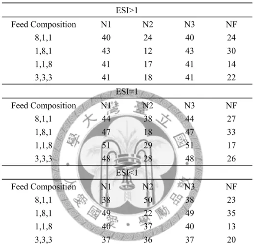
The number of trays for DWCL are given in Table 2.2-1.
Table 2.2-1 Tray number of DWCL ESI>1
Feed Composition N1 N2 N3 NF
8,1,1 40 24 40 24
1,8,1 43 12 43 30
1,1,8 41 17 41 14
3,3,3 41 18 41 22
ESI=1
Feed Composition N1 N2 N3 NF
8,1,1 44 38 44 27
1,8,1 47 18 47 33
1,1,8 51 29 51 17
3,3,3 48 28 48 26
ESI<1
Feed Composition N1 N2 N3 NF
8,1,1 38 50 38 23
1,8,1 49 22 49 35
1,1,8 40 37 40 13
3,3,3 37 36 37 20
For example, the number of feed composition 8,1,1 in the table means the mole fraction of A component is 0.8 and the mole fraction of B and C component is 0.1.
N1 is the number of tray for column 1. N2 is the number of tray for column 2.
Fig. 2.2-4 The configuration of DWCL
Fig. 2.2-5 The configuration of DWCU
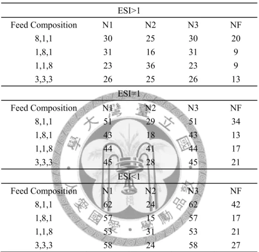
The detailed tray number for DWCU are given in Table 2.2-2.
Table 2.2-2 Tray number of DWCU ESI>1
Feed Composition N1 N2 N3 NF
8,1,1 30 25 30 20
1,8,1 31 16 31 9
1,1,8 23 36 23 9
3,3,3 26 25 26 13
ESI=1
Feed Composition N1 N2 N3 NF
8,1,1 51 29 51 34
1,8,1 43 18 43 13
1,1,8 44 41 44 17
3,3,3 45 28 45 21
ESI<1
Feed Composition N1 N2 N3 NF
8,1,1 62 24 62 42
1,8,1 57 15 57 17
1,1,8 53 31 53 21
3,3,3 58 24 58 27
N1 is the number of tray for column 1. N2 is the number of tray for column 2.
N3 is the number of tray for column 3. NF is the feed location tray number. Fig. 2.2-5
The detailed tray number for DWCM are given in Table 2.2-3.
Table 2.2-3 Tray number of DWCM ESI>1
Feed Composition N1 N2 N3 N4 NF NS
811 28 25 28 22 19 8
181 37 11 37 17 21 19
118 35 16 35 42 12 26
333 27 16 27 25 14 14
ESI=1
Feed Composition N1 N2 N3 N4 NF NS
811 43 44 43 35 29 14
181 56 14 56 20 29 33
118 37 27 37 47 12 28
333 35 25 35 30 18 20
ESI<1
Feed Composition N1 N2 N3 N4 NF NS
811 55 52 55 29 37 28
181 61 19 61 17 30 42
118 33 30 33 35 11 27
333 40 33 40 24 20 26
N1 is the number of tray for column 1. N2 is the number of tray for column 2.
N3 is the number of tray for column 3. N4 is the number of tray for column 4. NF is the feed location tray number. NS is the sidedraw stream tray number. Fig. 2.2-6 is the configuration of DWCM.
Fig. 2.2-6 The configuration of DWCM
2.3 Analysis method
2.3.1 Relative Gain Array
Bristol [22] developed a systematic approach for the analysis of multivariable process control problems. His approach requires only steady-state information (the process gain matrix K) and provides two important items of information :
1. A measure of process interactions.
2. A recommendation concerning the most effective pairing of controlled and manipulated variables.
Bristol’s approach is based on the concept of a relative gain. Consider a process with n controlled variables and n manipulated variables. The relative gain λij between a controlled variable yi and a manipulated variable uj is defined to be the dimensionless ratio of two steady-state gain :
gain loop closed
gain loop open )
/ (
) / (
−
= −
∂
∂
∂
=Δ ∂
y j i
u j i
ij y u
u
λ y ( 2-4)
for i = 1,2,…,n and j = 1,2,…,n.
In the symbol (∂yi/∂uj)u denotes a partial derivative that is evaluated with all of the manipulated variables except uj held constant. Thus, this term is the open-loop gain (or steady-state gain) between yi and uj, which corresponds to the gain matrix element Kij. Similarly, (∂yi/∂uj)y is evaluated with all of the controlled variables
except yi held constant. This situation could be achieved in practice by adjusting the other manipulated variables using controllers with integral action. Thus, (∂yi/∂uj)y can be interpreted as a closed-loop gain that indicates the effect of uj on yi when all of the other controlled variables (yi≠yj) are held constant [23].
The RGA has several important properties for steady-state process models [24]:
1. It is normalized because the sum of the elements in each row of column is equal to one.
2. The relative gain are dimensionless and thus not affected by choice of units or scaling of variables.
3. The RGA is a measure of sensitivity to element uncertainty in the gain matrix K.
The gain matrix can become singular if a single element Kij is changed to Kij = Kij(1-1/λij). Thus a large RGA element indicates that small changes in Kij can markedly change the process control characteristics.
The RGA can be calculated from the expression
H K⊗
=
Λ ( 2-5)
Where ⊗ denotes the Schur product (element by element multiplication) :
ij ij
ij =K H
λ ( 2-6)
j i
ij u
K y Δ
= Δ ( 2-7)
K T
H =( −1) ( 2-8)
Hij is an element of the transpose of the matrix inverse of K.
The RGA may be generalized to a non-square l × m matrix A by use of the pseudo inverse A+. We have [25]
)T
( )
( = ⊗ +
Λ A A A ( 2-9)
2.3.2 Condition Number
A measure of controllability is the condition number (CN). Assume that K is nonsingular. Then the condition number of K is a positive number defined as the ratio of the largest and smallest nonzero singular values :
min max
σ
=σ
CN ( 2-9)
A small value of the condition number means that the system is well conditioned.
The condition number also provides useful information about the sensitivity of the matrix properties to variations in the elements of the matrices. It is a typical index for the selection of the best set of manipulated variables [23].
2.4 Results
In section 2.4, we will show the results of relative gain array (RGA) and condition number (CN). These measures can indicate which control structure pairings are likely to work well.
These metrics are determined for three different type of divided-wall columns the L, U and M types. They are also calculated for different ease of separation index. First, the relative volatility for each component is αA / αB / αC = 7.1 / 2.2 / 1. The separation of component A from component B is easier than the separation of component B from component C. The ease separation index is bigger than one. Second, the relative volatility for each component is αA / αB / αC = 4 / 2 / 1. The difficulty of the separation of component A from component B is same as that of component B from component C. The ease separation index is equal to one. Third, the relative volatility for each component is αA / αB / αC = 4 / 2.4 / 1. The separation of component B from component C is easier than the separation of component A from component B. The ease of separation index is smaller than one.
We can make step change (+/- 1%) by using Aspen Plus and we can get the open-loop gain. Then we substitute the open-loop gain into Eq. (2-4) and get matrix K.
We can determine relative gain array by Eq. (2-5) and condition number.
2.4.1 DWCL
In this subsection we will discuss the L type of divided-wall column.
For the L type of divided-wall column, we have four manipulated variables, the reflux ratio (RR), two boilup ratios (BR1 and BR2) and split liquid (SL). So we will have four kind of control structures, RR-BR1-BR2, SL-BR1-BR2, RR-SL-BR2, RR-BR1-SL. The control structure RR-BR1-BR2 means that we control top A component by manipulating reflux ration, we control middle B component by manipulating boilup ratio one and we control bottom C component by manipulating boilup ratio two.
The following tables are the results of relative gain array and condition number for the L type:
We consider the case when ESI>1 (αA / αB / αC : 7.1 / 2.2 / 1).
If there is more lightest component in the feed: From Table 2.4-1, we can see that the RGA and CN show the control structure RR-BR1-BR2 is likely to work well.
Table 2.4-1 RGA and CN analysis for DWCL, ESI>1, F(8,1,1)
RGA CN RR BR1 BR2
1.0976 XA 1.0376 0.0053 -0.0429
XB 0.0058 0.9902 0.0040 XC -0.0434 0.0045 1.0389
SL BR1 BR2
1.5583 XA 0.8469 -0.0198 0.1729
XB -0.0212 1.0210 0.0002 XC 0.1743 -0.0012 0.8268
RR SL BR2
1.9352 XA 0.8175 0.1797 0.0029
XB 0.1915 0.6821 0.1264 XC -0.0090 0.1383 0.8707
RR BR1 SL
1.5390 XA 0.8312 0.0003 0.1684
XB -0.0004 1.0229 -0.0226 XC 0.1691 -0.0233 0.8541
NRGA
RR BR1 BR2 SL XA 0.9107 0.0023 -0.0165 0.1036 XB 0.0568 0.7180 0.0377 0.1875 XC -0.0268 0.0023 0.9577 0.0667
If there is more middle component in the feed: From Table 2.4-2, we can see that the RGA and CN show the control structure RR-BR1-BR2 and RR-SL-BR2 are both likely to work well.
Table 2.4-2 RGA and CN analysis for DWCL, ESI>1, F(1,8,1)
RGA CN RR BR1 BR2
1.1226 XA 1.0498 -0.0477 -0.0020
XB -0.0477 1.0803 -0.0326 XC -0.0021 -0.0325 1.0346
SL BR1 BR2
1.9816 XA 1.3916 -0.4177 0.0261
XB -0.4746 1.4702 0.0044 XC 0.0829 -0.0525 0.9695
RR SL BR2
1.4769 XA 1.1852 -0.1796 -0.0056
XB -0.1797 1.3147 -0.1350 XC -0.0055 -0.1352 1.1407
RR BR1 SL
1.8545 XA 0.9745 -0.0743 0.0997
XB -0.0057 1.4239 -0.4183 XC 0.0311 -0.3497 1.3185
NRGA
RR BR1 BR2 SL XA 1.1058 -0.0280 -0.0035 -0.0743
If there is more heaviest component in the feed: From Table 2.4-3, we can see that the RGA and CN show the control structure RR-BR1-BR2 and RR-SL-BR2 are both likely to work well.
Table 2.4-3 RGA and CN analysis for DWCL, ESI>1, F(1,1,8)
RGA CN
RR BR1 BR2
1.9876 XA 1.2612 0.0238 -0.2850
XB 0.1678 0.8956 -0.0635 XC -0.4291 0.0805 1.3485
SL BR1 BR2
27.8160 XA 1.4041 -2.8544 2.4502
XB 0.0322 15.5269 -14.5591 XC -0.4363 -11.6725 13.1088
RR SL BR2
1.9983 XA 1.2736 0.0280 -0.3016
XB 0.1581 0.8998 -0.0579 XC -0.4317 0.0722 1.3595
RR BR1 SL
19.2168 XA 1.0484 -0.4817 0.4333
XB 0.0565 10.3006 -9.3571 XC -0.1049 -8.8189 9.9238
NRGA
RR BR1 BR2 SL
XA 1.2734 0.0005 -0.3013 0.0275 XB 0.1581 -0.0009 -0.0579 0.9007 XC -0.4316 0.0039 1.3590 0.0687
If there is equivalent component in the feed: From Table 2.4-4 we can see that the RGA and CN show the control structure RR-BR1-BR2 and RR-SL-BR2 are both likely to work well.
Table 2.4-4 RGA and CN analysis for DWCL, ESI>1, F(3,3,3)
RGA CN RR BR1 BR2
1.1400 XA 1.0081 0.0288 -0.0369
XB 0.0383 0.9623 -0.0006 XC -0.0465 0.0089 1.0376
SL BR1 BR2
2.3810 XA 0.9890 -0.2016 0.2126
XB -0.2683 1.2683 -0.0001 XC 0.2793 -0.0667 0.7874
RR SL BR2
1.4152 XA 0.8821 0.1236 -0.0057
XB 0.1589 0.8435 -0.0024 XC -0.0410 0.0329 1.0081
RR BR1 SL
2.0382 XA 0.8589 -0.0053 0.1464
XB -0.0052 1.3101 -0.3049 XC 0.1463 -0.3048 1.1585
NRGA
Next we consider the case when ESI=1 (αA / αB / αC : 4 / 2 / 1).
If there is more lightest component in the feed: From Table 2.4-5, we can see that the RGA and CN show the control structure RR-BR1-BR2 is likely to work well.
Table 2.4-5 RGA and CN analysis for DWCL, ESI=1, F(8,1,1)
RGA CN RR BR1 BR2
1.1343 XA 1.0524 0.0047 -0.0571
XB 0.0044 0.9836 0.0121 XC -0.0568 0.0117 1.0450
SL BR1 BR2
2.8397 XA 0.7085 -0.0313 0.3228
XB -0.0313 1.0329 -0.0016 XC 0.3228 -0.0016 0.6788
RR SL BR2
2.6647 XA 0.9154 0.0923 -0.0076
XB 0.0916 0.6243 0.2841 XC -0.0069 0.2834 0.7235
RR BR1 SL
1.3044 XA 0.8942 -0.0007 0.1065
XB 0.0005 1.0271 -0.0277 XC 0.1052 -0.0264 0.9212
NRGA
RR BR1 BR2 SL XA 0.9805 0.0022 -0.0311 0.0484 XB 0.0245 0.7570 0.0747 0.1438 XC -0.0350 0.0066 0.9044 0.1239
If there is more middle component in the feed: From Table 2.4-6, we can see that the RGA and CN show the control structure RR-BR1-BR2 is likely to work well.
Table 2.4-6 RGA and CN analysis for DWCL, ESI=1, F(1,8,1)
RGA CN RR BR1 BR2
1.2223 XA 1.0869 -0.0842 -0.0027
XB -0.0820 1.1469 -0.0649 XC -0.0049 -0.0627 1.0676
SL BR1 BR2
2.2669 XA 1.4930 -0.5151 0.0221
XB -0.6238 1.6104 0.0134 XC 0.1308 -0.0952 0.9644
RR SL BR2
1.8167 XA 1.2992 -0.2916 -0.0076
XB -0.2849 1.5434 -0.2585 XC -0.0143 -0.2518 1.2661
RR BR1 SL
2.0696 XA 0.9683 -0.1312 0.1630
XB -0.0140 1.5309 -0.5169 XC 0.0458 -0.3997 1.3539
NRGA
RR BR1 BR2 SL XA 1.0858 -0.0846 -0.0027 0.0016
If there is more heaviest component in the feed: From Table 2.4-7, we can see that the RGA and CN show the control structure RR-BR1-BR2 and RR-SL-BR2 are both likely to work well.
Table 2.4-7 RGA and CN analysis for DWCL, ESI=1, F(1,1,8)
RGA CN RR BR1 BR2
1.8024 XA 1.0889 0.0286 -0.1176
XB 0.2432 0.8625 -0.1057 XC -0.3321 0.1089 1.2233
SL BR1 BR2
3.0412 XA -0.1503 0.2431 0.9072
XB 1.8594 -0.8641 0.0046 XC -0.7091 1.6209 0.0882
RR SL BR2
1.7773 XA 1.2343 0.0201 -0.2544
XB 0.1217 0.9289 -0.0506 XC -0.3561 0.0511 1.3050
RR BR1 SL
2.6858 XA 0.9640 0.0533 -0.0172
XB 0.0102 -0.7916 1.7814 XC 0.0258 1.7384 -0.7642
NRGA
RR BR1 BR2 SL XA 1.2133 0.0041 -0.2346 0.0172 XB 0.1196 -0.0152 -0.0496 0.9453 XC -0.3463 0.0443 1.2718 0.0303
If there is equivalent component in the feed: From Table 2.4-8, we can see that the RGA and CN show the control structure RR-BR1-BR2 is likely to work well.
.
Table 2.4-8 RGA and CN analysis for DWCL, ESI=1, F(3,3,3)
RGA CN RR BR1 BR2
1.1729 XA 1.0210 0.0292 -0.0503
XB 0.0407 0.9581 0.0012 XC -0.0617 0.0127 1.0491
SL BR1 BR2
5.9532 XA 0.7827 -0.1829 0.4002
XB -0.2542 1.2546 -0.0004 XC 0.4715 -0.0717 0.6002
RR SL BR2
1.4225 XA 0.8803 0.1079 0.0118
XB 0.1722 0.8213 0.0065 XC -0.0525 0.0708 0.9817
RR BR1 SL
1.5703 XA 0.9071 0.0056 0.0873
XB 0.0104 1.1790 -0.1893 XC 0.0825 -0.1845 1.1020
NRGA
RR BR1 BR2 SL XA 0.8728 -0.0016 0.0151 0.1136
Next we consider the case when ESI<1 (αA / αB / αC : 4 / 2.4 / 1).
If there is more lightest component in the feed: From Table 2.4-9, we can see that the RGA and CN show the control structure RR-BR1-BR2 is likely to work well.
Table 2.4-9 RGA and CN analysis for DWCL, ESI<1, F(8,1,1)
RGA CN RR BR1 BR2
1.6706 XA 0.8384 0.2247 -0.0631
XB 0.1515 0.7572 0.0913 XC 0.0101 0.0181 0.9718
SL BR1 BR2
1.8784 XA -0.1152 1.3612 -0.2460
XB 1.0746 -0.3765 0.3019 XC 0.0407 0.0153 0.9441
RR SL BR2
2.0227 XA 1.0042 0.0228 -0.0270
XB 0.0503 0.7177 0.2320 XC -0.0545 0.2595 0.7950
RR BR1 SL
1.7007 XA 1.1278 -0.1675 0.0398
XB 0.2172 1.2489 -0.4661 XC -0.3449 -0.0814 1.4263
NRGA
RR BR1 BR2 SL XA 0.8465 0.2138 -0.0614 0.0011 XB 0.1159 0.4913 0.1407 0.2520 XC -0.0133 0.0115 0.9077 0.0940
If there is more middle component in the feed: From Table 2.4-10, we can see that the RGA and CN show the control structure RR-BR1-BR2 is likely to work well.
Table 2.4-10 RGA and CN analysis for DWCL, ESI<1, F(1,8,1)
RGA CN RR BR1 BR2
1.0634 XA 1.0333 -0.0269 -0.0065
XB -0.0317 1.0231 0.0085 XC -0.0017 0.0037 0.9979
SL BR1 BR2
1.5748 XA 1.0420 -0.1467 0.1047
XB -0.1652 1.1628 0.0024 XC 0.1233 -0.0161 0.8929
RR SL BR2
1.5476 XA 1.2649 -0.2335 -0.0314
XB -0.2636 1.2103 0.0532 XC -0.0014 0.0232 0.9782
RR BR1 SL
1.4718 XA 0.9731 -0.0338 0.0608
XB 0.0127 1.2188 -0.2316 XC 0.0142 -0.1850 1.1708
NRGA
RR BR1 BR2 SL XA 1.0330 -0.0269 -0.0064 0.0004
If there is more heaviest component in the feed: From Table 2.4-11, we can see that the RGA and CN show the control structure RR-SL-BR2 is likely to work well.
Table 2.4-11 RGA and CN analysis for DWCL, ESI<1, F(1,1,8)
RGA CN RR BR1 BR2
2.3833 XA 1.0429 0.1122 -0.1551
XB 0.3878 0.8471 -0.2349 XC -0.4307 0.0407 1.3900
SL BR1 BR2
4.8683 XA -0.3205 -0.4930 1.8136
XB -2.0526 2.6818 0.3708 XC 3.3731 -1.1888 -1.1844
RR SL BR2
2.0806 XA 0.8495 -0.0594 0.2099
XB 0.5669 0.9477 -0.5145 XC -0.4164 0.1117 1.3047
RR BR1 SL
2.6730 XA 0.9607 0.0645 -0.0252
XB 0.2374 1.5586 -0.7960 XC -0.1981 -0.6231 1.8212
NRGA
RR BR1 BR2 SL XA 0.8580 0.0049 0.1939 -0.0568 XB 0.4831 0.3963 -0.3837 0.5044 XC -0.3756 -0.1165 1.0607 0.4315
If there is equivalent component in the feed: From Table 2.4-12, we can see that the RGA and CN show the control structure RR-SL-BR2 is likely to work well.
Table 2.4-12 RGA and CN analysis for DWCL, ESI<1, F(3,3,3)
RGA CN RR BR1 BR2
7.5223 XA 0.5804 0.4177 0.0019
XB 0.4570 0.5680 -0.0250 XC -0.0374 0.0143 1.0231
SL BR1 BR2
1.1856 XA -0.0169 1.0056 0.0113
XB 1.0975 -0.0763 -0.0212 XC -0.0806 0.0707 1.0099
RR SL BR2
1.1086 XA 0.9928 0.0120 -0.0048
XB 0.0541 0.9676 -0.0217 XC -0.0469 0.0204 1.0265
RR BR1 SL
29.5565 XA 0.6967 0.2999 0.0034
XB -2.5511 -3.6726 7.2237 XC 2.8543 4.3728 -6.2271
NRGA
RR BR1 BR2 SL XA 0.7576 0.2382 -0.0010 0.0052
2.4.2 DWCU
In this subsection we will discuss the U type of divided-wall column.
For the U type of divided-wall column, we have four manipulated variables, two reflux ratios (RR1 and RR2), one boilup ratio (BR) and split vapor (SV). But in practical industrial, the split vapor is hard to control. So we get rid of the manipulated variable split vapor. We have only left one control structure RR1-RR2-BR to control the A component in top stream, the B component in middle stream and the C component in bottom stream, respectively. So it is unnecessary to compare the relative gain array and condition number here.
2.4.3 DWCM
In this subsection we will discuss the M type of divided-wall column.
For the M type of divided-wall column, we have five manipulated variables, the reflux ratios (RR), the sidedraw stream flowrate (S), the boilup ratio (BR), split liquid (SL) and split vapor (SV). But in practical industrial, the split vapor is hard to control.
So we do not consider split vapor as a manipulated variable.
The following tables are the results of relative gain array and condition number for the M type:
We consider the case when ESI>1 (αA / αB / αC : 7.1 / 2.2 / 1).
If there is more lightest component in the feed: From Table 2.4-13, we can see that the RGA and CN show the control structure S-SL-BR is likely to work well.
Table 2.4-13 RGA and CN analysis for DWCM, ESI>1, F(8,1,1)
RGA CN RR S BR
4.9421 XA 0.4911 0.6123 -0.1034
XB 0.5918 0.3233 0.0848 XC -0.0829 0.0644 1.0186
SL S BR
2.6343 XA 0.3236 0.6599 0.0165
XB 0.6975 0.2736 0.0289 XC -0.0211 0.0665 0.9546
RR SL BR
10.0622 XA 6.8101 -4.1641 -1.6460
XB -3.2551 4.5338 -0.2787 XC -2.5550 0.6303 2.9248
RR S SL
3.2731 XA 0.0676 0.6533 0.2791
XB -0.3056 0.2479 1.0577 XC 1.2380 0.0988 -0.3368
NRGA
RR S BR SL XA 0.0952 0.6263 -0.0681 0.3467 XB 0.2233 0.3074 0.0669 0.4024 XC -0.0079 0.0652 0.9948 -0.0521
If there is more middle component in the feed: From Table 2.4-14 , we can see that the RGA and CN show the control structure RR-S-BR is likely to work well.
Table 2.4-14 RGA and CN analysis for DWCM, ESI>1, F(1,8,1)
RGA CN RR S BR
1.6110 XA 0.8505 0.1360 0.0135
XB 0.1492 0.7496 0.1012 XC 0.0003 0.1144 0.8853
SL S BR
5.3665 XA -0.7346 0.6952 1.0394
XB 1.8749 0.1997 -1.0745 XC -0.1403 0.1051 1.0352
RR SL BR
4.2795 XA 1.0574 0.1786 -0.2360
XB -0.0542 2.5555 -1.5013 XC -0.0032 -1.7341 2.7373
RR S SL
1.8158 XA 0.8617 0.1286 0.0097
XB 0.1364 0.7023 0.1613 XC 0.0019 0.1691 0.8290
NRGA
RR S BR SL XA 0.8499 0.1364 0.0142 -0.0005
If there is more heaviest component in the feed: From Table 2.4-15, we can see that the RGA and CN show the control structure BR-SL-S and RR-SL-S are both likely to work well.
Table 2.4-15 RGA and CN analysis for DWCM, ESI>1, F(1,1,8)
RGA CN RR S BR
3.1518 XA 0.8748 0.1299 -0.0047
XB 0.4198 0.0949 0.4853 XC -0.2946 0.7751 0.5194
SL S BR
1.5879 XA 0.0366 0.1213 0.8421
XB 0.8777 0.1230 -0.0007 XC 0.0857 0.7557 0.1586
RR SL BR
25.3078 XA -12.2905 0.5510 12.7395
XB 1.8395 -2.9683 2.1288 XC 11.4509 3.4173 -13.8683
RR S SL
1.6114 XA 0.8699 0.1299 0.0002
XB 0.0006 0.1230 0.8764 XC 0.1295 0.7471 0.1234
NRGA
RR S BR SL XA 0.5120 0.1247 0.3411 0.0223 XB 0.0258 0.1215 0.0229 0.8299 XC 0.0904 0.7520 0.0557 0.1019
If there is equivalent component in the feed: From Table 2.4-16, we can see that the RGA and CN show the control structure S-RR-BR is likely to work well.
Table 2.4-16 RGA and CN analysis for DWCM, ESI>1, F(3,3,3)
RGA CN RR S BR
3.9201 XA 0.3710 0.4851 0.1438
XB 0.7004 0.1784 0.1211 XC -0.0715 0.3364 0.7350
SL S BR
5.7614 XA 0.0204 0.5405 0.4391
XB 0.9255 0.1071 -0.0326 XC 0.0541 0.3524 0.5935
RR SL BR
5.7433 XA 3.6243 -0.1789 -2.4454
XB -1.0512 2.3146 -0.2634 XC -1.5731 -1.1357 3.7088
RR S SL
9.3364 XA 0.5517 0.4582 -0.0099
XB 0.1486 0.1222 0.7292 XC 0.2997 0.4196 0.2807
NRGA
RR S BR SL XA 0.3217 0.4925 0.1831 0.0027
Next we consider the case when ESI=1 (αA / αB / αC : 4 / 2 / 1).
If there is more lightest component in the feed: From Table 2.4-17, we can see that the RGA and CN show the control structure S-SL-BR and S-SL-RR are both likely to work well.
Table 2.4-17 RGA and CN analysis for DWCM, ESI=1, F(8,1,1)
RGA CN RR S BR
8.6930 XA 0.5098 0.6770 -0.1869
XB 0.3979 0.2631 0.3391 XC 0.0923 0.0599 0.8478
SL S BR
2.1816 XA 0.2714 0.7031 0.0255
XB 0.7227 0.2376 0.0396 XC 0.0059 0.0593 0.9348
RR SL BR
20.6965 XA 13.7625 -7.0546 -5.7079
XB -3.7160 7.4732 -2.7571 XC -9.0464 0.5814 9.4650
RR S SL
2.0134 XA 0.0613 0.7000 0.2388
XB -0.0527 0.2342 0.8184 XC 0.9914 0.0658 -0.0572
NRGA
RR S BR SL XA 0.0363 0.7012 0.0104 0.2520 XB -0.0044 0.2373 0.0364 0.7307 XC 0.1216 0.0601 0.8201 -0.0019
If there is more middle component in the feed: From Table 2.4-18, we can see that the RGA and CN show the control structure RR-S-BR is likely to work well.
Table 2.4-18 RGA and CN analysis for DWCM, ESI=1, F(1,8,1)
RGA CN RR S BR
1.3627 XA 0.9777 0.0983 -0.0760
XB 0.0948 0.8893 0.0160 XC -0.0725 0.0125 1.0600
SL S BR
3.4628 XA 0.9520 0.3243 -0.2763
XB 0.3097 0.6507 0.0396 XC -0.2617 0.0251 1.2366
RR SL BR
2.1509 XA 1.4028 -0.4139 0.0111
XB -0.2584 1.1543 0.1041 XC -0.1444 0.2595 0.8848
RR S SL
1.9422 XA 1.3487 0.0125 -0.3612
XB 0.1588 1.0506 -0.2094 XC -0.5075 -0.0631 1.5706
NRGA
RR S BR SL XA 0.9637 0.1015 -0.0788 0.0136
If there is more heaviest component in the feed: From Table 2.4-19, we can see that the RGA and CN show the control structure RR-SL-S is likely to work well.
Table 2.4-19 RGA and CN analysis for DWCM, ESI=1, F(1,1,8)
RGA CN RR S BR
10.6847 XA -2.8271 0.5055 3.3216
XB 3.8484 -0.2547 -2.5937 XC -0.0213 0.7491 0.2721
SL S BR
1.4269 XA -0.0020 0.1495 0.8526
XB 1.0019 -0.0006 -0.0012 XC 0.0002 0.8511 0.1487
RR SL BR
1.3637 XA 1.1868 -0.0029 -0.1839
XB -0.0093 1.0043 0.0050 XC -0.1775 -0.0014 1.1789
RR S SL
1.0576 XA 0.9762 0.0265 -0.0028
XB -0.0019 -0.0005 1.0023 XC 0.0256 0.9740 0.0004
NRGA
RR S BR SL XA 0.6467 0.0680 0.2878 -0.0025 XB -0.0033 -0.0004 0.0010 1.0027 XC -0.0434 0.6430 0.4006 -0.0002
If there is equivalent component in the feed: From Table 2.4-20, we can see that the RGA and CN show the control structure RR-SL-BR and S-SL-BR are both likely to work well.
Table 2.4-20 RGA and CN analysis for DWCM, ESI=1, F(3,3,3)
RGA CN RR S BR
59.1920 XA 2.1061 -0.1341 -0.9719
XB -1.1054 0.6854 1.4201 XC -0.0006 0.4487 0.5519
SL S BR
7.8357 XA -0.0126 0.5864 0.4262
XB 1.0126 -0.0356 0.0230 XC 0.0000 0.4492 0.5509
RR SL BR
2.5086 XA 1.7140 -0.0023 -0.7117
XB -0.0545 0.9627 0.0919 XC -0.6595 0.0397 1.6198
RR S SL
3.4076 XA 0.6420 0.3668 -0.0087
XB 0.0182 -0.0474 1.0292 XC 0.3398 0.6807 -0.0205
NRGA
Next we consider the case when ESI=1 (αA / αB / αC : 4 / 2.4 / 1).
If there is more lightest component in the feed: From Table 2.4-21, we can see that the RGA and CN show the control structure S-SL-BR and S-SL-RR are both likely to work well.
Table 2.4-21 RGA and CN analysis for DWCM, ESI<1, F(8,1,1)
RGA CN RR S BR
10.2864 XA 0.7541 0.5044 -0.2585
XB 0.3618 0.4540 0.1842 XC -0.1159 0.0415 1.0744
SL S BR
2.8311 XA 0.3003 0.6396 0.0601
XB 0.6893 0.3159 -0.0053 XC 0.0104 0.0445 0.9452
RR SL BR
4.9975 XA 3.5687 -1.1208 -1.4479
XB -0.8276 2.2662 -0.4386 XC -1.7411 -0.1454 2.8865
RR S SL
2.7886 XA 0.1423 0.6141 0.2436
XB 0.0101 0.3198 0.6702 XC 0.8477 0.0661 0.0862
NRGA
RR S BR SL XA 0.1696 0.6092 -0.0116 0.2327 XB -0.0262 0.3059 -0.0190 0.7392 XC 0.1592 0.0485 0.7676 0.0246
If there is more middle component in the feed: From Table 2.4-22, we can see that the RGA and CN show the control structure RR-S-BR is likely to work well.
Table 2.4-22 RGA and CN analysis for DWCM, ESI<1, F(1,8,1)
RGA CN RR S BR
1.2232 XA 1.0099 0.0439 -0.0538
XB 0.0305 0.9059 0.0636 XC -0.0404 0.0501 0.9903
SL S BR
11.6723 XA 7.8978 -1.8711 -5.0266
XB -3.7512 3.0213 1.7299 XC -3.1466 -0.1501 4.2967
RR SL BR
2.5565 XA 0.9867 0.1812 -0.1679
XB 0.0435 1.6065 -0.6501 XC -0.0303 -0.7877 1.8180
RR S SL
1.4709 XA 1.0208 0.0647 -0.0855
XB 0.0316 0.8252 0.1431 XC -0.0525 0.1101 0.9424
NRGA
RR S BR SL XA 1.0104 0.0448 -0.0516 -0.0035
If there is more heaviest component in the feed: From Table 2.4-23, we can see that the RGA and CN show the control structure RR-SL-S is likely to work well.
Table 2.4-23 RGA and CN analysis for DWCM, ESI<1, F(1,1,8)
RGA CN RR S BR
2.8543 XA -0.6428 0.2379 1.4048
XB 1.5927 -0.0731 -0.5197 XC 0.0501 0.8351 0.1148
SL S BR
1.6217 XA -0.0017 0.1919 0.8099
XB 1.0024 -0.0021 -0.0003 XC -0.0007 0.8102 0.1905
RR SL BR
4.3132 XA 2.6763 -0.0089 -1.6674
XB -0.0468 1.0319 0.0149 XC -1.6296 -0.0229 2.6525
RR S SL
1.3461 XA 0.8749 0.1291 -0.0041
XB -0.0010 -0.0020 1.0030 XC 0.1261 0.8729 0.0010
NRGA
RR S BR SL XA 0.6467 0.1455 0.2112 -0.0035 XB -0.0054 -0.0018 0.0014 1.0058 XC -0.1267 0.7472 0.3819 -0.0024
If there is equivalent component in the feed: From Table 2.4-24, we can see that the RGA and CN show the control structure RR-SL-BR is likely to work well.
Table 2.4-24 RGA and CN analysis for DWCM, ESI<1, F(3,3,3)
RGA CN RR S BR
20.6778 XA 0.7364 0.3333 -0.0697
XB 0.2233 0.3047 0.4720 XC 0.0404 0.3619 0.5977
SL S BR
5.7013 XA 0.2874 0.4498 0.2628
XB 0.7191 0.1982 0.0828 XC -0.0064 0.3520 0.6545
RR SL BR
4.0138 XA 2.8434 -0.8223 -1.0211
XB -0.4153 2.0567 -0.6414 XC -1.4281 -0.2343 2.6624
RR S SL
9.2548 XA 0.5820 0.3577 0.0602
XB -0.0475 0.1755 0.8719 XC 0.4655 0.4667 0.0678
NRGA
RR S BR SL XA 0.5776 0.3584 0.0020 0.0620
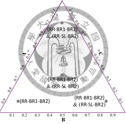
2.5 Summary
From the results of RGA and CN of DWCL we can see that in most cases the control structures RR-BR1-BR2 and RR-SL-BR2 are preferred. (see Fig. 2.5-1, Fig.
2.5-2, Fig. 2.5-3)
Fig. 2.5-1 Results of RGA and CN for DWCL of ESI>1
Fig. 2.5-2 Results of RGA and CN for DWCL of ESI=1
For DWCU, we have the only control structure RR1-RR2-BR.
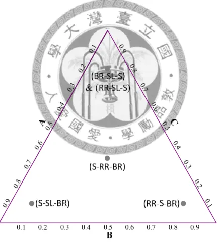
From the results of RGA and CN of DWCM we can see that if there are more A component in the feed, it prefers the control structure S-SL-BR or S-SL-RR. If there are more B component in the feed, it prefers the control structure RR-S-BR. If there are more C component in the feed, it prefers the control structure RR-SL-S. (see Fig.
2.5-4, Fig. 2.5-5, Fig. 2.5-6)
Fig. 2.5-4 Results of RGA and CN for DWCM of ESI>1
Fig. 2.5-5 Results of RGA and CN for DWCM of ESI=1