New spectroscopic data, spin-orbit functions, and global analysis of data on the A(1)Sigma(+)(u) and b(3)Pi(u) states of Na-2

New spectroscopic data, spin-orbit functions, and global analysis of data on the A

¹

⌺

_u⁺

and b

³

⌸

_u

states of Na

₂

P. Qi, J. Bai, E. Ahmed, A. M. Lyyra, and S. Kotochigova

Physics Department, Temple University, Philadelphia, Pennsylvania 19122-6082 A. J. Ross and C. Effantin

Laboratoire de Spectrométrie Ionique et Moléculaire (UMR 5579 CNRS - Université Lyon 1), 43 Boulevard du 11 novembre 1918, 69622 Villeurbanne Cedex, France

P. Zalicki

KLA-Tencor, 160 Rio Robles, San Jose, California 95134 J. Vigué

Laboratoire Collisions, Agrégats, Réactivité (UMR 5589, CNRS - Université Paul Sabatier, Toulouse 3) IRSAMC, 31062 Toulouse Cedex 9, France

G. Chawla and R. W. Field

Department of Chemistry 6-219, Massachusetts Institute of Technology, Cambridge, Massachusetts 02139 T.-J. Whang

Department of Chemistry, National Cheng Kung University, Tainan, Taiwan 70101, Republic of China W. C. Stwalley

Department of Physics, University of Connecticut, Storrs, Connecticut 06269-3046 H. Knöckel and E. Tiemann

Institut für Quantenoptik, Universität Hannover, Welfengarten 1, 30167 Hannover, Germany J. Shang and L. Li

Department of Physics, Tsinghua University, Beijing 100084, China and Key Laboratory of Atomic and Molecular Nanosciences, Tsinghua University, Beijing 100084, China

T. Bergeman

Department of Physics and Astronomy, SUNY, Stony Brook, New York 11794-3800 共Received 5 March 2007; accepted 15 May 2007; published online 23 July 2007兲

The lowest electronically excited states of Na₂are of interest as intermediaries in the excitation of higher states and in the development of methods for producing cold molecules. We have compiled previously obtained spectroscopic data on the A¹⌺u+and b³⌸ustates of Na₂from about 20 sources, both published and unpublished, together with new sub-Doppler linewidth measurements of about 15 000 A←X transitions using polarization spectroscopy. We also present new ab initio results for the diagonal and off-diagonal spin-orbit functions. The discrete variable representation is used in conjunction with Hund’s case a potentials plus spin-orbit effects to model data extending fromv

= 0 to very close to the 3²S + 3²P_1/2limit. Empirical estimates of the spin-orbit functions agree well with the ab initio functions for the accessible values of R. The potential function for the A state includes an exchange potential for S + P atoms, with a fitted coefficient somewhat larger than the predicted value. Observed and calculated term values are presented in an auxiliary共EPAPS兲 file as a database for future studies on Na₂. © 2007 American Institute of Physics.

关DOI:10.1063/1.2747595兴

I. INTRODUCTION

There are several reasons for reexamining the spectro- scopic data on the lowest excited states, A¹⌺u+and b³⌸u, of the Na₂molecule. First, there currently is widespread interest in producing ultracold ground state molecules,¹and there are advantages in starting with laser-cooled atoms. Subsequent steps of photoassociation and Raman transfer to the ground state require accurate knowledge of excited state level struc- ture. Second, these lowest excited states provide the most widely used pathways to higher states, and levels with mixed singlet-triplet character are of particular interest as “window

states.”² For any experiment using these lowest excited states, it is essential to have accurate term values and to know the composition of the eigenstates of interest. Third, the renewed interest in photoassociation and excitation of alkali molecules for diverse reasons has raised general ques- tions about how to model spin-orbit functions and Born- Oppenheimer potentials, including the exchange and disper- sion terms. For such questions, Na₂ is a valuable test case because it is relatively simple, with relatively small spin- orbit effects, and also the experimental data is most abun- dant. In view of the above, in this study we have compiled

0021-9606/2007/127共4兲/044301/17/$23.00 127, 044301-1 © 2007 American Institute of Physics

fragmentary published and unpublished information together with extensive new sub-Doppler measurements of A←X transitions to assemble a comprehensive picture of these states. New ab initio spin-orbit functions play an essential role in the analysis.

The A¹⌺u

+state of Na₂ first attracted interest because of its unexpectedly robust magnetic rotation spectrum 共MRS兲,^3,4 which contrasted with predictions for a pure ¹⌺u+

state, which would have negligible magnetic moment. With the help of Mulliken’s survey of molecular orbital structure of diatomic molecules,⁵the observed MRS was attributed to perturbations by a slightly lower-lying³⌸ustate.⁴Vibrational numbering of the A state was determined in Ref.4, and in- formation on the ³⌸u perturber was deduced by Carroll.⁶ Vibrational numbering of the b state was established much later by Li et al.⁷

More detailed study of the perturbations in the Na₂ A

←X spectrum was apparently carried out first by Kusch and Hessel⁸in 1976, based on absorption spectra obtained with a grating spectrograph. They reported detailed rotational struc- ture near perturbation crossings inv = 0 and 1 of the A state, but did not report interaction parameters.

Since the earliest days of laser spectroscopy, there have been many high quality observations of restricted sets of levels of the Na₂A and b states, depending on the resources of each laboratory. The first laser spectroscopic study of the Na₂A state by Kaminsky in Schawlow’s laboratory reported 共also in 1976兲 the observation of some 114 A←X spectral lines.^9,10It was noted in Ref.10that one level was perturbed.

Slightly later Engelke et al.,¹¹ Atkinson et al.,^12,13 and Shimizu and Shimizu¹⁴observed transitions to various levels of the b state, using lasers and molecular beams. A⬃b cou- pling parameters were extracted, and the b state spin-orbit splitting was observed.

A systematic study of A⬃b perturbations in low vibra- tional levels of the A state was presented by Effantin et al.¹⁵ and Babaky.¹⁶They used Fourier transform spectroscopy to resolve emission from the 共2兲 ¹⌺g+ state. All-optical triple resonance¹⁷ and perturbation-facilitated optical-optical double resonance methods allowed Whang et al.^18,19 to ob- tain information on lower and higher vibrational levels of the b state. More recently, Zalicki et al.²⁰obtained precision la- ser molecular beam data on levels of the b³⌸u state that perturb the lower vibrational levels of the A state. Notable among other studies cited in Sec. II are those by Chawla and co-workers,^21,22 who measured two rotational levels in each of the A state vibrational levels v = 62– 105 by modulated gain spectroscopy, and by Tiemann et al.,²³who excited step- wise via X共v=31兲 up to the dissociation limit.

There is some urgency in making the present compila- tion because some of the raw spectroscopic data predate the era of electronic information storage and are available only as hard copy output, or as handwritten lists, which are in danger of being lost forever 共as appears to be the case for some of the raw spectroscopic data associated with several of the sources listed below兲. A comprehensive survey is also useful in exposing gaps in the spectroscopic information. In fact, gaps in the original data for this survey inspired a suc- cession of efforts to supplement the available data, as dis-

cussed below. These efforts culminated in a comprehensive study of the Na₂ A←X absorption spectrum using polariza- tion spectroscopy to provide sub-Doppler linewidths for mol- ecules in a heat pipe oven.²⁴The assignment of some 15 000 transitions 共for 13 500 lines兲 obtained by this means was facilitated first by retrieving handwritten tables of line posi- tions used for Ref.15, and second by an extensive absorption spectrum of the A←X bands, in addition to the other data available at the time.

Recent developments make a global analysis possible.

共1兲 A direct fit to analytic potential functions in place of a fit to Dunham parameters using Rydberg-Klein-Rees 共RKR兲 procedures eliminates the semiclassical approximation and is less subject to divergence and instability at large R values.

Similar approaches have been used recently by many authors including those of Refs.25–29. For the models used here, it is thereby easier for the “short-range” potential to extend into the region in which there is only a small overlap of the atomic wave functions. 共2兲 In place of Numerov or other methods for obtaining individual eigenfunctions for a band- by-band analysis, it is now possible to obtain eigenvalues by matrix diagonalization of a Hamiltonian for coupled poten- tials. The discrete variable representation 共DVR兲 关also known as the Fourier Grid Hamiltonian 共FGH兲 method兴^30–32 is used here as in Refs. 27 and29. This numerical method can be used to take into account coupling effects between entire manifolds of discrete and continuum states. In heavier alkali dimers, for which spin-orbit coupling functions in- crease in magnitude, this method or the equivalent becomes essential. A two-channel version of the DVR/FGH approach was, in fact, applied to the A and b states of Na₂ in 1995,³² with fewer experimental data available than in the present work. To reduce the required number of mesh points, the mapped FGH method^33,34has been used, as well as analytic scaling,³⁵which we adopt here. In a sense, FGH/DVR meth- ods present a new paradigm for modeling diatomic spectra, and this study represents another test case.

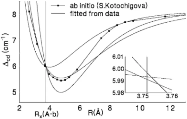
The spin-orbit functions, diagonal and off-diagonal, are clearly essential in this analysis. In the earlier stages of this work, we were able to extract empirical information on spin- orbit functions near R = Reof the b state, and near the poten- tial crossing point, R_x, between the A and b³⌸_0ustates, using also the known limits at large R consistent with the Na 3²P fine structure splitting. Eventually, ab initio functions共calcu- lated by Kotochigova兲 became available and turned out to have values at large R and at R = R_eor R_xvery close to the empirical values. These ab initio functions resulted in im- proved fits to the data.

When modeling data over the full range fromv = 0 to the dissociation limit of the Na₂ A¹⌺u+ state, coupled-channel methods together with accurate spin-orbit functions provide a unified approach to both the perturbation crossings at lowv and the fine structure splitting near the dissociation limit. By contrast, for the A and b states of Li₂,³⁶perturbation crossing effects are much smaller 共the Li 2²P fine structure splitting is 0.336 cm⁻¹as compared with 17.1963 cm⁻¹for Na 3²P兲.

Spin-orbit effects near the 2²S + 2²P dissociation limit in Li₂ have been addressed rigorously by analytic diagonalization of the coupled potentials in, for example, Refs. 37 and 38.

For the A and b states of K₂, the DVR/FGH共Refs. 27 and 29兲 method has been used. A recent report³⁹ of data on the A¹⌺u+ state of K₂ up to the dissociation limit extends these earlier results. Among alkali heteronuclear diatomics, exten- sive studies of interactions between the A¹⌺⁺ and b³⌸ states of NaK have been presented in Ref.40. A study of the A and b states of RbCs 共Ref. 41兲 used the DVR approach, while a recent study of the A and b states of NaRb共Ref.42兲 used an “inverted 4 coupled-channel approach” with an ana- lytical mapping procedure for the R variation.

The availability of data on the Na₂A state fromv = 0 to the dissociation limit also allows us to extract information on exchange effects as well as on dispersion terms in the long- range potential. This aspect is discussed in Sec. III C.

Because the traditional Dunham Yij parameters will not be obtained here, and in any case because there are spin-orbit coupling terms, it is not possible to obtain accurate term values without actually diagonalizing the DVR matrix for each J value of interest. This computational approach is ac- tually quite straightforward, but for convenience of the reader, in the EPAPS file,⁴³ we provide full data tables that contain all the experimental data, corresponding fitted val- ues, parameters, and also calculated term values over a wider range of energy and J. The intent here is to create a “dy- namic” database for these states of Na₂. The gaps in the data should be apparent. If additional data are obtained, they can be combined with the previous available data and used to update the fitted parameters and improve predictions for un- observed levels.

In outline, we first discuss the older and then the unpub- lished and new experimental data 共Sec. II兲. Section III ex- plains the terms in our DVR Hamiltonian, including short-

range potentials, dispersion, exchange, and spin-orbit terms, and then presents fitted parameters and term value results.

We conclude with comments on the DVR Hamiltonian ma- trix approach.

II. THE EXPERIMENTAL DATA

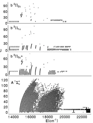
The new and old sources for the data used in this study are summarized in TableI. Below, we give additional details about the older published data and more extensive informa- tion about the new data. A representation of all the data is shown in Fig.1. Dots are plotted for the state that is calcu- lated to have the largest component in the DVR eigenvalue calculated for each experimental term value. Clearly, the pre- ponderance of the data is for the A¹⌺u

+ state, and there are gaps in the data for the b³⌸u state. By way of orientation, potentials for the states of interest are shown in Fig.2.

We have chosen to use the minimum of the X state as the zero of energy. The fitting procedures here use term values rather than combination differences except as noted in Sec.

III B.

When combining data from many sources into a global fit, one key question is the relative weight given each data set. Nominally, the weight for each data point is equal to 1 /␴^{2, where}␴ is the estimated uncertainty. Where possible, we have used the published experimental uncertainties.

However, comparisons of observations of the same term val- ues from different data sets and our own experience in cali- brating spectra with iodine lines have in several cases led to upward adjustment of these uncertainties.

TABLE I. Sources of the data used in the present work. The first number in parentheses after A or b denotes vibrational numbers, after the semicolon, the rotational quantum numbers. PW, present work; Abs. Spec., absorption spectroscopy; LS, laser spectroscopy; Mod. Pop. Spec., modulated population spectroscopy; LES, laser excitation specroscopy; Mod. Gain, modulated gain; Pol. Spec., polarization spectroscopy; AOTR, all-optical triple resonance; DR, double resonance; PFAOTR, perturbation-facilitated all-optical triple resonance; FT, Fourier transform; PFOODR, perturbation-facilitated optical-optical double resonance.

Authors Year Reference Levels obs’d Technique

1. Kusch and Hessel 1975 8 A共0–10兲 Photographic Abs. Spec.

2. Kaminsky et al. 1976 9and10 A共14–43兲 共113 lines兲 Mod. Pop. Spec.

3. Atkinson et al. 1982 12and13 b共17,21,25; 艋40兲 Mol. Beam LES

4. Shimizu and Shimizu 1983 14 b共8–17; 艋20兲 Mol. Beam LES

5. Ahmad-Bitar and Al-Ayash 1984 44 A共22,25; 艋26兲 Mol. Beam LES

6. Gerber and Möller 1985 45 A共v=68; 艋12;v=66–70;0兲 Mol. Beam 2-step LES

7. Effantin et al. and Babaky 1985 15and16 A共0–10;0–104兲 FT emission from共2兲¹⌺g+

8. Chawla and co-workers 1985 21and22 A共62–105;10,14兲 Mod. Gain Spec.

9. Li et al. 1987 46 A共26,34兲,b共28,34兲 Pol. Spec.

10. Katô et al. 1988 47 A共8兲,b共14兲 Pol. Spec.

11. Whang et al. 1992 18and19 b共0–7,32–57;3–18兲 PFAOTR

12. Wang 1991 48 A共44,48;10–14兲 AOTR

13. Ji 1995 49 24 A – b “window levels” PFOODR

14. Tiemann et al. 1996 23 A共88–185; 艋21兲 Mod. Beam 2-step LES

15. Krämer et al. 1997 50 b共0; 0–14兲 Mol. Beam LES

16. Zalicki et al. 1993 20 A共0–3;2–85兲;b共6–9兲 Mol. Beam LES

17. Li 1990 PW A共0–2,5,12,17,22兲,b共17,21兲 PFOODR

18. Li, Lyyra, and Ahmed 2006 PW A共0–43; even J艋16兲 DR Pol. Spec.

19. Ross 2006 PW A共0–31;0–125兲 FT Abs. Spec.

20. Qi, Bai, Ahmed, and Lyyra 2006 PW A共0–50;0–125兲 Pol. Spec.

A. Data previously published

Kusch and Hessel⁸ used a 9.3 m concave grating spec- trograph to study the Na₂A←X band system. Parameters for the A state were extracted by ignoring perturbed levels. Per- turbation shifts ofv = 0 and 1 rotational levels of the A state are displayed in a plot in Ref. 8. We have been told that Kusch discarded the raw spectral data shortly before he died.

From the Y_ij parameters and the plotted shifts, we recon- structed term values for A state v = 0 and 1 levels and used these estimates at an early stage of this study.

One of the prominent early achievements of laser spec- troscopy was the thesis⁹ of Kaminsky with Schawlow.

Modulated population spectroscopy¹⁰ was used to separate individual absorption lines from the dense spectral back- ground. 113 transitions are listed in Ref.9with A state quan- tum numbers ranging fromv = 14 to 43 and J values prima- rily 12, 14, 27, 29, 42, and 44. The quoted uncertainties of 0.03– 0.30 cm⁻¹ are relatively large, so the data were used only in the early phases of this study.

Direct observation of spin-forbidden transitions b³⌸u

←X¹⌺g

+was made possible by observing laser-induced fluo- rescence from a molecular beam.¹³ In the thesis of Atkinson,¹²data for the b-X共17,0兲, 共21,0兲, and 共25,0兲 bands, each with all three ⍀ components, are given for J values from 0 to 40.

A wider range of b state vibrational levels, fromv = 8 to 17共but with J艋20兲, was observed, also by molecular beam laser-induced fluorescence, by Shimizu and Shimizu.¹⁴ Al- though the quoted calibration uncertainty is 0.0015 cm⁻¹, comparisons of data on the same vibronic levels in the pre-

vious data set exhibited differences as large as 0.008 cm⁻¹. Therefore, each set was given a standard deviation ␴ ^of 0.005 cm⁻¹.

Ahmad-Bitar and Al-Ayash⁴⁴ reported observations of ten A←X bands by laser absorption of a supersonic molecu- lar beam, with 40 MHz linewidth. Unfortunately, line posi- tions were given only for the共25,3兲 and 共22,1兲 bands.

High vibrational levels 共v=66–70兲 of the A state were observed by Gerber and Möller using two-step excitation in separate interaction regions of a molecular beam.⁴⁵From the first region, excited A state levels decay to v

⬙

= 31 of the X state, which were reexcited. Here also, the published line measurements the共68,31兲 band are a regrettably small frac- tion of the total.

We have also been able to use a more extensive set of spectral line data from the work of Effantin et al.¹⁵ The A state was observed in emission from the共2兲¹⌺g

+state, which was populated by collisional transfer from the B¹⌸u state, which in turn was excited by several Ar⁺laser lines. The data cover the range 0艋v艋10 of the A state, with J艋104. We transcribed more than 5000 handwritten line measurements into electronic files. By comparison with term values ob- tained from A←X transitions, this data set yields apparent shifts of 0.01– 0.05 cm⁻¹, possibly due to collisional transfer from the level originally excited to another level from which fluorescence was observed.

In order to access higher levels of the A state, Chawla and co-workers^21,22used modulated gain spectroscopy. This involved excitation of v = 7 or 26 of the A state by a pump

FIG. 1. Summary of the data used in this study. The observed term values are sorted according to the largest component in the calculated eigenvector.

FIG. 2. Adiabatic potentials for Na₂ungerade states in the energy region of this study, obtained by diagonalizing the DVR matrix for J =兩⍀兩, for each value of R. Vibrational quantum numbers are shown for the A and b states.

The top plot shows the lower levels, with an inset showing the avoided crossing region. The bottom plot, also with an inset, shows levels and turn- ing points closer to the dissociation limit. Eigenvalue calculations, however, used diabatic potentials and spin-orbit coupling functions.

laser, and then decay in a resonant cavity to sparsely occu- pied v = 19 or 39, respectively, of the X state, thereby pro- ducing an “optically pumped laser共OPL兲.” Transitions to v

= 62– 105 levels of the A state were detected by their effect on the gain of the OPL. P / R doublets with J

⬙

= 11 were mea- sured to an accuracy of 0.006 cm⁻¹.

Li et al.⁴⁶used pump-probe techniques to selectively ob- serve certain A←X transitions. In particular, they studied perturbations between A共v=26兲 and b共v=28兲 and between A共v=34兲 and b共v=34兲. Although a heat pipe oven was used, the geometry of the pump-probe technique reduced the line- width to a residual linewidth of 25 MHz.

At about the same time, Katô et al.⁴⁷ used Doppler free polarization spectroscopy to study the perturbative interac- tions between A共v=8兲 and b共v=14兲. Resolved hyperfine structure was also reported in this work.

Whang et al.^18,19used perturbation-facilitated all-optical triple resonance 共PFAOTR兲 to observe a large number of levels of the b state. A level of the A state mixed with the triplet b was the first excitation step, followed by excitation to a level of the 2³⌸g state, and then stimulated decay to b state levels. Various rotational levels 3艋J艋18 with v

= 0 – 7 and 32–57 of the b state were observed by monitoring fluorescence of the 2³⌸gstate. The cumulative measurement uncertainty from these multiple steps was estimated to be 0.01 cm⁻¹.

Another AOTR scheme was used by Wang⁴⁸ to excite moderately high levels of the A state. Low levels of the A state were first excited from the X state, followed by stimu- lated decay to high levels of the X state, and reexcitation to higher levels of the A state. Levels with J = 10, 12, or 14 for v = 44– 48 and 55–61 were observed, with uncertainties esti- mated to be 0.02 cm⁻¹.⁴⁸

As part of a thesis on long-range potentials in K₂ and Na₂, Ji⁴⁹used singlet-triplet A⬃b levels as window states to access higher triplet states. This thesis lists 24 such mixed levels that were observed in the course of a study of the Na₂ 共1兲 ³⌬gstate.

Tiemann et al.²³were able to excite levels of the A state up to the dissociation limit by Franck-Condon pumping from v = 0 to v = 27 or 31 of the X state via v = 13 of the A state, followed by excitation with a second laser tov = 88– 185 of the A state. Because of a high degree of collimation of the molecular beam, the residual Doppler width was only 5 MHz. Experimental uncertainties mostly vary between 0.0003 and 0.030 cm⁻¹, but in a few cases from overview spectra recorded with a multimode laser, they amount to 0.15 cm⁻¹.

Krämer et al.⁵⁰used a beam of Na₂molecules to directly excite the intercombination transition from X共v=0兲 to b共v

= 0兲. ⍀=0 and 1 components of the b state were observed up to J = 14, with a calibration accuracy of 0.015 cm⁻¹.

B. Unpublished data

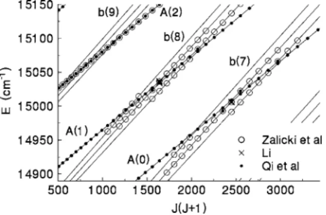
Laser spectroscopy with a molecular beam. Zalicki et al.²⁰ in 1993 at Laboratoire de Spectroscopie Hertzienne de l’ENS and at the Université Pierre Marie Curie, Paris, used a supersonic beam of Na₂ molecules and a ring dye laser to

excite v = 0 – 3 of the A state to study perturbations with v

= 6 – 9 of the b state. The spectral linewidth was typically greater than 40 MHz 共the residual Doppler width兲, as many transitions were power broadened to increase the detection sensitivity for transitions that were predominantly b←X character. 392 term values, 2艋J艋85, from these observa- tions are included in the present data set. Calibration was with a wave-meter and iodine reference lines. For levels with appreciable triplet character, the hyperfine structure was well resolved. For this study, the hyperfine center of gravity was taken as the effective line center. The rotational populations of ground state levels were studied in a separate work.⁵¹

Perturbation-facilitated optical-optical double reso- nance spectroscopy. This technique was used especially to measure mixed singlet-triplet states for use as window states to excite higher triplet levels. 117 levels were excited over a wide range of energies by one of us 关Li; data obtained at MIT 共1982–1984兲, University of Iowa 共1987–1989兲, and Temple University共1993–2001兲兴.

Optical-optical double resonance polarization spectros- copy. This technique was used earlier in this study 共at the University of Iowa in 1990, by Li and Lyyra, with calibra- tions verified later by Ahmed兲 to obtain data on 544 A state levels up to v = 44, even with J values 艋16. The “V-type”

polarization scheme has been described in Refs. 52 and53 and differs from the technique described below in that the pump laser excited a different upper state than the probe laser. For other examples of this technique as applied to higher electronic states of Na₂, see Refs.54and55.

Absorption spectroscopy. A Doppler-limited absorption spectrum of Na₂was recorded共by Ross, in Lyon兲 on a Fou- rier transform spectrometer at an instrumental resolution of 0.02 cm⁻¹, in part to replace the lost original data of Ref.8.

Na₂ molecules were formed in a short 共20 cm兲 heat pipe oven, operated at 480 ° C with argon as a buffer gas. Mea- sured widths共full width at half maximum兲 of isolated lines were Doppler limited 共0.05 cm⁻¹ at 17 200 cm⁻¹兲. Instru- mental calibration was checked by recording the absorption spectrum of I₂ with the same optical alignment. Nearly 10 000 lines were measured over the range 13 300– 17 200 cm⁻¹. At the high energy end, line assign- ments were complicated by extensive overlapping due to the Doppler linewidths. Polarization spectroscopy eventually provided data at higher resolution, so the absorption spectra data were not actually included in the final fit.

Polarization spectroscopy. Extensive new measurements of Na₂A←X transitions have been performed 共by Qi, Lyyra, and Bai兲 at Temple University using the technique of polar- ization spectroscopy.²⁴ This technique was first used to ob- serve hyperfine structure in the hydrogen atom Balmer-␤ transition,⁵⁶and more recently, it has been used in molecular spectroscopy studies.^36,52,57 The basic principles are clearly discussed in Refs.52and58and will be reviewed here very briefly.

For polarization spectroscopy, a linearly polarized single mode tunable laser beam is split into a weak probe beam and a pump beam 共see Fig.3兲. The stronger pump beam passes through a␭/4 wave plate and becomes a circular polarized beam 共either left handed or right handed兲. The probe beam

passes through a polarizer, the molecular sample, and an ana- lyzer, a polarizer crossed with the first one. The linearly po- larized probe beam and the pump beam counter-propagate.

The sample is isotropic without the pump beam and the de- tector only receives a very small residual signal from imper- fectly crossed polarizers or some birefringence of the cell windows.

The pump is absorbed by the molecular sample when the optical frequency is tuned to a molecular transition, which we write as 共J

⬘

^{, M}

⬘

^兲←共J

⬙

^{, M}

⬙

兲, where M denotes the mag- netic quantum number referred to an axis along the direction of beam propagation. In zero external field, the M compo- nents are degenerate and equally populated. However, the transition amplitudes for the pump beam vary with M, and thus certain magnetic sublevels are partially depleted by the pump beam. For this reason, the originally isotropic molecu- lar sample becomes anisotropic in the presence of the pump beam. When the probe beam passes through the anisotropic molecular sample, each circular component will experience a different phase shift and also a differential absorption. From both effects, there will be a signal through the crossed polar- izers, provided that the pump and probe beams interact with the same molecules. Since they are traveling in opposite di- rections, this implies that the affected molecules will be those with negligible Doppler shift; hence, this makes sub- Doppler width spectroscopy possible.

As discussed in Refs.24,52, and58, the resultant signal has Lorentzian and dispersion components. The orientation of the analyzer prism can be adjusted to null out the disper-

sion term and maximize the Lorentzian term. Figure4shows part of a typical scan together with the I₂ laser excitation spectroscopy 共LES兲 signal, the Vernier étalon 共VET兲 chan- nel, which is used to monitor mode hops during the laser scans, and a LES signal also from Na₂, exhibiting a Doppler linewidth. Mode hops appear as discontinuities in the VET scan. Each 1 cm⁻¹ segment consists of three 10 GHz con- tinuous scans and the joints of these segments introduce some uncertainty into the calibration. Iodine lines within each 10 GHz segment are used for calibration of that seg- ment. When no calibration lines appeared in a 10 GHz seg- ment, interpolation between adjacent segments was required.

The calibration procedure was based on the Doppler-limited iodine atlas,⁵⁹with corrections from Ref.60and later by Ref.

61. Overall, the mean calibration uncertainty was estimated to be 0.005 cm⁻¹. The heat pipe oven temperature for these experiments was 570 K.

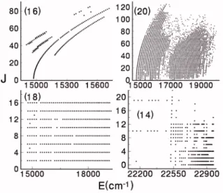
Figure5 shows the range in energy and rotational quan- tum number for four of the unpublished data sets listed above. In other cases, the range is clear from the discussion or the publication.

In each case where term values are calculated from ex- perimental lines, the Na₂X state Yij parameters of Ref.62 共data set II兲 共hereafter referred to as KHII兲 have been used. A value of Y₀₀= −0.031 77 cm⁻¹ for the X state is obtained from these Y_ijvalues. The G共v兲 values given by Ref.63, and from combination differences obtained from the lines mea- sured by Ref. 24, agree with the KHII values within 0.006 cm⁻¹. However, recent measurements cited in Refs.23 and64give energies of X state levels J = 0,v = 27 and 31 that are smaller than predictions from KHII by 0.0197共44兲 and 0.0170共37兲 cm⁻¹, respectively. The term values from Refs.

21 and 45 have been adjusted accordingly. In general, one can say that the accuracy of A and b state level energies presently is tied to both the wavelength calibration accuracy and the accuracy of the energies of the X state. Further im- provement might require an alternative calibration technique, such as frequency combs.

FIG. 3. A schematic of the experimental setup for polarization spectroscopy.

Lateral detection of the total fluorescence records a Doppler-limited laser excitation spectrum.

FIG. 4. A typical region of the polarization spectrum showing 共top兲 the vernier etalon signal共VET兲 signal used to check that the laser scans con- tinuously,共middle兲 the I2LES signal for calibration,共bottom兲 the Doppler- limited Na₂LES signal, and the Na₂polarization spectroscopy signal, which exhibits a sub-Doppler width.

FIG. 5. The range of the data for the Na₂A and b states from several of the individual data sets. The numbers in parentheses refer to the data source numbers listed in the first column of TableI.

The dissociation limit D₀of the X state to the free atom hyperfine center of gravity共hfs cog兲 has been accurately de- termined by Ref.64 to be D₀= 5942.6880共49兲 cm⁻¹. In this work, energies are referenced to the minimum of the X state, which lies 79.3426 cm⁻¹ below v = 0, as obtained from the Yij parameters of KHII and Y₀₀given above. From Ref. 65, the transition energy from hfs cog energies of a 3²S atom to a 3²P_1/2 atom is 16 956.170 27共4兲 cm⁻¹. From the 3²P_1/2 cog to the cog of the 3³P state, it is 11.4639 cm⁻¹ 关共2/3兲⌬atom= 17.1959 cm⁻¹兴. Since spin-orbit structure is considered here, the relevant quantity is thus a dissociation limit of 22989.6648 cm⁻¹. Technically, the threshold for free

2S共F=1兲+²P_1/2共F=1兲 atoms lies at a limit of 22 978.1599 cm⁻¹. However, we have found that the experi- mental data extrapolate essentially to the hfs cog, which has a limiting value of 22 978.2009 cm⁻¹and is consistent with the 3²S + 3²P fine structure cog of 22 989.6648 cm⁻¹ as given above. Although the experimental data from Ref. 23 extend to v = 185, only data to 22 978.05 cm⁻¹ 共slightly abovev = 177 as shown in Fig.2兲 were included in the analy- sis to avoid hyperfine structure effects, which are not in- cluded in the present model, but were of primary concern in Ref.23.

For absorption spectroscopy or single-photon polariza- tion spectroscopy, the range of accessible upper state levels is limited by the transition strengths, which are determined by the vibrational overlap factor including the A-X electronic transition dipole moment具A共v

⬘

^{兲兩␮共AX兲兩X共v}

⬙

兲典, and the Bolt- zmann thermal factor for the X state level. The electronic transition dipole moment function is obtained from ab initio psuedopotential calculations and confirmed by experiments in Ref. 66. Results are plotted in Fig. 6. We have calculat- ed the line strengths using a Boltzmann factor, exp关−E共v

⬙

^{, J}

⬙

^兲/kBT兴, and the A-X electronic transition dipole moment function, 具A共v

⬘

^兲兩␮共AX兲兩X共v

⬙

兲典, obtained from pseudopotential ab initio calculations and confirmed by ex- periments by Ref.66. Results are plotted in Fig.6.

III. FITTED POTENTIALS AND SPIN-ORBIT FUNCTIONS

A. Molecular Hamiltonian

This study of interactions between the A¹⌺u

+and b³⌸u

states of Na₂is limited to levels of parity共−1兲^J, e symmetry, by selection rules. We will not address hyperfine structure effects and therefore ⌬J=1 hfs couplings with f symmetry levels, parity −共−1兲^J, and⌬J=0 hfs couplings between g and u states will not be not considered.

The molecular Hamiltonian⁶⁷ includes elements for 共ra- dial兲 kinetic energy HK, nuclear rotation H_rot, and potential energy including spin-orbit effects H_V:

H共R兲 = HK+ H_V共R兲 + Hrot共R兲, 共1兲 where R is the internuclear distance. Spin-orbit functions are discussed in Sec. III D. Since the present data extend to very near the dissociation limit, we use forms for the rotational energies that are transformed to case a from the case e ex- pressions, as in Ref.68. Hence, G共v兲 values may differ from other conventions. For this reason, in presentations below,

we will refer to our vibrational energies with the notation G˜ 共v兲, which translates to the usual convention for¹⌺u+states as G共v兲=G˜ 共v兲+2Be共see, for example, TableIV兲. For e sym- metry levels, the nonzero matrix elements of H_V共R兲 + H_rot共R兲 are

具¹⌺⁺兩H兩¹⌺⁺典 = V共¹⌺⁺兲 + 共x + 2兲B,

具³⌸_⍀兩H兩³⌸_⍀典 = V共³⌸兲 + 共⍀ − 1兲⌬d+共x + 2⑀兲B,

具¹⌺⁺兩H兩³⌸₀⁺典 = − ⌬od, 共2兲

具³⌸₀兩H兩³⌸₁典 = −

冑

2xB, 具³⌸₁兩H兩³⌸₂典 = −

冑

2共x − 2兲B,

where x = J共J+1兲, ⑀^{= 1}共for ⍀=0 and 1兲 and −1 共for ⍀=2兲, and H^†= H. In the above, V共¹⌺u

+兲, V共³⌸u兲, ⌬d, ⌬od, and B

= B共R兲=ប²/ 2␮^R2共1/100hc兲 are functions of R 共␮^{is the re-} duced mass兲. 共Here␮^{, R,}ប, and c are in SI units, and all V,

⌬, and B quantities are in cm⁻¹. The factor 1 / 100hc converts from SI units to conventional spectroscopic cm⁻¹.兲 ⌬d and

⌬od are diagonal and off-diagonal spin-orbit functions, re- spectively.

For test purposes, we also preformed six-channel calcu- lations using additional Hamiltonian elements for the B共1兲¹⌸u and共2兲³⌺u state plus coupling elements between these states and those represented in Eq.共2兲. Such elements are given in Refs.67and68. Since the R dependence of the additional spin-orbit functions and L-uncoupling functions is not known, we took these functions to be constant with the value appropriate for the asymptotic limit. These additional elements are needed to produce exact convergence to the 3²S + 3²P center-of-gravity limit without spin-orbit func- tions, or to the P_1/2and P_3/2limits with spin-orbit functions, as shown in Fig.2, for which the potentials are obtained by diagonalization of the DVR matrix at each R value 共for J

=兩⍀兩兲. Although the Hamiltonian matrix elements in Eq.共2兲 by themselves do not converge to the correct limit, we found that up tov = 177 of the A state, the difference in eigenener- gies between four- and six-channel calculations was no more

FIG. 6. This plot shows relative band intensities, calculated from the prod- uct of the vibrational overlap,兩具A共v⬘兲兩␮共AX兲兩X共v⬙兲典兩², including the A←X transition moment from Ref. 66, times the Boltzmann factor, exp关−E共v⬙^{, J}⬙兲/kT兴. Here, T=600 K, J⬙^{= 30.}

than 3 MHz. Hence, given the present limited objectives, four-channel calculations are deemed sufficient.

The DVR Hamiltonian matrix has a dimension equal to the number of R mesh points, i, times the number of chan- nels 共¹⌺u+, ³⌸_0u, etc.兲, j 共艋4 in the present approximation兲.

The elements in Eq. 共2兲 are diagonal in i but may be off- diagonal in j. Since all mesh points are used in calculating d²/ dR²,³¹the kinetic energy共a full matrix over i兲 is obtained as accurately as possible. As in Ref. 35, scaling is used to make the mesh points more dense where the momentum can be greatest, namely, for R values near minima of the poten- tials. The eigenfunctions obtained by diagonalizing the DVR matrix give the wave function components in each channel.

The eigenvalues include effects of mixing between different channels, including the continua. Hence, this approach is a powerful alternative to calculating vibronic coupling ele- ments with wave functions obtained by the Numerov method, but does require diagonalization of a fairly large matrix for each J value. Applying the DVR method, experi- mental term values are used to fit potential and spin-orbit function parameters. Accurate term values for perturbed lev- els can be obtained only by solving the DVR eigenvalue problem for the coupled states, or from tables, as given in the EPAPS files.⁴³

B. The fitting process

As stated above, in this study there were several stages in fitting the data to potential and spin-orbit parameters as more detailed data were obtained. At each stage, intensities were estimated from calculated A-X Franck-Condon factors, rotational line strengths, and the X state Boltzmann factor for the experimental temperatures. The new polarization spec- troscopy lines were matched with calculated line positions to successively smaller tolerances, ultimately 0.02 cm⁻¹. All term values calculated from these lines 共by adding ground state energies兲 were given a ␴ 共uncertainty兲 of 0.005 cm⁻¹. Values for ␴ varied between 0.002 and 0.02 cm⁻¹ for the other data sets.

We used 24共12兲 nonzero short-range potential param- eters for the A共b兲 state, 4 long-range potential parameters for each, and spin-orbit parameters as discussed below. Nor- mally, not more than 15 parameters were varied simulta- neously, but from iteration to iteration, the parameter set was traversed several times. For levels up to 10 cm⁻¹ below the dissociation limit, it was sufficient to carry the DVR mesh points in R out to 40 Å, with 320 mesh points in R, giving a 1280⫻1280 DVR Hamiltonian matrix for four-channel cal- culations for each J艌2. For levels closer to the dissociation limit, as many as 1500 mesh points out to R = 150 Å were used, but these cases involved only J values艋22.

Some of the data from Ref.23with the smallest experi- mental uncertainties, including data close to the 3S + 3P_1/2 dissociation limit, were in the form of difference frequencies.

Four-channel calculations using our fitted parameter set re- produced these difference frequencies to within 20 MHz, ex- cept for a few outliers and also data from levels within 1 cm⁻¹of the P_1/2dissociation limit, where evident hyperfine

effects increased the residuals to as much as 150 MHz. A detailed study of the regime very near the dissociation limit is beyond the scope of the present work.

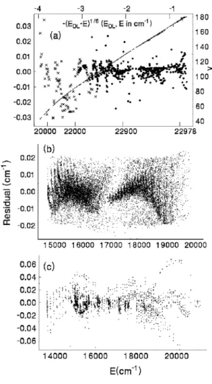
The overall variance of the fit of A / b data within the present data set to potential and spin-orbit parameters was 2.85, after many iterations. To indicate the quality of the fit, we plot in Fig.7共a兲the residuals from the two data sets at the highest energy, in Fig.7共b兲the residuals from the new polar- ization spectroscopy data, and in Fig. 7共c兲the residuals for the other data sets. The final rms residual for the former was 0.0080 cm⁻¹ 共240 MHz兲. Combination differences for the X state from this data set agreed with E共v,J兲 values calculated from the Yijparameters of KHII共Ref.8兲 to a rms residual of 0.006 cm⁻¹.

From the residuals plotted in Fig.7, it does appear that couplings with states outside the Hamiltonian basis may pro- duce small J-dependent shifts. The most likely culprits are the B¹⌸ustate coupling with the A¹⌺u+ state and the a³⌺u+

state coupling with the b³⌸ulevels. We did attempt to intro- duce A⬃B L-uncoupling terms into a larger Hamiltonian matrix, but the results were not decisive, and in any case, the

FIG. 7. Residuals from共a兲 the data from Refs.23共dots兲 and21共crosses兲, 共b兲 the new polarization spectroscopy data, and 共c兲 all other data sets in- cluded in the fit. The energy in共a兲 is scaled as 共EDL− E兲^1/6to expand the region near the dissociation limit, E_DL= 22 978.2009 cm⁻¹, so as to show systematic effects due to hyperfine structure above E = 22 978 cm⁻¹. Vibra- tional quantum numbers共smaller dots in a nearly straight line兲 are plotted with reference to the right axis. Data for 共b兲 were selected to be within 0.02 cm⁻¹of the energy calculated from the fitted parameters.

R dependence of such elements is not known. Therefore, all results quoted here are from the four-channel Hamiltonian matrix, as stated above.

C. The potential functions

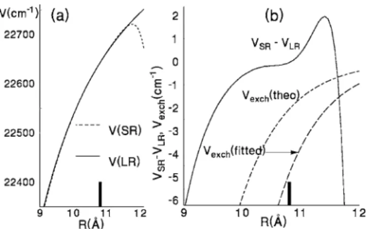
The Born-Oppenheimer potential functions are divided into short-range and long-range regions. The long-range po- tential for the A state is composed of the exchange potential and dispersion terms: V_LR共R兲=Vexch+ V_disp. Typically, the transition point RTis chosen to be comparable to the Le Roy radius,⁶⁹ R_LR, which indicates approximately the R value at which the atomic wave function overlap becomes negligible, and the expansion in inverse powers of R becomes valid. The original estimate⁶⁹ from atomic radii, R_LR= 2关具r²典A

1/2

+具r²典B1/2兴, was found to be inadequate for excited states, and an m-dependent expression was introduced in Ref. 70:

R_LR-m= 2

冑

3关具nlm兩z²兩nlm典A

1/2+具n

⬘

^l

⬘

^m

⬘

兩z²兩n

⬘

^l

⬘

^m

⬘

典B

1/2兴, to repre- sent the orientation of the atomic orbitals. Here, n and n

⬘

^are principal quantum numbers, l and l

⬘

are the atomic electronic orbital angular momenta, and m and m

⬘

are the components of l and l

⬘

along the internuclear axis for the outermost elec- trons. For Na₂ 3s_␴+ 3p_␴ and 3s_␴+ 3p_␲, the values of R_LR-m from Ref.70are 13.4 and 9.7 Å, respectively. There are no experimental b state term values above 20 700 cm⁻¹, corre- sponding to an outer turning point of 5.75 Å, so there is no direct information on the long-range part of the potential for the b state. However, as the available data on the A state extends to nearly the dissociation limit, it is possible to ex- tract information on both the long-range coefficients and the exchange potential for this state.

For the short-range region, R艋RT, we use the analytic expression adopted by the Hannover group,^27,28

V_SR共R兲 =

兺

i=0 I

ai

冉

^{R + bRR − RM}M

冊

^{i. 共3兲}

In this work, we typically set a₁= 0, so that RM= Re, the R value at the potential minimum, and thus a₀= Te. The param- eter b was adjusted to achieve an optimum fit with a mini- mum number of parameters. The advantage of this param- etrization as compared with the traditional Dunham/RKR approach is that the semiclassical approximation does not enter, and the divergence at large R is less of a problem, since V_SR共R→⬁兲=兺iaiis finite共though extremely large兲.

Note that if a₁= 0 in Eq.共3兲, then it follows that

⳵^2V

⳵^{R2共R = Re兲 =} 2a₂ R_e²共1 + b兲²;

⇒␻e= 1

10␲共1 + b兲Re

冉

^2ha␮^2c

冊

^{1/2, 共4兲}

where␮is the reduced mass.␮, h, c, and Reare in SI units, while a₂and␻eare in cm⁻¹. The potential parameters aifor the A¹⌺u

+and b³⌸ustates are listed in TableII. Fitted values for Te,␻e, and Reare given in TableIII. As stated above, for purposes of comparisons in TableIII, we present our results in the form Te= T˜

e+ 2Befor the A state and Te= T˜

e+ Befor the b state. Term values calculated with the A state parameters of Ref. 8 give v = 0 term values about 0.06 cm⁻¹ higher than

observed in the present work. Results from Refs. 20and24 and from absorption spectroscopy in Lyon agree to within less than 0.01 cm⁻¹, suggesting a 0.06 cm⁻¹calibration error in the earlier work of Ref.8. The remaining difference in the A state values for T_eis due to perturbation shifts that were not analyzed in Ref. 8. In TableIII, the uncertainties for T_e and ␻e are determined primarily by wavelength calibration uncertainties. Note that the uncertainties for R_evalues reflect a range of rotational energies spanning 500– 1000 cm⁻¹, and that centrifugal distortion effects are determined by the po- tential function rather than by additional parameters. How- ever, L-uncoupling interactions with states outside the four- channel Hamiltonian matrix and also possible sensitivity to the form of the potential are not included in the estimates of the uncertainty of the Revalues.

The exchange interaction for a ¹⌺u+ state from 3s + 3p atoms, as given by Bouty et al.⁷¹共see also Refs.72and73兲, is

V_exch= q关I共310,300兩310,300兲 + I共310,300兩300,310兲兴, 共5兲 where q is an amplitude factor that was adjusted in the fitting process. The two integrals, I共n1, l₁, m₁, n₁

⬘

^{, l}1

⬘

^{, m}1

⬘

兩n2, l₂, m₂, n₂

⬘

^{, l}2

⬘

^{, m}2

⬘

兲, represent ex- change with and without excitation transfer.⁷¹ Each includes a factor共A3sA_3p兲²which is uncertain to some degree, so it is considered appropriate to adjust q 关the quotient, optimized value/ab initio value, of共A3sA_3p兲²兴 in the fitting process.⁷⁴

The dispersion terms in V_LRare given by

TABLE II. Fitted parameters for the V_SRpotential function, for the A and b states. Te= a₀and Reare given in the following table. a₁= 0. The aiare in cm⁻¹, while b is dimensionless. Numbers in square brackets denote the power of 10. For the A state, R艋2.357 Å, the form V=A/R⁴+ C applies, with values given below.

A state b state

b 1.692 142 646 0.230

a₂ 2.252 672 639 84关5兴 5.928 917 446 45关4兴 a₃ −6.999 292 760 99关5兴 −2.244 248 711 459关3兴 a₄ 9.633 810 729 92关5兴 −6.676 242 575 792关4兴 a₅ 9.050 944 761 15关5兴 −9.877 399 975 864关5兴 a₆ −1.353 816 744 09关7兴 1.990 153 164 054关5兴 a₇ 1.968 679 893 00关7兴 5.521 114 946 502关5兴 a₈ 1.778 001 698 55关8兴 −2.169 520 362 189关6兴 a₉ −1.245 607 952 89关9兴 −2.884 323 344 369关6兴 a₁₀ 2.193 078 450 59关9兴 8.119 353 310 882关6兴 a₁₁ 2.802 520 057 56关10兴 4.259 151 884 120关5兴 a₁₂ −2.397 623 078 49关11兴

a₁₃ 6.090 618 458 01关11兴 A state, R艋2.357 Å:

a₁₄ 6.476 255 150 53关11兴 V共R兲=A/R⁴+ C;

a₁₅ −4.752 613 018 90关12兴 A = 7.187 53关5兴 cm⁻¹Å⁴ a₁₆ −2.489 570 504 02关12兴 C = 2.457 835 9关3兴 cm⁻¹ a₁₇ 4.002 905 840 06关13兴

a₁₈ −4.334 056 442 24关13兴 a₁₉ −1.837 113 429 17关14兴 a₂₀ 8.301 971 726 55关14兴 a₂₁ −1.704 450 623 24关15兴 a₂₂ 1.883 672 875 43关15兴 a₂₃ −8.737 759 108 58关14兴