基於深度學習語義分割之城市道路汽車轉向操控

(1)

國立臺灣大學電機資訊學院資訊工程學系碩士論文

Department of Computer Science and Information Engineering College of Electrical Engineering and Computer Science

National Taiwan University Master Thesis

基於深度學習語義分割之城市道路汽車轉向操控

A Deep Learning Based Semantic Segmentation Approach for Car Steering on Urban Roads

塗國星 Kuo-Hsin Tu

指導教授：傅立成博士共同指導：蕭培墉博士 Advisor: Li-Chen Fu, Ph.D., Pei-Yung Hsiao, Ph.D.

中華民國 106 年 7 月

July 2017

(2)

口試委員會審定書

(3)

誌謝

能完成這篇論文，我要特別感謝我的指導教授傅立成老師與共同指導的蕭培墉老師，也要感謝實驗室的宗穎，學弟翔宇和興宇在計畫案的協助，特別感謝同樣來自中央的學弟翔宇和禹齊在最後的時刻支援碩論的實驗，讓我可以沒有後顧之憂，持續完成論文的進度。另外，也感謝在各課程中認識的同學，透過一起合作課程專題，讓我們認識彼此互相鼓勵，在台大能認識各位一切都是緣分。其實這次能進入台大就讀研究所，過程實屬不易，在忙碌的科技產業工作同時準備學校的申請與考試，是個蠻大的挑戰，最後能夠順利就讀台灣第一學府，真的是個恩典。在這段求學的過程，也是個挑戰，因為工作了一段時間，離開學校的環境蠻長一段時間，回到學校念書需要許多調適，特別是與台灣頂尖的人才一起修課，

互相競爭，當中壓力也不小，因此我也要感謝在過程中所有支持、鼓勵我的人，

願你們在各樣事上都能蒙福。最後，我要感謝我的父母，在這段期間成為我的後盾，透過各樣的方式支持與幫助我，使我能走到最後。

將一切頌讚、榮耀、感謝都歸於我在天上的父！

塗國星僅誌於國立台灣大學資訊工程研究所智慧型機器人與自動化實驗室 2017 年 7 月 28 日

(4)

中文摘要

在視覺式自動駕駛系統中，感知與控制是兩個重要且待解決的議題。此外，

由於深度卷積神經網路在解決感知與控制問題上有非常好能力，使得深度卷積神經網路成為視覺式自動駕駛系統的解決方案之一。在本論文中，我們證明語義分割可以用來提升視覺式自動駕駛系統的效能。論文中提出了一個使用語義感知並基於端對端深度卷積神經網路的方法來解決自動駕駛中的視覺式控制問題。所提出的方法具有兩個階段並透過影像輸入來預測汽車轉向操控。在第一個階段中，

使用一個深度卷積神經網路從輸入影像產生語義分割的結果，在第二個階段中則使用另一個深度卷積神經網路從語義分割資訊來預測出汽車轉向操控。在實驗中，我們使用一個公開的汽車駕駛資料集來評估所提出的方法，實驗結果顯示該方法能達到比一般端對端的深度卷積神經網路方法更好的結果。

關鍵字：深度學習、卷積神經網路、語義分割、自動駕駛、車輛轉向

(5)

Abstract

In vision based autonomous driving systems, perception and control tasks are two critical problems to be solved. The effectiveness of deep convolutional neural networks (CNNs) in solving visual perception and control tasks has made CNNs a desirable solution for autonomous driving. In this thesis, we show that semantic segmentation can be applied to enhance the performance of a vision based autonomous driving system.

We propose an end-to-end CNN architecture with semantic perception to solve the vision based control problem in autonomous driving. The proposed approach is a two-stage CNN architecture that takes a monocular image and outputs a steering angle.

In the first stage, a CNN module is used to generate semantic segmentation from the input image. In the second stage, another CNN module is used to take advantage of the semantic perception to predict steering angles. In the experiment, a publicly available dataset of human driving data is used to evaluate the proposed method. Experimental results demonstrate that the proposed method enhance the results of the typical end-to-end CNN approach.

Keywords: Deep learning, Convolutional neural networks, Semantic segmentation, Autonomous driving, Vehicle steering

(6)

List of Figures

Figure 1-1: End-to-end CNN approach for steering control... 2

Figure 1-2: A two-stage CNN architecture. ... 2

Figure 2-1: Three main modules for an autonomous driving system. ... 9

Figure 2-2: Imitation learning in the context of steering control. ... 10

Figure 2-3: Paradigm of transfer learning. ... 12

Figure 2-4: A convolutional layer arranges its neurons in three dimensions... 13

Figure 2-5: A filter is used to produce a new feature map. ... 14

Figure 2-6: Local connectivity of a convolutional layer. ... 15

Figure 2-7: Illustration of the max pooling operation. ... 16

Figure 2-8: Illustration of a fully connected layer. ... 16

Figure 2-9: Plots for various non-linear activation functions. ... 17

Figure 2-10: Architecture of VGG-16. ... 18

Figure 2-11: Comparison of different vision problems. ... 19

Figure 3-1: System architecture of the proposed approach. ... 23

Figure 3-2: Architecture of the Perception Network. ... 25

Figure 3-3: Architecture of the encoder network... 26

Figure 3-4: Illustration of max-pooling indices. ... 27

Figure 3-5: Architecture of the decoder network... 28

Figure 3-6: Illustration of the decoding process. ... 29

Figure 3-7: Overview of the second stage. ... 30

Figure 3-8: Architecture of the Control Network. ... 31

Figure 4-1: Example images and annotations from the Cityscapes dataset. ... 36

(9)

Figure 4-2: Example images from the Udacity Self-Driving Car Dataset. ... 37

Figure 4-3: Absolute errors of the baseline model across the test data. ... 42

Figure 4-4: Absolute errors of the proposed model across the test data. ... 43

Figure 4-5: An image from error case #1 (frame 1857). ... 46

Figure 4-6: Prediction results of error case #1. ... 46

Figure 4-7: Comparison between feature maps from different models (frame 1857). .... 47

Figure 4-8: Result of semantic segmentation for frame 1857. ... 48

Figure 4-9: Semantic meaning and the corresponding color ... 48

Figure 4-10: An image from error case 2 (frame 4400). ... 49

Figure 4-11: Prediction results of error case #2... 49

Figure 4-12: Comparison between feature maps from different models (frame 4400) ... 50

Figure 4-13: Result of semantic segmentation for frame 4400 ... 51

Figure 4-14: An image from error case #3 (frame 918). ... 51

Figure 4-15: Prediction results of error case #3. ... 52

Figure 4-16: Result of semantic segmentation for frame 918. ... 52

Figure 4-17: Comparison between feature maps from different models (frame 918). .... 53

Figure 4-18: Sample segmentation results for the test set. ... 55

(10)

List of Tables

Table 4-1: Hardware specification for the experiment. ... 34

Table 4-2: Result on the test set of Udacity dataset. ... 41

Table 4-3: Results on the Udacity Self-Driving Car Challenge 2 leaderboard... 41

Table 4-4: Mean absolute errors and standard deviations for all error cases. ... 44

Table 4-5: Results of different segmentation model on the test set. ... 54

(11)

Chapter 1 Introduction

1.1 Motivation

In recent years, the development of autonomous driving is fast advancing. Car vendors and technology companies are moving forward to developing autonomous driving cars. One of the reasons is that autonomous driving cars can benefit humanity.

First of all, autonomous driving cars can provide us with more safety. According to a report from World Health Organization (WHO), nearly 1.25 million people die in road accidents each year [1]. Cars that drive by itself could reduce casualties in car accidents by making quicker and more stable decisions. Autonomous driving cars also improves the efficiency of transportation, which may lower global CO2 emissions and decrease the impact on global warming.

The idea of autonomous driving has been researched from 1930s. In the early days, these autonomous cars required human guidance and did not involve any intelligence.

Since 1980, truly autonomous driving technologies are invented, Ernst Dickmanns and his group at Bundeswehr University Munich built the world's first real autonomous driving car VaMoRs. Artificial intelligence for autonomous driving started to get people’s attention in 2005 DARPA Grand Challenge. Since then, research organizations have started to develop autonomous driving technologies, and in 2013 many major automotive manufacturers start to test autonomous driving systems.

Recently, numerous types of sensor are installed on an autonomous driving car to provide better and reliable perceptional functionalities. Common sensors can be found on an autonomous driving car are ultrasound, radar, LIDAR (Light Detection And

(12)

Ranging), and camera [2]. Among these sensors, visual sensors such as cameras can provide more information about the environment surrounding a car, for example, the color, texture, and appearance of objects can hardly be analyzed by others type of sensors. In addition, the infrastructures of urban roads have been built to be perceived by human vision, and naturally, it is important to research on vision based technologies so as to help autonomous driving cars perceive the world.

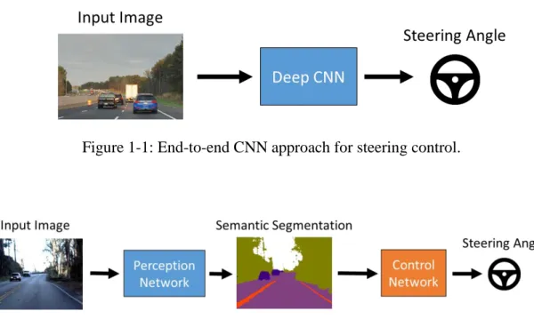
In recent years, the effectiveness of deep convolutional neural networks (CNNs) has been shown in various visual perception tasks such as object detection, object recognition, and semantic segmentation [3-6]. Besides, learning control policies from visual perception through CNNs has been proved promising [7, 8]. The recent research from NVIDIA also demonstrated an end-to-end CNN approach that could predict car steering from a monocular RGB image [9] (Figure 1-1). However, it is strongly believed that for robust steering control in autonomous driving, a higher level interpretation of the perceived scene will be extremely helpful.

Figure 1-1: End-to-end CNN approach for steering control.

Figure 1-2: A two-stage CNN architecture.

(13)

However, simply utilizing a raw RGB image for scene understanding would have a lot of noisy information that are not necessarily related to the scenario of driving. In general, we only need to focus on important objects in the scene and ignore unimportant details. For example, we only need to know where cars, pedestrians, and roads are located in the image and the overall layout of the scene. Actually, the visual processing of the human brain does perform information filtering. Generally, human visual perception has two sequential stages [10]. The first stage is pre-attentive stage, which processes all the information fast but coarsely, whereas the second attention stage processes part of the input information with more efforts. Note that pre-attentive processing accumulates information from the environment subconsciously. Information from the environment is pre-processed through pre-attentive processing. Then, our brain filters unimportant information and only continues to processes what is important [10].

Also, human beings have a remarkable ability to organize visual inputs. Instead of a bunch of intensity values, we perceive a number of visual groups, usually associated with objects. The visual system of human beings segments the visual input, which partitions the visual input into regions that have similar properties or semantic meaning.

This representation facilitates visual reasoning at the level of regions and their boundaries while not caring too much about the small details in the visual input [11].

Inspired by the visual processing of the human brain, we propose to use semantic segmentation to filter unimportant visual information. After we perform semantic segmentation on an image, we achieve the effect of ignoring unimportant information and focus on objects or regions that are related to a driving scenario. In addition, regions in the semantic segmentation presents an object or a meaning, for example, a region

(14)

provides a higher-level understanding of a scene, for example, what kind of road we are driving on and the road is going straight or turning to the left.

In this thesis, we focus on solving the vision based control problem in an autonomous driving system, particularly, predicting steering angles from monocular RGB images. Besides, our work only considers urban roads since the environments are more structured. Also, we would like to take advantage of the semantic segmentation extracted from a raw image and use this higher-level understanding of the image to enhance steering angle prediction. Therefore, in the thesis, a deep learning approach that is based on semantic perception is proposed. The proposed method has two stages: the generation of semantic segmentation and the prediction of steering angles (Figure 1-2).

1.2 Related Work

In general, recent works in vision based autonomous driving system can be divided into two categories. Approaches from the first category usually comprise of several sub-modules, and each sub-module is responsible for solving a specific vision problem, e.g., obstacle detection, lane detection, etc. As soon as results such as detection of cars and lanes are obtained, a global view of the environment around the host car is constructed. Based on the global view, a rule-based controller can be used to drive a car.

The work of Huval et al. [12] is an example of this kind of approach that is commonly seen in the industry. They solve vision tasks such as vehicle and lane detection using deep learning on a large dataset of highway driving and demonstrate that their system can run in real-time. The advantage of this approach is generality, i.e., the system is capable of handling different driving scenarios. Since we have world information, we can have better understanding of the environment and drive the host car appropriately.

(15)

However, this kind of approach has disadvantages such as that the system will be complex, many vision problems need to be solved at the same time, and more data are required for training each sub-module if a deep learning based approach is used.

Another category of vision based autonomous driving system is based on an end-to-end approach. This end-to-end approach is built on imitation learning to construct a direct mapping from a visual input to a driving control. In this type of approach, a human drives a car on real road to collect images and steering angles as the training data. The seminal work of this kind of approach is ALVINN [13], which used artificial neural networks (ANNs) to construct a direct mapping from an image to driving controls such as steering. Because of the success of deep CNNs in vision tasks, NVIDIA has researched on controlling car steering based only on camera inputs [9].

They propose a framework that uses a deep CNN architecture to predict steering angles.

Their results show that their proposed framework can learn lane and road following for navigating cars and operate in diverse scenarios, such as on highways or local roads.

The end-to-end approach makes an autonomous driving system simple since we only use a single CNN architecture to control a car. Also, it is relatively easy to collect training data, for example, the input images and corresponding steering values can be collected at the same time during driving. However, the driving capability may be limited because the system can only handle scenarios already seen from the collected human performance.

Beyond aforementioned categories, Chen et al. [14] proposed a direct perception approach that maps an image to several driving affordance indicators, such as angle of the car relative to the road, the distance to the lane markings, and the distance to

(16)

surrounding cars. They used CNN to map input images to driving affordance and the immediate results are used by a rule-based controller to drive a car. They conducted experiments for their proposed method in a racing simulator called TORCS [15] and the result showed that the car can be driven smoothly. However, their proposed method cannot be adapted to real world scenarios easily since it is difficult to collect ground truth labels for driving affordance.

The work of Yang et al. [16] has similar approach to our proposed method. In their work, the goal is to solve obstacle avoidance problem in robot navigation. For robots to navigate autonomously, they need to detect and avoid obstacles in real time. Instead of using range sensors such as laser, stereo cameras, and depth cameras to build a 3D map of the environment, they focus on solving the obstacle avoidance problem using monocular cameras. Yang et al. solve the obstacle avoidance problem by proposing a two-stage CNN with immediate perception. In the first stage, depth and surface normal are predicted and then a path is predicted from these sources of information. The proposed approach is similar to our approach; however, in our work, we use semantic segmentation as an intermediate perception.

There are some other works which dealt with problem similar to vision-based autonomous driving. Muller et al. [17] proposed a system to deal with obstacle avoidance for off-road mobile robots. Their system is based on a learning based approach that maps stereo images to steering angles. A 6-layer CNN is used for learning a mapping between a pair of stereo images and steering angles. Different from their objectives, in this thesis, we are interested in steering a car on urban roads, which requires different skills. Steering a car on roads deals with road following while in the

(17)

work of Muller et al. they dealt with obstacle avoidance instead. In the work of Giusti et al. [18], the objective is to solve the problem of autonomous navigation of Micro Aerial

Vehicles (MAVs) in forest or mountain trails. Their proposed method is based on a deep CNN that takes a raw RGB input image and predicts a direction for navigating the MAV.

The work of Giusti et al. has similar approach to that of NVIDIA’s autonomous driving system; however, the approach of Giusti et al. is not enough to steer a car with only directions since driving car requires more precise controls.

1.3 Contributions

The main contribution of this work is to propose a deep CNN approach that uses intermediate semantic perception for predicting car steering from a raw RGB image.

The proposed method has two stages. It computes semantic segmentation in the first stage and predicts car steering angles in the second stage.

The second contribution is to show that semantic perception such as semantic segmentation, can be used to enhance the performance of the car steering angle prediction. We show that semantic segmentation can provide a higher level understanding of the driving scene and the proposed approach provides more robust results than the typical end-to-end CNN approach without semantic perception.

1.4 Thesis Organization

Besides Chapter 1, this thesis is organized as follows:

Chapter 2. In this chapter we introduce the topics such as imitation learning and

vision-based autonomous driving system. In addition, fundamentals of CNNs are

(18)

involved. We also introduce the problem of semantic segmentation and some recent approaches to the problem.

Chapter 3. This chapter introduces the method proposed in this thesis. The proposed

approach has two stages and we will introduce each stage and explain the details in individual sections.

Chapter 4. In this chapter, we introduce details about experiments for our research.

Details such as environment setup and data used for training and testing are provided.

Also, experimental results are provided to support that semantic segmentation can be used to enhance the performance of car steering angle prediction.

Chapter 5. This chapter concludes the work in this thesis and proposes further

directions for research.

(19)

Chapter 2 Preliminaries

2.1 Vision-based Autonomous Driving Systems

Autonomous driving can be viewed as a robotic problem and there are two important aspects to be considered—perception and control. The perceptions from various sensors help an autonomous vehicle understand the environment surrounding it.

Computer vision tasks such as object detection and semantic segmentation can be considered as visual perception problems in autonomous driving.

Generally, visual perception problems fall into two categories: local object and the whole environment. In the local object category, objects in the environment are extracted, for example, in object detection the locations of different objects are detected so that a robotic system can interact with them. On the other hand, the whole environment perception problem tries to figure out meaning from the environment, for example, semantic segmentation can provide a robotic system a sense of spatial layout.

An autonomous driving system usually consists of many sub-modules and each of them is complex. In general, an autonomous driving system can be divided into three modules: the perception module, the decision module, and the control module [19]

(Figure 2-1).

Figure 2-1: Three main modules for an autonomous driving system.

(20)

The perception module manages perceptions of an autonomous driving system. It extracts relevant knowledge about the environment from the sensor data. For example, the perception module may convert an input image to certain types of representations, such as semantic segmentation. The results of the perception module are passed to the decision module. The decision module acts as the brain of the autonomous driving system, which determines high-level decisions for the autonomous car, these decisions include switching to the adjacent lane or overtaking. Finally, the control module executes the driving decisions by computing driving controls, for example, steering angles, and the amount of accelerations or brakes.

2.2 Imitation Learning

Imitation learning is a technique that learns a controller or policy from expert’s demonstration of good behavior. This technique has proven effective and achieves state-of-the-art performance in various applications [20-23]. A common approach to imitation learning is to train a regressor to output an expert’s behavior given input observations and ground truth actions performed by the expert [24].

Figure 2-2: Imitation learning in the context of steering control.

(21)

Imitation learning in the context of autonomous driving is learning a policy for controlling a car. The goal is to learn a policy πθ(ui|oi) that lets the system choose an action ui in response to observations oi to control car steering. In vision-based autonomous driving systems, oi represents an input image and ui represents a driving control, e.g., steering or acceleration. The policy πθ is parameterized by θ which can be the weights of a CNN. Figure 2-2 shows an illustration of the concept. Here the policy πθ learns to steer a car by imitating a reference policy π^* based on the data collected from human drivers. The traditional approach to imitation learning is based on supervised learning. It simply trains a policy π that performs well under the distribution of states encountered by the expert’s reference policy π*. The loss function for training a policy can be written as [25]:

where O is a set of observations, i is the i-th element in O.

Then, the desired policy π can be obtained by

2.3 Transfer Learning

In supervised learning, when there is not sufficient training data for the task we want to solve, the trained model for the task may be unreliable. It is important to train a reliable model that can apply to unseen data because we want the model to be able to handle as many cases as possible. Deep learning models require a large amount of training data since a typical deep neural network has millions or billions of parameters.

Therefore, it is difficult to train deep models on small quantities of data. Transfer

(22)

learning [26] allows us to overcome this problem by leveraging the existing labeled data of some related task. The learned knowledge in solving the source task can apply to our problem of interest (Figure 2-3).

A common transfer learning approach for deep neural network models is fine-tuning pre-trained models. Bengio et al. [27] show that transfer of knowledge in a network can be achieved by training a neural network on a domain with a large amount of training data and retraining the network on a related but different domain via fine-tuning its weights. For example, we can take a pre-trained model of object recognition and use a small amount of data to fine-tune it for training a car recognition model.

Figure 2-3: Paradigm of transfer learning.

(23)

2.4 Convolutional Neural Networks (CNNs)

Convolutional Neural Network (CNN) is a type of feed-forward artificial neural network that its connectivity pattern between neurons is inspired by the organization of the animal visual cortex and biological processes. The response of an individual neuron in biological processes can be approximated mathematically by a convolution operation.

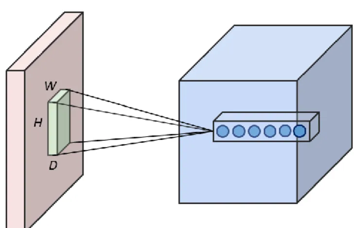
Different from typical artificial neural networks, CNNs exploit the spatially local correlation presented in natural images and have three distinguished features: 3D volumes of neurons, local connectivity, and shared weights. A CNN arranges neurons in a layer in three dimensions (Figure 2-4): width, height, and depth. Here depth means the third dimension of a feature map volume, while the depth of a Neural Network refers to the total number of layers in a network. The neurons in a layer are only connected to a small region of the layer precedes to it. Besides, CNNs exploit spatial locality by enforcing a local connectivity pattern between neurons of adjacent layers. Also, each convolutional kernel is applied across the same image. That is, the same convolutional kernel is applied at many locations in the image and the same weight is shared.

(24)

A typical CNN contains convolutional, pooling, and fully connected layers.

Different types of layers are connected locally and stacked together to form a CNN architecture. In CNNs, a convolutional layer convolves with input feature maps and generate output feature maps. A filter in a convolutional layer has size W × H × D, where W is the width of the filter, H is the height of the filter, and D is the number of input feature maps. For each input feature map, each W × H values of the W × H × D weights are used as a convolutional kernel for one particular input feature map. If we have N filters, each filter will produce an output feature map by convolving with the input feature maps. For example, in Figure 2-5, a W × H × 3 filter convolves with three input feature maps of size 32 × 32 and produces an output feature map of size 30 × 30.

Figure 2-5: A filter is used to produce a new feature map.

Instead of predefining by humans as common convolution kernels, CNNs learn the values of convolution kernels during the training process. To reduce the computational complexity of 2D convolution, a convolutional layer only connects each neuron in a feature map with a small region of the input. In Figure 2-6, multiple neurons at the same

(25)

location in the output feature maps are connected to the same region in the input feature map. This spatial connectivity is controlled by a filter size, for instance, the filter of size W × H × D defines the spatial connectivity between the input and output feature maps.

During the forward pass, each convolutional kernel convolves with any possible position in an input feature map and a new feature map will be generated.

Figure 2-6: Local connectivity of a convolutional layer.

Pooling layers perform similar operations as convolutional layers, but the operations of pooling layers find the maximum (max pooling) or the average value (average pooling) within the region defined by a 2D window (Figure 2-7 assumes a 2 × 2 window with stride 2 for pooling and each color represents the pooling position and the result.) It is common to periodically insert a pooling layer in-between convolutional layers in CNNs. The purpose of a pooling layer is decreasing the spatial size of a feature map and the number of parameters. In addition, computation in the network will also be reduced. Also, pooling layers are not involved in the training process of CNNs and have no parameters associated with them since the operations of them are fixed and

(26)

Figure 2-7: Illustration of the max pooling operation.

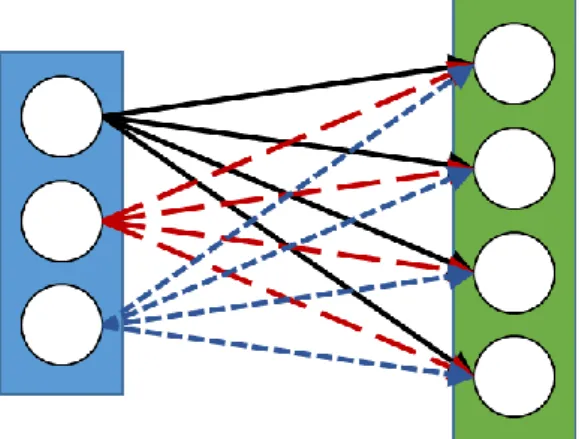
Finally, a fully connected layer is a layer that has full connections to the previous layer, i.e., each neuron in a fully connected layer has connections to all neurons in the previous layer. Figure 2-8 illustrates the idea of full connections. In Figure 2-8, the green one on the right is a fully connected layer that each neuron (the white circle) connects to all neurons in the previous layer (the blue one) and connections to these neurons are represented by lines with different colors. As a result, a fully connected layer has dense connections between neurons and a significant amount of storage and computation is required.

Figure 2-8: Illustration of a fully connected layer.

(27)

In addition to aforementioned layers, non-linear activations and normalization layers can also be found in a CNN. The non-linear activation is used to apply a non-linear transformation to the output of a convolutional or a fully connected layer.

Common non-linear functions used in CNNs are rectified linear unit (ReLU), sigmoid, and hyperbolic tangent (tanh). Figure 2-9 shows function plots for these non-linear functions. ReLU is defined as follows:

The sigmoid function is defined as

Figure 2-9: Plots for various non-linear activation functions.

(Left: ReLU, center: sigmoid, right: tanh)

A normalization layer is usually used to improve training efficiency and model accuracy by controlling the input distribution across layers. Batch normalization [28] is a common practice used in normalization layers, which performs the normalization for each training mini-batch. Usually, the distribution of the layer input is normalized to a zero mean and a unit standard deviation. In batch normalization, the normalized input value is scaled and shifted.

(28)

A common pattern of CNN architecture is stacking together a convolutional layer, a ReLU activation layer, and a pooling layer. The pattern repeats until the image has been downsampled to a small size. Finally, fully connected layers are appended to the end of CNN and the last fully-connected layer holds the output, such as the class scores.

Many deep CNNs have been proposed over the past two decades, and each proposed CNN has a different network architecture concerning the arrangement of layers, for example, type of layers, the order of layers, and the number of layers to be used. In addition, the configuration of filters separates one CNN from the other. The configuration of filters can be the width and height of the filter or the depth of the filter.

Figure 2-10: Architecture of VGG-16.

VGG-16 proposed by Simonyan et al. [29] is a widely adapted CNN architecture (Figure 2-10). It consists of 16 layers: 13 convolutional layers and 3 fully connected layers. The core idea of VGG-16 is using smaller filters (3 × 3) that have fewer weights

(29)

to achieve the same effect as larger 5 × 5 filters. Therefore, all convolutional layers in VGG-16 have the 3 × 3 filter size. In addition, the three fully connected layers at the end of the network have 4096, 4096, and 1000 neurons, respectively.

2.5 Semantic Segmentation

In semantic segmentation, the goal is labeling every pixel in an image with a semantic meaning. A label usually describes a specific class of objects, in an urban road scene, for example, pixels are labeled as the sky, car, or pedestrian. The problem of semantic segmentation is dense prediction comparing to other vision problems, such as image classification and object detection. Generally, there are three categories of computer vision problems and each has different level of complexity (see Figure 2-11).

The task of semantic segmentation needs to predict a label for every pixel in an image while image classification or object detection only need to make predictions for the whole image or parts of the region within an image.

(a) Image classification (b) Object detection (c) Semantic segmentation Figure 2-11: Comparison of different vision problems. [30]

Before deep CNNs have been widely used in solving vision tasks, most methods relied on handcrafted features to predict pixels independently. In this kind of approaches, an image patch is usually fed into a classifier such as Random Forest or Boosting to

(30)

object classification has attracted researchers to take advantage of their feature learning capabilities for semantic segmentation. Most state-of-the-art deep CNN architectures [5, 31] designed for segmentation learn to encode an input image into a low resolution image representations and decode them to the original resolution with pixel-wise prediction.

For evaluating the performance of a semantic segmentation system, three metrics are commonly used: per-pixel accuracy, per-class accuracy (class average accuracy) and average precision [32]. Per-pixel accuracy is defined by the percentage of correctly classified pixels in the test set:

where Ncorrect is the number of correctly classified pixels in an image and N is the total number of pixels in the image.

As for per-class accuracy, it is defined as follows:

where C is the total number of classes in the dataset, N^’i is the total number of correctly classified pixels of class i ∈ {1, 2, … C}, and Ni is the total number of pixels of class i.

The average precision (AP) for a class is defined as the intersection over union metric.

For a given object class c, we compute a ratio between the intersection and the union of two sets, that is, the ground truth pixels and the predicted pixels for class c.

In addition, mean average precision (mAP) is commonly used to evaluate over all classes in the dataset:

(31)

where C is the total number of classes in the dataset and i is an object class that i ∈ {1, 2, …, C}.

Since the success of CNNs for object classification, researchers have taken advantage of its learning capabilities to tackle problems of semantic segmentation.

Recent CNNs for semantic segmentation usually exploit the encoder-decoder architecture [5, 31, 33]. Fully Convolutional Network (FCN) proposed by Long et al. [5]

is the forerunner of this kind of architecture. In an encoder-decoder CNN architecture, the network architecture is divided into two parts. The first part is the encoder network that encodes input images into lower resolution spatial features. VGG-16 [29] is commonly adapted for the encoder network. Then, another part called decoder network will learn to upsample these low resolution feature maps to original input resolution and predict class labels for each pixel. The decoder network learns to upsample feature maps for the next decoder in the hierarchy by combining output feature maps from multiple encoders in the encoder network. For example, a deconvolutional layer will be applied to fuse and upsample the feature maps to a segmentation score map.

Most recent deep CNN approaches for semantic segmentation have a similar architecture of encoder network and they are mainly different in the design of decoder network and the way of training. Some researches exploit multi-scale CNNs to deal with semantic segmentation [34, 35]. The core idea of this approach is using features extracted at different scales to obtain local and global contexts. Feature maps from early encoders can provide sharper object boundaries because of higher frequency details

(32)

within them. However, the test time of this approach is expensive since feature extractions are performed in multiple paths of CNNs.

(33)

Chapter 3 Methodology

3.1 System Overview

We design a vision-based autonomous driving system that maps visual sensory inputs to driving controls. In this thesis, we only consider visual sensory input from a front-facing camera and the autonomous driving system learns how to steer through imitation learning. To collect data, human drivers collects images and corresponding steering angles as a reference policy.

The overall system is illustrated in Figure 3-1, and the system design is based on the knowledge in Section 2.1. Because of the learning capacities of deep CNNs, we can utilize it to compute semantic segmentation from a raw RGB image. Also, deep CNNs can also be used to map high level visual representation such as semantic segmentation to driving controls such as steering. Therefore, we can construct a vision-based autonomous driving system that uses deep CNNs to solve visual perception and steering control problems. In our proposed system, a deep CNN is used as the cognition module, while another deep CNN functions as the decision making module and the control module. The Perception Network is used to generate semantic segmentation and the Control Network generates steering values based on the result of the perception module.

(34)

The proposed method is based on intermediate semantic perception. Instead of simply taking an end-to-end CNN approach [9] with raw RGB images as inputs, we first process the input image to get an understanding of the road scene. We generate a high level understanding of the scene and use it as an extra supervision to train a steering prediction model. In general, two steps are involved in the proposed approach. First, we use a deep CNN to generate semantic segmentation from an image as an intermediate perception. Then, the segmentation result is used to feed another deep CNN to predict steering. The first step is used to parse the whole image so that a high level information of the scene is obtained. The semantic segmentation obtained from this step describes the scene layout, for example, which part of the input image represents sky or road.

After obtaining a semantic scene layout, we use this information to facilitate learning of car steering since the segmented result provides semantic information which reveals the specific part of the image we should focus on and the part of the image that can be ignored.

3.2 Semantic Segmentation Generation

As mentioned above, the first stage is semantic segmentation generation. In this stage, we use SegNet [36] as the CNN infrastructure for the Perception Network.

SegNet is designed to be efficient enough for solving pixel-wise semantic segmentation.

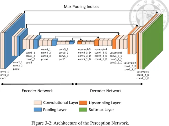
It is efficient for road scene understanding both in memory and computation. In addition, SegNet can delineate small objects in a scene properly. Besides, training of SegNet can be performed end-to-end. The architecture of SegNet is an encoder-decoder approach (Figure 3-2) that is inspired by the unsupervised feature learning architecture proposed by Ranzato et al. [37].

(35)

Figure 3-2: Architecture of the Perception Network.

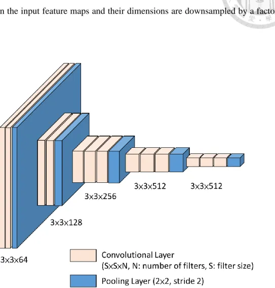
3.2.1 Encoder Network

The first part of the network is an encoder network that produces low resolution feature maps. In SegNet, the encoder network has 13 convolutional layers that correspond to the first 13 convolutional layers in VGG-16 (Figure 3-3). However, the encoder network and decoder networks do not have any fully connected layers. The absence of fully connected layers makes parameters of the encoder fewer and easier to train than other CNN architectures for semantic segmentation [5, 31]. Each encoder block in the encoder network is composed of some convolutional layer with ReLU non-linear activation (from 2 to 3) and each convolutional layer is followed by a batch normalization layer. A max-pooling layer is attached to the end of an encoder block. The convolutional layer of an encoder block convolves with input feature maps to produce

(36)

the output feature maps. Following that, ReLU non-linear activation is applied. At the end of an encoder block, a max-pooling layer with a 2 × 2 window and stride 2 is applied on the input feature maps and their dimensions are downsampled by a factor of 2.

Figure 3-3: Architecture of the encoder network.

The effect of max-pooling is used to achieve translation invariance over small spatial shifts in an input feature map and the sub-sampling brings in a large spatial context from an input feature map for each pixel in the output feature map. A sequence of encoders can achieve more translation invariance for better classification results;

however, there is a loss of spatial resolution of the feature maps. This increasingly loss of spatial resolution of the feature maps can affect the results of segmentation since boundary details between objects also get lost. Therefore, feature map information

(37)

before downsampling should be stored for later uses. To keep this information, we store the input feature maps of a max-pooling layer. To save memory usage, max-pooling indices can be used. Note that max-pooling indices are the locations of the maximum feature value in a 2 × 2 pooling window during max-pooling and they are stored for each input feature map to the max-pooling layer. The storage required for max-pooling indices of a feature map is 2 bits for each 2 × 2 pooling window (Figure 3-4) since we only need to remember the maximum location among all 4 locations within the window.

Figure 3-4: Illustration of max-pooling indices.

In Figure 3-4, each color means the correspondence between blocks. Besides, the possible value of max-pooling index can be {0, 1, 2, 3}, where 0 is the top-left location, 1 is the top-right location, 3 is the bottom-left location, etc. In this way, it is more efficient to store than storing a full size feature map although the accuracy will decrease slightly.

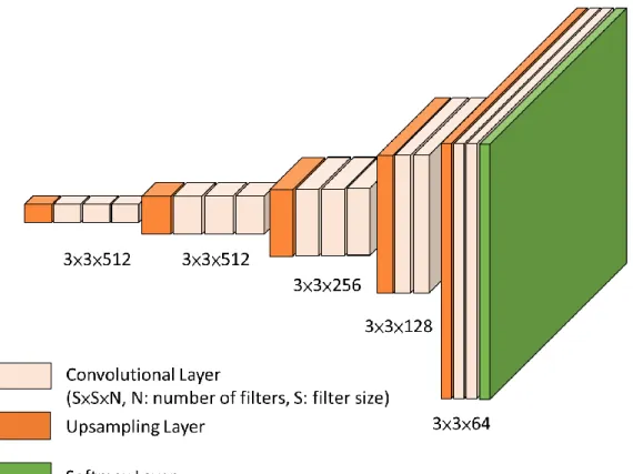
3.2.2 Decoder Network

The second part of the network is a decoder network which is responsible for producing multi-dimensional features for each pixel for classification. The architecture

(38)

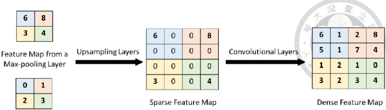
sequence of decoder blocks and each block consists of an upsampling layer in the beginning and some convolutional layers (from 2 to 3) with ReLU activation. Besides, similar to the encoder network, a batch normalization step is applied to the output feature maps from each convolutional layer. Each decoder block has a corresponding encoder block. Therefore, the decoder network also has 13 convolutional layers, and the decoder blocks are arranged in a hierarchical order such that the blocks with smaller input dimension are in the front. Each decoder block performs non-linear upsampling of input feature maps by the max-pooling indices received from the corresponding encoder block. The resulting upsampled feature maps are sparse, and therefore, series of convolutional layers are used to produce dense feature maps. The decoding process of SegNet is illustrated in Figure 3-6.

Figure 3-5: Architecture of the decoder network.

(39)

Figure 3-6: Illustration of the decoding process.

After a series of decoding steps, high dimensional features maps that have the same resolution as the input to the encoder network will be obtained from the final layer of the decoder network. The high dimensional features maps are fed to a softmax classification layer which classifies each pixel independently. The output of the softmax classifier is a C-channel image of object class probabilities where C is the number of classes. The result of semantic class assignment for each pixel is obtained by finding the class with the maximum class probability. Finally, the whole network is trained with per-pixel cross entropy loss:

where N is the number of samples, W and H are width and height of the input image, Y(x, y) is the class label for the pixel location (x, y) in the ground truth mask Y, and P(x, y)

is the predicted class label for the pixel location (x, y) in the network output P.

(40)

3.3 Car Steering Angle Prediction

After obtaining semantic segmentation from the previous stage, we are moving into the second stage. The result of the semantic segmentation is a 2D map that marks each pixel in the original input with a label, which is an integer value that represents a class. For example, a value of 2 represents the road class, and pixels in the input image are labeled with 2 if they are covered by roads. Also, since the input to the second stage is a 2D segmentation map, we utilize a CNN based approach to extract features from the map and predicting steering angles. In this stage, we use a CNN called the Control Network to predict steering angles from the segmentation result.

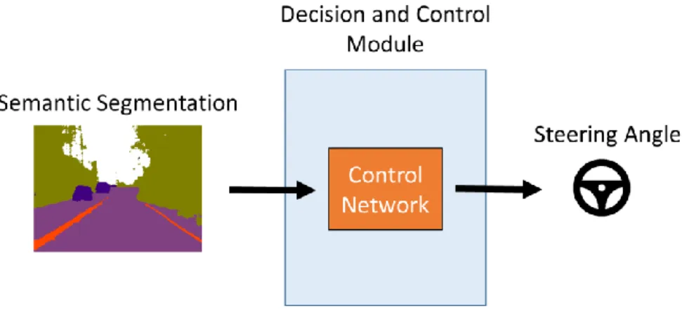
Figure 3-7: Overview of the second stage.

Figure 3-7 provides a high-level overview of the second stage. In our system, the Control Network serves as decision and control modules in an autonomous driving system because the system only solves the lane following problem and does not deal with other high-level decision problems, such as switching lanes or overtaking previous cars. The Control Network decides how to drive along the lane based on the input semantic segmentation and executes the decision by adjusting steering angles.

(41)

Since the segmentation result has removed many details from the input image, the design goal of the Control Network is compactness and efficiency. A compact CNN architecture is preferred since the segmentation map contains few features. Besides, we want to reduce the computation time and achieve promising results at the same time.

Therefore, the Control Network should have as fewer layers as possible and does not contain any complex structures.

The basic idea of the Control Network is to downsample the segmentation map and feed it to a fully connected layer for steering angle prediction. The Control Network architecture for mapping a semantic segmentation to a steering angle is shown in Figure 3-8.

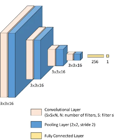
Figure 3-8: Architecture of the Control Network.

(42)

The Control Network is composed of 4 blocks and each block has a convolutional layer with 16 filters of size 3 × 3 and a 2 × 2 max-pooling layer with stride 2. Following each convolutional layer, a max-pooling layer is appended to downsample the output feature maps of each block. Finally, two fully connected layers with 256 and 1 neuron, respectively, are attached to the end of the Control Network. The last fully connected layer will predict a steering angle value.

To meet our design goal, the 3 × 3 filter size is used in a convolutional layer. When using a small filter size such as 3 × 3 in a convolutional layer, finer and local information may be preserved during feature extraction. On the other hand, using larger filter sizes, such as 5 × 5 and 7 × 7 in a convolutional layer, more context will be considered, but finer and local information may be lost. Also, using smaller filter size can result in faster execution and smaller model size.

Another design choice of the Control Network is the number neurons in a fully connected layer. Basically, the number of neurons in a fully connected layer affects the execution time and model size. More neurons in a fully connected layer result in longer execution time and larger model size. In addition, the number of neurons decides the learning capacity of the network. When the number of neurons is large, the CNN has a better learning capability, but it also has more chances to overfit the training data.

Therefore, the final number of neurons of the second to last fully connected layer is 256, which is the optimal value found by experimenting different values.

In general, the parameters of the Control Network is driven by empirical results.

For example, we have conducted an experiment to change the number of convolutional

(43)

of a convolutional layer and a max-pooling layer bring the best outcome. Besides, from the experiment, using 16 filters of size 3 × 3 proves to have the best result. In addition, we have conducted experiments to replace each max-pooling layer with a convolutional layer of 16 3 × 3 and stride 2 filters. Both of these configurations can downsample a feature map by a factor of two, but using a max-pooling layer has a better result.

The output representation is an important design decision in the network architecture. In an autonomous driving system, the Control Module outputs a driving control, e.g., a steering angle. In general, the output driving controls should be continuous scalar values. Therefore, the output of the Control Network should represent a steering angle value that reflects the input semantic segmentation. Also, the output steering angles should be continuous and range from sharp left to sharp right. Therefore, we consider a single value representation for the output of the Control Network.

The single value representation uses a one-neuron fully connected layer to represent a steering angle value, which is shown in Figure 3-8. The goal of the Control Network is predicting a steering angle from a segmentation map which can be viewed as a single value regression problem. Therefore, in order to solve steering angle prediction, mean square error (MSE) is used as the loss function for training the Control Network.

MSE is defined as the following equation:

where ŷi is the prediction for i-th training sample, yi is the actual value for the i-th training sample, and N is the number of total training samples.

(44)

Chapter 4 Experiments

In the experiments, we use Udacity Self-Driving Car Challenge 2 Dataset [38] as a benchmark for the proposed approach. The challenge requires a model to predict steering angles from input images. We have conducted various experiments and show that the proposed method is more robust than the typical end-to-end CNN approach with an RGB image as input.

4.1 Environments

The hardware and system environments are summarized in Table 4-1. Basically, our experiments ran on an Ubuntu PC with Intel i7 3.5GHz CPU, 16GB of memory, and a NVIDIA GTX 1070 GPU.

CPU Intel Core i7-2700K 3.50GHz

(Quad-Core)

Main Memory 16GB

GPU NVidia GeForce GTX 1070

(with 8GB memory)

Operating System Ubuntu 14.04 LTS 64-bit

Table 4-1: Hardware specification for the experiment.

(45)

4.2 Dataset

4.2.1 Cityscapes Dataset

The Cityscapes Dataset [39] provides large data for pixel-level and instance level semantic labeling and focuses on real world urban scenes. Data in the dataset is collected across 50 cities in Europe and captured in different seasons. The dataset contains 5,000 images with fine annotations and each image in the dataset has a resolution of 2048 × 1024 pixels. Examples images and their annotations from the dataset are shown in Figure 4-1. The dataset defines 30 different labels and only 19 of them are used for training and evaluation. In our work, we use pre-trained weights on the Cityscapes dataset and fine-tune the Perception Network.

4.2.2 Udacity Self-Driving Car Challenge 2 Dataset

The Udacity Self-Driving Car Challenge 2 Dataset consists of 33,808 images for the training set and 5,614 images for the test set. Each image in the dataset is in RGB format and has a size of 640 × 480 pixels. Figure 4-2 shows several example images from the dataset. The dataset contains challenging driving scene in different lighting, road, and traffic conditions, for example, shadows, uphill, and heavy traffic. All these images are captured from a front-facing camera installed on a car and we ignore images captured from others cameras (the left and right cameras). In addition, the data were collected by humans driving on urban roads during the daytime. The dataset also includes car motion history such as speeds and steering angles, but we only use steering angles as the ground truth label. The recorded steering angles capture human performance and the value ranges from -2.0 to 2.0 (sharp right to sharp left).

(46)

Figure 4-1: Example images and annotations from the Cityscapes dataset.

(47)

Figure 4-2: Example images from the Udacity Self-Driving Car Dataset.

(48)

4.3 Evaluation Metrics

The evaluation metrics used in the experiments are absolute error (AE), mean absolute error (MAE), and root mean squared error (RMSE). AE is used to measure the absolute difference between the predicted value and the actual value. In addition, it is used to evaluate the performance of a single prediction. The absolute error (AE) is defined as:

where ŷi is the prediction for i-th sample, yi is the actual value for the i-th sample.

Each CNN model will be evaluated by RMSE and MAE. RMSE and MAE are common measurements for evaluating the accuracy of a regression model. The definition of RMSE is defined as:

where ŷi is the prediction for i-th sample, yi is the actual value for the i-th sample, and N is the number of samples. And MAE is defined as the mean of AE over some samples.

4.4 Implementation Details

4.4.1 Semantic Segmentation Annotation for Udacity Dataset

Because the Udacity dataset does not have semantic segmentation annotations, we have to construct ground truth annotations for images in the dataset. First of all, we define 7 classes: Sky, Road Marking, Road, Construction, Car, Vegetation, and Background. The Construction class represents various structures that separates two

(49)

areas and those locating on the side of the road to prevent accidents, for example, fences and guard rails; the Vegetation class includes vertically and horizontally growing vegetation, for instance, trees and grasses; finally, the Background class includes other objects not immediately related to car steering, for example, buildings, traffic signs, etc.

Generally, images from the Udacity dataset are frames from videos recorded during driving. Since consecutive frames in videos are similar, we take advantage of this fact to prevent labeling every image in the dataset. The videos in the dataset were recorded at 20 FPS, so we labeled images every 120 images (frames) on average and totally 335 images are labeled. To generate ground truth annotations for the remaining images, we first fine-tuned a pre-trained SegNet model with these 335 manually labeled images.

Finally, we used the fine-tuned model to generate pixel-wise labels for all images in the Udacity dataset.

4.4.2 Baseline Model

The baseline model serves as a reference for the performance of a typical end-to-end CNN with a raw RGB image as input. We modify a VGG-16 network to have two fully connected layers with 256 neurons and 1 neuron, respectively. In addition, we downsample images from Udacity dataset by a factor of 2 to have an image size of 320 × 240 pixels. The reduced size of the input image enables us to use a larger batch size for efficient training. Finally, the network is trained with Adam optimizer [40]

using a learning rate of 1 × 10^-4with a batch size of 32.

4.4.3 Perception Network

The Perception Network is based on SegNet and it is pre-trained with Cityscapes

(50)

annotations for Udacity dataset. Images from Udacity dataset are downsampled to 320 × 240 pixels for efficient training. Also, the network is trained with Stochastic gradient descent [41] with a batch size of 32. The initial learning rate is set to 1 × 10^-3. Besides, weight decay and momentum are set to 5 × 10^-4 and 9 × 10^-1, respectively. Finally, we fine-tuned the network for 800 iterations with a batch size of 8.

4.4.4 Control Network

The Control Network is trained with semantic segmentation results of images in the Udacity dataset and the corresponding steering ground truths. Semantic segmentation results are downsampled to 320 × 240 pixels for efficient training. In addition, the network is trained with Adam optimizer [28] using a learning rate of 1 × 10^-6 with a batch size of 32.

4.5 Results

4.5.1 Overall Performance

The overall result of the proposed model is promising. We compare the performance of the proposed model and the baseline model in Table 4-2 (the definition of the baseline model can be found Section 4.4.2). The proposed approach outperforms the baseline model in several aspects. First of all, the proposed model is more robust than the baseline model concerning RMSE. The proposed model has an RMSE of 8.85

× 10^-2 on the test set while the baseline model has an RMSE of 9.2 × 10^-2. The mean absolute error of the proposed model is slightly higher than the baseline; however, it has more stable results than the baseline approach since it has a lower standard deviation of the absolute error.

(51)

Model RMSE Mean Absolute Error (± Std. Deviation)

Training Time (Epochs)

Baseline 0.0920 0.059±0.071 47

Ours 0.0885 0.065±0.060 35

Table 4-2: Result on the test set of Udacity dataset.

Team Name Rank RMSE Approach

komanda 1 0.0512 3D CNN [42] and RNN [43]

rambo 2 0.0559

Using two consecutive images as input [43]

chauffeur 3 0.0572 CNN and RNN [43]

lookma 4 0.0716 N/A

5 0.0743 Use ResNet50 [44, 45]

epoch 6 0.0789

CNN with data augmentation and output smoothing [46]

Proposed Model N/A 0.0885 CNN with semantic perception

Baseline Model N/A 0.1121 CNN

bitas 7 0.0944 N/A

ai-world 8 0.0988 N/A

bauer 9 0.1057 N/A

fsc3 10 0.1202 N/A

Table 4-3: Results on the Udacity Self-Driving Car Challenge 2 leaderboard.

(52)

In addition, Table 4-3 shows the results of the baseline model and our proposed model on the Udacity Self-Driving Car Challenge 2 leaderboard [47]. Most of the top teams do not simply use a CNN model, for example, some of them using both CNN and RNN (Recurrent Neural Network) [48]. Besides, some of them take advantage of temporal information and use consecutive images as inputs. On the other hand, our proposed model is based on CNNs and only use a single image as input. If our result would be submitted to the challenge, we would rank 7. However, most of the top results come from more complex techniques and computation. Among those teams using only CNNs our model would rank second (third if team lookma uses CNNs).

Figure 4-3: Absolute errors of the baseline model across the test data.

(53)

Figure 4-4: Absolute errors of the proposed model across the test data.

Also, the overall prediction error from the proposed model is more stable. We compared prediction errors from both models and found that the baseline model has large errors in many test cases. On the other hand, our proposed model is more stable and has smaller errors. For example, in Figure 4-3, there are many test cases that have absolute errors more than 0.4, while in Figure 4-4 the proposed approach has relatively few such cases.

4.5.2 Analysis of Error Cases

To compare the performance between the baseline and the proposed model, we analyze selected error cases for the baseline model. Here, we define an error case as a sequence of frames in the test set that the baseline model predicts with an error over a threshold. An error case reflects the weakness of the baseline model. Based on the information in Figure 4-3, we define an error threshold 0.3 and select three error cases

(54)

of the baseline model for further analysis. Table 4-4 gives a summary of the mean absolute errors (MAEs) for all error cases.

Model

Mean Absolute Error (± Std. Deviation)

Error Case #1 Error Case #2 Error Case #3

Baseline 0.516±0.079 0.438±0.088 0.344±0.019 Ours 0.183±0.111 0.198±0.124 0.091±0.054

Table 4-4: Mean absolute errors and standard deviations for all error cases.

In addition to MAE, in the following analysis, we will investigate the average feature map that obtained from the layer just before the fully connected layer.

Specifically, we investigate the average feature maps that obtained from the 4th max-pooling layer of the proposed model and the 5thmax-pooling layer of the baseline model. The averaged feature map is generated by summing and averaging values of each pixel from all output feature maps of the last max-pooling layer.

Figure 4-5 shows an image (frame 1857) from the first error case of the baseline model. In this case, the baseline model has the worst performance and has an MAE around 0.516. On the other hand, our proposed model can handle this test case with an MAE around 0.183. An overview of the performance comparison between both models can be found in Figure 4-6, which shows the prediction results of both models. Also, from Figure 4-6, we can see that the proposed model has more accurate prediction than the baseline model. This test case represents a scenario that a lot of background objects appear in the image and the baseline model fails to extract important features from the

(55)

training data to help the CNN recognize the centerline marking and relate it to the steering angle. However, the proposed model uses semantic segmentation and is able to recognize regions that are important for driving, e.g., the road and the centerline marking. Besides, the proposed model can map these important features to steering angles. The segmentation result in Figure 4-8 shows that the road region and centerline marking are identified (see Figure 4-9 for color mapping). The average feature maps of both models also show that the proposed model is able to extract and highlight important features, such as the road and the centerline marking, while the baseline model cannot (Figure 4-7).

An image from the second error case of the baseline model is shown in Figure 4-10.

Overall, the proposed model has a better accuracy than the baseline model, which is reflected in Figure 4-11. In this error case, the baseline model has an MAE around 0.438.

On the other hand, our propose model can handle this error case with an MAE around 0.198. This error case also shows that the proposed model cannot recognize important region such as the centerline marking. From Figure 4-12 and Figure 4-13, it shows that the proposed model is able to extract features of centerline markings, while the baseline model cannot.

In Figure 4-14, an image from the third error case of the baseline model is shown.

In this error case, the baseline model has an MAE around 0.344. On the other hand, our proposed model can handle these test case with an MAE around 0.091. From Figure 4-15, we can see that the proposed model outperforms the baseline model with much higher prediction accuracy.

(56)

Figure 4-5: An image from error case #1 (frame 1857).

Figure 4-6: Prediction results of error case #1.

(57)

Figure 4-7: Comparison between feature maps from different models (frame 1857).

(a) Baseline model

(b) Proposed model

(58)

Figure 4-8: Result of semantic segmentation for frame 1857.

Figure 4-9: Semantic meaning and the corresponding color

This test case represents a driving scenario that lacks lighting. An RGB image with low lighting may cause the CNN fail to extract important features from the image, e.g., lane markings and side of the roads. However, the proposed model can handle such case and recognize roads and lane markings (segmentation result can be found in Figure 4-16). In Figure 4-17 (a) we can see that the baseline model does not extract any important features, while in Figure 4-17 (b), it shows that proposed model can successfully extract road edges as features.