Journal of Photogrammetrty and Remote Sensing

第 二 十 一 卷 第 四 期 中華民國一○五年十二月

ISSN 1021-8661 DOI: 10.6574/JPRS

Journal of Photogrammetrty and Remote Sensing

Volume 21 No.4 December 2016

Published by Chinese Society of Photogrammetrt and Remote Sensing

航 測 及 遙 測 學 刊

Journal of Photogrammetry and Remote Sensing

發行人：史天元

出版者：中華民國航空測量及遙感探測學會 地址：台北市文山區羅斯福路五段 113 號三樓 信箱：台北市郵政 93-158 號信箱

電話：886-2-8663-3468 886-2-8663-3469 傳真：886-2-2931-7225

電子信件：[email protected] 網址：http://www.csprs.org.tw

PUBLISHER:Peter Tian-Yuan Shih

PUBLISHED BY: Chinese Society of Photogrammetry and Remote Sensing

Address: 3F, No.113, Sec.5, Roosevelt Road, Taipei, Taiwan Mail Address: P. O. Box. 93-158, Taipei, Taiwan

Tel: 886-2-8663-3468 886-2-8663-3469 Fax: 886-2-2931-7225

E-mail：[email protected] Web Site：http://www.csprs.org.tw 總編輯

曾義星

國立成功大學測量及空間資訊學系 電 話：886-6-275-7575 分機 63835 傳 真：886-6-237-5764

電子信件：[email protected]

EDITOR-IN-CHIEF Yi-Hsing Tseng

Department of Geomatics, National Cheng Kung University Tel: 886-6-275-7575 ext. 63835

Fax: 886-6-237-5764

E-Mail: [email protected] 編輯委員(依中文姓氏筆劃排列) EDITORIAL BOARD

王素芬 (彰化師大) 王聖鐸 (師範大學) 江凱偉 (成功大學)

S. F. Wang (National Changhua University of Education) S. Wang (National Taiwan Normal University)

K. W. Chiang (National Cheng Kung University) 何宗儒 (海洋大學) C. R. Ho (National Taiwan Ocean University) 林昭宏 (成功大學) C. H. Lin (National Cheng Kung University) 邱式鴻 (政治大學) S. H. Chio (National Chengchi University) 林老生 (政治大學) L. S. Lin (National Chengchi University) 林唐煌 (中央大學) T. H. Lin (National Central University) 周天穎 (逢甲大學) T. Y. Chou (Feng Chia University)

洪榮宏 (成功大學) J. H. Hong (National Cheng Kung University) 徐百輝 (臺灣大學)

陳朝圳 (屏東科大)

P. H. Hsu (National Taiwan University)

C. T. Chen (National Pingtung University of Science and Technology) 張中白 (中央大學) C. P. Chang (National Central University)

黃金聰 (臺北大學) J. T. Hwang (National Taipei University) 曾義星 (成功大學) Y. H. Tseng (National Cheng Kung University) 詹進發 (政治大學) J. F. Jan (National Chengchi University) 楊明德 (中興大學) M. D. Yang (National Chung Hsing University) 蔡富安 (中央大學) F. Tsai (National Central University)

蔡榮得 (中興大學) J. D. Tsai (National Chung Hsing University)

封面照片說明 About the Cover

時空資訊的紀錄，能幫助我們了解時代變遷之現象。封面照運用了日治時期的古地圖、早期歷史 航照、經建版地形圖、以及現代影像，呈現了台南古都沿海地區之水域變遷、產業變遷、聚落變遷，

藉由百年時空地理資訊的建立可以讓過去歷史事件更真實且更清晰地被描繪出來，顯示了多時期的時 空地理資訊有助於過去的變遷研究。

航測及遙測學刊 第二十一卷 第 4 期 第 213-226 頁 民國 105 年 12 月 213 Journal of Photogrammetry and Remote Sensing

Volume 21, No.4, 2016, pp. 213-226 DOI：10.6574/JPRS.2016.21(4).1

1國立成功大學測量及空間資訊學系 碩士 收到日期：民國 104 年 05 月 25 日

2國立成功大學測量及空間資訊學系 教授 修改日期：民國 105 年 08 月 26 日

*通訊作者, E-mail: [email protected] 接受日期：民國 105 年 10 月 13 日

以時空資訊探討百年來台南古都沿海地區的 土地利用變遷

江若慈

^1*

曾義星

²

摘要

時空資訊的紀錄，能幫助我們了解時代變遷之地理現象，自 20 世紀以來，台灣開始出現經過精細測 量之圖資，包括地形圖及航照影像，然而欲應用時空資訊，必須將其糾正對位到一致的坐標系統上。本 研究利用航測軟體(SOCET GXP 4.0)以及六參數轉換進行糾正對位，使用(1)古地圖：1904 年台灣堡圖及 1921 年台灣地形圖(2)1947-1948 年及 1970 年代歷史航照影像(3)1985-1989 年第一版經建版地形圖(4)2009 年福衛二號衛星影像(5)2010 年正射影像，建立了百年圖資對位處理流程，及對其精度進行評估，其中古 地圖及美軍空軍航照之精度大約可達十餘公尺，而 1970 年代歷史航照經過空三之正射影像精度可達約 2 公尺，並以台南古都沿海地區(約今安平一帶)為研究範圍，探討其土地利用的變遷，藉由影像判釋數化九 項土地利用類別來量化土地利用變遷資料，以及透過轉移矩陣了解各土地利用如何轉變，並且配合文史 資料探討及呈現其土地利用變遷的過程。

關鍵字：土地利用變遷、時空資訊、沿海地區、安平

1. 前言

1.1 研究動機與目的

台南是台灣最早發展的城市，在將近四百年 前，台南沿海形成一座潟湖，稱為台江內海，當 時大型船隻可在此航行與停靠，曾經扮演台灣重 要的貿易門戶；而今台江內海已漸漸陸化，其地 理環境產生如此巨大變化，進而影響了土地利用 的轉變。安平則位於台江內海的南端，因此在歷 史定位上扮演重要的角色；然而，在早期台灣的 歷史文獻大多僅著墨於文字上的敘述，我們能了 解過去某段時間所發生的歷史事件，卻缺乏歷史 文獻中所述史事之地理空間的相互對照，閱讀者 往往只能想像歷史事件的空間關係，廖怡雯(2003) 在歷史脈絡的變遷分析中曾談到以文字描述來

探討歷年來土地利用變遷的事實以及情境的方 法主要是從觀察(observe)、描述(describe)及解析 (interpret)來探討，此類方法因其缺乏具體的證據 來說明土地利用變遷的過程及情形，所以無法提 供相關空間特性上的研究成果。為瞭解其空間發 展的轉變，建立時空地理資訊能有助於釐清地理 環境變遷情形，時空資訊為將真實世界的空間資 訊加上時間尺度，成為一個整合的面向 (范毅軍，

2006) ，倘若能將時空資訊與文史紀錄結合對應，

必能成為有利的變遷分析工具。

20 世紀以前的古地圖多屬一種描繪性的地 圖，雖然大多非客觀式的描繪仍然能呈現許多當 時珍貴的資訊，由於古地圖在繪製的當時缺乏精 細的測量基礎與技術，因此大多缺乏正確之坐標 與對位幾何，難以對位至現代之地圖。然而自日 治時期以來，台灣開始出現最早依據西方測繪技

術測繪產出的精細地圖，有 1904 年繪製的台灣 堡圖及 1921 年的台灣地形圖等；二次世界大戰 後期，美軍先後為了軍事偵查及測繪製圖目的拍 攝了台灣最早的航照影像，自 1943 年至 1952 年 間執行許多拍攝任務；在 1954-1976 年間，我國 空軍也以基本地圖測製及國土資源調查為目的，

持續大規模航拍任務；自 1976 年開始為了稻作 調查，也每年進行全面性的航拍，以航照影像判 釋方式取代傳統地面普查，政府也定期繪製多版 基本地形圖；而在現代，藉由衛星影像可快速地 呈現大範圍的地貌資訊。

這些寶貴的空間資料提供我們建立時空地 理資訊的可能性，也成為我們將歷史空間對應到 現今空間的媒介，來補足以往文獻資料的不足。

因此，本研究希望藉由百年的時空資訊來呈現各 時期的土地利用情形，為了進一步描述各時期土 地利用之變遷，同時透過量化各時期各類土地利 用變遷，並透過轉移矩陣之方式來了解各時期土 地利用轉變之情形，做為比較各時期變遷之依據，

以 分 析 台 南 古 都 沿 海 地 區 土 地 利 用 變 遷 的 沿 革。

1.2 相關研究

時空地理資訊可藉由萃取過去歷史圖資的 空間資訊來建立，以呈現過去地表的樣貌，在歷 史圖資中，地圖是歷史環境的文件記錄，在環境 變遷研究上具重要參考價值(賴進貴及葉高華，

2005)，而歷史航照是一項可直接呈現地表樣貌的 重要資訊(Redweik et al., 2010)，因此發展出不少 相關的應用層面，其中以自然環境變遷之應用最 為廣泛。

歷史圖資相關之應用研究如 Cardenal et al.

(2006)以自率光束法進行歷史航照影像對位，並

應用於地滑變遷研究；王超國(2009)利用參數轉 換將台江內海 1904、1928、1985、1999 年等四 個時期的歷史地形圖進行套疊與分析，惟其探討 的時間間隔較大，中間年代之演變過程無藉由歷 史圖資來逐步呈現；莊育侃(2010)運用了歷史航 照與日治時期地形圖資料探討花蓮海岸的地形 變遷，利用數化日治時期歷史地形圖與數位化各 時期航空相片繪製各時期海岸線位置，比較各年 代海岸線的變化關係等，其在歷史地圖之精度約 30 公尺以下的誤差；莊永忠、等 (2011)運用地 理資訊系統(GIS)整合歷史地圖與歷史航照等圖 資，並賦予其地理坐標系統，探討陳有蘭溪集水 區自然環境變遷、人為活動與聚落的發展之空間 關係。

而為了能更進一步了解百年來土地利用之 時空變遷以及充分地運用這些歷史圖資所提供 的訊息，在描述土地利用變遷時轉移機率矩陣度 量為經常使用的計量方法，其可以表現各種類別 的土地利用比例於時間序列上的增減情形，同時 可顯現原先土地利用類別變遷的轉換過程(蔡靜 如，1998)，故本研究藉此方法來探討各時期土地 利用之轉變。

2. 時空資訊

2.1 研究區域

研究區域主要以安平行政區為核心，但變遷 之區域往往難以行政界線劃分研究範圍，因此相 鄰有關聯的地區也一併納入討論，總共涵蓋 32 個里，其北側以鹽水溪及民權路四段為界，東主 要以金華路一至四段為界，南以鯤鯓路為界，西 則以台灣海峽為界，面積約 1,878 公頃，如圖 1 右圖中紅線範圍內。

江若慈、曾義星:以時空資訊探討百年來台南古都沿海地區的土地利用變遷 215

圖 1 研究區域示意圖 (取自 2009 年份福衛二號正射影像)

2.2 日治時期古地圖

日治時期由於統治殖民之需，日本人於 1895 年製作台灣首部經由精細測量的地形圖─臺灣迅 速圖，其比例尺為兩萬分之一，但由於此地形圖 測繪時間較倉促，內容較不精確，因此較廣泛被 使用的地圖為 1904 年完成的臺灣堡圖以及之後 由陸地測量部測繪的地形圖。

臺灣堡圖為日治初期對台灣進行全面丈量 的地圖之一，製作年代從 1900-1904 年，其比例 尺為兩萬分之一，主要針對台灣平原地區進行土 地調查事業，由臨時台灣土地調查局所繪製(林春 吟，2012)，當時丈量是以台中公園為基準，明治 版共有 465 幅圖幅，大正版共有 464 幅圖幅，本 研究使用之臺灣堡圖為明治時期版本。

日治後期基於實施內地延長主義之歷史背 景下，日本人在台繪製多幅基本地形圖，其中比 例尺最大者為 1921-1929 年由陸地測量部所繪製 的兩萬五千分一地形圖(林春吟，2012)，當時平 面測繪是以虎子山為基準，一共有 173 幅圖幅。

2.3 早期歷史航照

台灣最早的航照影像是由美軍所拍攝，目前 現存最早的航照影像是由工研院綠能所典藏，目

前早期歷史航照數化工作已由中央研究院完成 (廖泫銘、等，2011)。

本研究所使用的歷史航照可分為美軍及我 國空軍、以及少部分由農林航測所拍攝之影像，

由於早期航照影像多被視為是機密的資訊，因此 早期由美軍拍攝的影像無法得知其明確的內方 位資訊，此外這些影像重疊情形亦多半不符合標 準航測之規範，因此難以依一般空中三角測量方 法恢復其地理資訊。研究中所使用美軍的航照影 像拍攝於 1947 及 1948 年，一共使用七條航帶共 87 張影像。

1970 年代由我國空軍及農林航測所拍攝的 影像，屬於標準航拍影像，影像符合標準重疊，

因此其內方位資訊可經由相機率定報告得知，並 且在影像上仍存有明確的框標資訊，可依空中三 角測量法恢復其地理資訊。研究中使用的影像大 多於 1975 及 1976 年所拍攝，一共八條航帶共 240 張影像。

2.4 經建版地形圖

內政部自 1985 年起根據台灣五千分之一及 一萬分之一像片基本圖，並經實地調繪製成多版 地形圖，第一至三版地形圖的坐標系統均採用 TWD67，第四版開始坐標系統採用 TWD97，比

例尺為兩萬五千分之一，全台共 263 幅圖，各圖 幅調繪時間不一，其圖幅大小各 7.5'，本研究因 時間序的需求主要使用第一版，第一版成圖時間 在 1985-1989 年間，而本研究範圍圖幅之調繪時 間在 1989 年 (內政部國土測繪中心，2014)。

2.5 現代影像

現代有許多高精度的衛星影像及航拍影像，

本研究使用 2009 年份福衛二號衛星正射影像以 及 2010 年經由航拍產製的正射影像作為現代影 像之依據，並從中選擇影像之控制點與檢核點，

將日治時期古地圖、早期歷史航照等歷史圖資統 一對應至現代影像 TWD97 坐標系統基礎下。

3. 研究方法

3.1 研究流程

時空資訊資料必須建立在統一坐標基準下，

具有相同的基準方能進行比較與應用，為達此目 的，影像的糾正與對位是一項重要的工作，在本 研究中，歷史圖資主要可分為古地圖、早期歷史 航照影像及現代地形圖三類(詳如表 1)。

古地圖由於年代久遠，再加上掃描與圖紙伸 縮變形等誤差，因此，針對古地圖相鄰圖幅銜接 處無法接合者皆先經過相對方位之平移糾正，讓 地圖各圖幅間之特徵能相連，再做絕對方位改正，

於 SOCET GXP 4.0 軟體採用六參數轉換，並以 2009 年福衛二號影像為基準，挑選了過去至今仍

存在的道路交叉點做為絕對坐標轉換的地面控 制點(如圖 2)。

針對歷史航照影像的性質可分為兩大類，其 糾正對位方法依據該航照影像是否有明確的內 方位參數而定，一般而言，我們可以藉由攝影測 量的光束法平差來進行影像方位的糾正，然在早 期航拍影像，其內方位參數並不明確；而外方位 參數由於過去歷史航照拍攝時尚未以 GPS 輔助 空中飛行定位，僅能參考當時的飛航任務航跡圖 (江正雄、等，2006)，而本研究則是藉由一幅參 考影像自行辨認拍攝位置以及計算概略的外方 位資訊。

1970 年代所拍攝的影像符合標準航測影像，

且具有相機參數，因此可遵循一般空中三角測量 的流程進行影像的幾何糾正，並產製出正射影像，

本研究使用商業軟體 SOCET GXP 4.0 產製正射 影像，以 2009 年 2m 解析度的福衛二號衛星影像 作為參考影像，在上面選取現今與過去的不變點 作為控制點進行空中三角測量解算(如圖 3)；而 1947、1948 年份未必符合標準航測規範且不具備 相機參數的影像，因所使用的相機無明確的內方 位資訊，本研究利用數學模式的聯合解算，在無 需相機內方位資訊的情形下，同時求解所有重疊 影像的仿射轉換(Affine transformation)參數，並 以先前產製 1970 年代之正射影像選取相同的特 徵點(如道路交叉口)作為控制點，與航帶內與航 帶間各張影像的連結點，同時平差計算出各張像 片的轉換參數，最後再將各航帶鑲嵌成一幅影像。

圖 2 2009 年福衛影像(左)；1904 年台灣堡圖(右)

江若慈、曾義星:以時空資訊探討百年來台南古都沿海地區的土地利用變遷 217

圖 3 2009 年福衛二號影像(左)；1970 年航照影像(右)

表 1 百年歷史圖資整理

圖資 年份 比例尺/解析

度

幅數 圖幅大小 座標基準 來源

臺灣堡圖 1900-1904 1/20000 465 幅 ( 明 治版)

經度6’ ×緯度 4’ 地 理 坐 標 系

臨時臺灣土地 調查局 日治時期地形

圖

1921-1929 1/25000 173 經度 7.5’ ×緯度 5’

地 理 坐 標 系

陸地測量部

航照影像 1947 年代 約 0.95m 103 約 6.6×6.6km 像坐標系 美軍

航照影像 1970 年代 約 0.3m 240 約 3.6×3.5km 像坐標系 台灣空軍

第一版經建版 地形圖

1989 1/25000 19 經度 7.5’ ×緯度

7.5’

TWD67 國土測繪中心

福衛二號衛星 影像

2009 2m 9 24km TWD97 國家太空中心

本研究使用之現代地形圖為經建版地形圖，

此地形圖成果可靠，因此僅需做坐標轉換處理將 圖資統一轉換至 TWD97 坐標系統，本研究透過 Global Mapper 軟體設定坐標參數進行坐標轉換，

並且將轉換成果鑲嵌為一幅地圖。

將這些圖資整合至 TWD97 坐標系統後，為 了解各歷史圖資之精度，我們利用現代影像選取 檢核點以評估各圖資的誤差，並且將這些圖資建

立於以網路為基礎的多視窗同步瀏覽平台，將成 果發布於網站上作為對位成果之展示，並且利於 影像判讀及變遷之比較。接著透過各年代地圖之 圖例與各年代影像之比較判釋土地利用情形，並 數化各類土地利用，以及計算土地利用變遷轉移 矩陣，最後藉由歷史文獻的輔助分析土地利用變 遷，研究流程如圖 4 所示。

歷史航 照影像

有相機參 數

無相機參 數

正射影 像鑲嵌 利用現代影像 選取地面控制

點

在重疊影像上 選取連結點

空中三角測 量計算

多張影像同 時進行仿射

轉換

鑲嵌影 像 選取地面

控制點 古地圖

糾正相對方位

鑲嵌地 圖

利用現代影像 選取地面控制

點

進行仿射轉 換

現代地 形圖

坐標轉換

鑲嵌地 圖

現代影 像

圖資精度評估

選取檢 核點

建立多視窗平台

影像判釋與數化

土地利用變遷轉移 矩陣

分析土地利用變遷

圖 4 研究流程圖

3.2 影像數化

欲了解土地利用變遷之實際情況，必須透過 各種度量方法以取得土地利用之資訊，以作為後 續分析的基礎(張文菘，2013)。根據 Clawson &

Stewart (1965) 土地利用的定義為人類在土地上 從事所有之活動，而在不同區域的土地利用會反 應當地的自然背景與文化歷史(丁志堅，2002) ， 因 此 各 區 域 之 土 地 利 用 具 有 一 定 程 度 的 獨 特 性。

本研究歷史圖資之數化，以國土測繪中心之 國土利用調查之分類表為基準，針對研究區域內 之土地利用特色而進行調整，以人工數化魚塭、

農作、水域、建成區、鹽田、工業區、沙洲、裸 露地、以及其他共九類，其中其他包含了道路、

林地、墳墓及其他特殊用地，其中此區的林地多

為沿海的防風林，而道路在部分古地圖中描繪較 不清楚數化較困難，因此歸類於其他用地，其類 別的對應如表 2。歷史地圖土地利用之判釋是根 據地圖上之圖例符號數化各土地利用類別；而歷 史影像之判釋標準如表 2 圖例所列舉。

3.3 轉移矩陣

轉移矩陣被廣泛地運用在分析不同時期的 土地利用變遷(廖怡雯，2003)，它能夠將兩個時 期的土地利用變遷面積量化的比較 (Muller &

Middleton, 1994)。轉移矩陣依據土地利用類別數 目可形成 N×N 的矩陣，在矩陣內的元素分別代 表兩時期各種土地利用類別轉變的面積，藉由此 方法能瞭解研究區域內各種土地利用類別轉變 的情形。

江若慈、曾義星:以時空資訊探討百年來台南古都沿海地區的土地利用變遷 219

表 2 土地利用數化類別 1. 魚塭

國土利用調查類別：農業使用土地(水產養殖)

1904 1921 1947.1948 1970 年代

2. 農作(早期無)

國土利用調查類別：農業使用土地 3. 水域

國土利用調查類別：水利使用土地

1904 1921 1947.1948 1970 年代

4. 建成區

國土利用調查類別：建築使用土地、公共使用土地、遊憩使用土地(文化設施)

1904 1921 1947.1948 1970 年代

5. 鹽田

國土利用調查類別：礦鹽使用土地

1904 1921 1947.1948 1970 年代

無

6. 工業區

國土利用調查類別：建築使用土地(工業)

1904 1921 1947.1948 1970 年代

無 無 無

7. 沙洲

國土利用調查類別：其他使用土地(灘地)、水利使用土地(水道沙洲灘地)

1904 1921 1947.1948 1970 年代

8. 裸露地

國土利用調查類別：其他使用土地

1904 1921 1947.1948 1970 年代

9. 其他

國土利用調查類別：交通使用土地、森林使用土地、建築使用土地(墳墓)

1904 1921 1947.1948 1970 年代

4. 成果與分析

4.1 圖資對位成果

日治時期地圖對位精度如表 3，1904 年及 1921 年之地圖分別以 66 個及 53 個控制點完成對 位，轉換後成果以獨立檢核點檢驗其 E、N 坐標 差平均之 RMSD 可達 12.13 公尺，最大為 19 公

尺。

航照影像對位成果如表 4，兩類影像平均每 張影像上連結點個數皆超過 8 個，早期 1947 年 代進行仿射轉換(Affine transformation)糾正之影 像，於福衛二號影像上挑選 23 個獨立檢核點計 算其坐標平均差及 RMSD，在 X,Y 方向之精度分 別為 13.22、14.41 公尺，而 1970 年代利用空三 製成正射影像之精度大約可達 2 公尺。

江若慈、曾義星:以時空資訊探討百年來台南古都沿海地區的土地利用變遷 221

表 3 日治時期地圖對位精度

年代 1904 1921

X,Y 控制點個數 66 53

方向 ∆E(m) ∆N(m) ∆E(m) ∆N(m)

平均坐標差 3.79 0.99 2.31 0.33

RMSD ±12.78 ±13.78 ±12.24 ±19.02

表 4 歷史航照對位成果 年代

項目 1947.1948 年代 1970 年代

影像張數 87 240

連結點個數 721 1969

平均每張影像上連結點個數 8.3 8.2

控制點個數 47 66

影像解析度 0.95m 0.3m

比例尺 1:30000 1:18000

精度 X(m) Y(m) X(m) Y(m) Z(m)

±13.22 ±14.41 2.09 2.06 1.81

4.2 數化成果

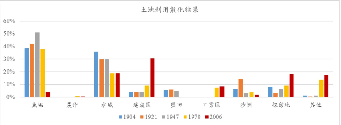
數化的年代分別有日治時期 1904 年、1921 年的地形圖及 1947-1948 年、1970 年代的歷史航 照影像，以及 2006 年第二次國土利用調查的成 果。土地利用數化結果直方圖如圖 5，其中魚塭 在 1970 年代之後大量地減少；農作區域歷年在 在此皆非常稀少；水域面積逐漸的減少，同時也 顯示陸域的增加；建成區域在 1970 年代後大量 攀升，成為全區佔地最大的土地利用類別；產業 土地利用上早期有開闢鹽場，而後來則設立工業 區；沙洲量 1921 年後逐漸減少；裸露地在 1921 年後則增加；其他在 1970 年代後大幅增加，不 過有將近一半增加的面積為道路使用土地。

4.3 土地利用變遷分析

由於本研究之時間軸跨越百年，因此將土地

利用變遷依據當時歷史背景及圖資種類分為三 個時期做討論，第一時期為 1904-1946 年，屬日 治時期；第二時期為 1947-1970 年代，為光復後 至工業起飛的 1970 年代；第三時期則為 1980 年 至今。

透過土地利用轉移矩陣的結果顯示了三個 時期各土地利用類別轉變的情形，表 5 為第一至 第二時期轉移矩陣的結果，其中變化最大者為由 水域轉為工業區的土地，顯示工業區有很大的面 積是填水為陸而成；而第二至第三期的轉移矩陣 結果如表 6，由表中可得知原本占最大宗的魚塭 用地今大幅減少，並且自 1970 年代開始魚塭是 由大量的被建築用地所取代。

為了能更清晰的了解各時期之時間變遷，我 們利用展示不同時期相同地方之時空資訊並對 應至歷史事件來進一步分析，而歷史事件之發生 時間則參考自 1998 年安平區志(林朝成及鄭水萍，

1998)之歷年紀事。

圖 5 土地利用數化結果直方圖

表 5 1904-1970 年代土地利用面積轉移矩陣(單位：公頃)

表 6 1970 年代-2006 年土地利用面積轉移矩陣(單位：公頃)

4.3.1 水域變遷

圖 6 中顯示台南運河的歷史變遷，在 1902 年舊運河潰堤後，由 1904 年的堡圖中我們仍可 發現舊運河的遺跡，是向北流入鹽水溪，大約是

今日民權路四段之位置；而後日本人於 1922 至 1926 年在籌足經費後開鑿之新運河則是向南流 經安平舊聚落的南方；到了第二時期，在經過運 河疏濬的工作，將運河連通至海，並且在 1949-1969 年間有建安客輪載客的功能，讓居民 能透過船隻往返安平至台南之間；第三時期，運

江若慈、曾義星:以時空資訊探討百年來台南古都沿海地區的土地利用變遷 223

河的樣貌大致沒有轉變，不過此時運河已經沒有 載客的功能。

圖 7 為港口之變遷，對沿海地區而言港口為 一項重要的設施，原本位於北方之安平舊港由於 逐漸淤積而失去港口機能，政府在 1974 年至 1979 年間於原鯤鯓湖興建新港口，位在安平舊港 南方兩公里處，因港口之興建造成漁光島被分為 南北兩部分，北部改為隸屬安平區的漁光里，

2001 年至 2008 年政府又重建安平舊港，並且在 此成立安平港歷史風貌園區，因此，今日我們可 看到安平南北有兩港的存在。

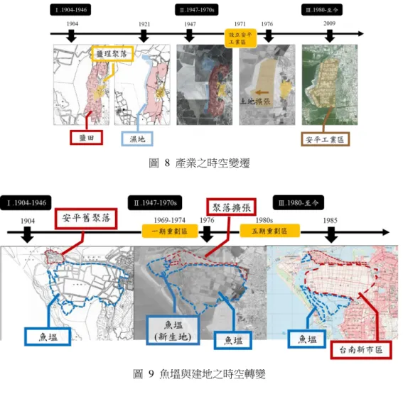
4.3.2 產業變遷

在產業方面的變遷如圖 8，由 1904 年的堡圖 中可知早期於鹽埕聚落旁開闢了一片鹽田，而在 1921 年至 1947 年間鹽田外的濕地增加，但隨著 經濟轉型，政府於 1971 年在原本的鹽田外填水 為陸，向外擴張土地並且設立安平工業區，而此 舉導致鹽田無法再運作而消失，導致產業的轉 變。

4.3.3 聚落變遷

圖 9 顯示魚塭地與聚落間之時空變遷，早期 安平舊聚落為位於北方的一個小聚落，大部分的 土地作魚塭使用，養殖虱目魚供府城消費，根據 日治時期之官方統計效忠里之魚塭有高達五百 餘甲(曾品滄，2012)，與數化結果相符；第二時 期的 1969 年至 1974 年間由於一期重劃區的設立，

使得安平舊聚落沿著運河向外延伸，此時魚塭面 積仍不斷增加；然而第三時期在 1980 年代後，

政府於安平規劃五期重劃區，將填魚塭填平為陸 地，大量的魚塭地轉變為台南新市區土地，因此 魚塭地大幅縮減，並且市政府也遷於安平區，成 為台南市政中心。

隨著聚落的擴張，人口亦快速的增加，根據 日治大正 14 年(1925 年)國勢調查結果表之記載 (台湾総督官房臨時国政調査部，1927)及安平戶 政事務所截至 2013 年官方資料(安平戶政事務所，

2014)顯示，在過去近 90 年間安平人口由不到六 千人增長至六萬餘人，安平各里之範圍亦不斷地 調整，並且最高人口密度分布也由安平舊聚落往 台南新市區移動。

圖 6 台南運河之時空變遷

圖 7 港口之時空變遷

圖 8 產業之時空變遷

圖 9 魚塭與建地之時空轉變

5. 討論

本研究為了能探討研究區域中百年來土地 利用在各時期之變遷，相較於過去其他探討變遷 研究之文獻建立時間序列更長且完整之圖資，其 地圖及歷史航照影像之精度雖未能與現代高精 度之影像相比，但對於長期土地利用大幅轉變之 呈現與分析，相信此精度已符合長期變遷之研究 需求，亦能彌補早期之文獻不足，在本研究中也 作為歷史事件佐證之資料。

然而在土地利用變遷分析上，由於古地圖、

歷史航照影像自動化判釋較不易，本研究採用人 工數化來進行量化分析，需耗費較多時間與人力，

雖然在數化前已先建立各土地利用類別之數化 參考依據，但此數化成果仍受主觀判斷所影響。

6. 結論

本研究運用了百年的時空資訊，包含從日治 時期的古地圖、早期歷史航照、經建版地形圖、

以及現代影像，完成百年間土地利用的數化圖，

提供了過去土地利用變遷之量化資訊。百年時空 資訊在日治時期古地圖及美軍空軍航照之精度 大約可達十餘公尺，而 1970 年代經過空三之正 射影像精度可達約 2 公尺。根據土地利用量化之 研究結果顯示，該區域早期占最大宗的魚塭用地 今大幅減少，從土地利用轉移矩陣可得知自 1970 年代開始魚塭是由大量的被建築用地所取代，水 域、鹽田及沙洲的面積相較百年以前，亦有減緩 的趨勢，而歷年來農業用地在此區皆非常稀少，

在另一方面，裸露地、工業及其他用地自 1970 年代來則有增加的趨勢。

藉由百年時空地理資訊的建立可以讓過去

江若慈、曾義星:以時空資訊探討百年來台南古都沿海地區的土地利用變遷 225

歷史事件更真實且更清晰地被描繪出來，相較於 以往的文史紀錄更清晰的呈現，並且能將其對應 至地理空間上，本研究顯示了時空資訊有助於長 期的變遷研究，也證明了多時期的時空地理資訊 為了解過去變遷的重要資料。

致謝

感謝科技部計畫(NSC 102 - 2627 - M - 006 – 001)的支持與經費的贊助，使本研究得以順利完 成。

參考文獻

丁志堅，2002。屏東平原土地利用變遷分析與模 式建立，國立台灣大學地理環境資源研究所 博士論文。

王超國，2009。以時間序列地圖分析臺江內海地 形變遷與演育，國立成功大學地球科學研究 所碩士論文。

內政部國土測繪中心，2014。http://lui.nlsc.gov.tw/

LUWeb/Welcome.aspx ( 取 得 日 期 2014/07/

24)。

台湾総督官房臨時国政調査部，1927。大正 14 年 国 勢 調 查 結 果 表 ， 国 立 国 会 図 書 館 。 http://kindai.ndl.go.jp/?__lang=ja ( 取 得 日 期 2014/01/21) 。

安平戶政事務所，2014。http://www.tainan.gov.tw/

anping/default.asp(取得日期 2014/03/17) 。 江正雄，廖泫銘，范成楝，張志君，林士哲，張

馨方，2006。運用空間資訊技術輔助歷史航 照影像地理空間標記處理模式之研究，2006 年臺灣地理資訊學會年會學術研討會，臺大 醫院國際會議中心。

林朝成，鄭水萍(主編)，1998。安平區志，安平 區公所。

林春吟，2012。日本植民地期台湾の地図に関す る研究－地図作製事業の検討を中心に，京 都大学人間‧環境学博士論文。

張文菘，2013。桃園地區土地利用變遷與影響因

素之空間分析，國立臺灣師範大學地理學系 碩士論文。

范毅軍，2006。 走進時光隧道：GIS 與時空資訊 的整合，中央研究院 2006 年八月知識饗宴。

莊育侃，2010。運用歷史航照與日治地形圖資料 探討花蓮地區之地形變遷，國立台北科技大 學土木與防災研究所碩士論文。

莊永忠，廖泫銘，范毅軍，2011。多源多期歷史 圖資於環境變遷分析之應用─以臺灣陳有蘭 溪集水區為例，2011 數位典藏地理資訊學術 研討會，台灣大學集思會議中心。

曾品滄，2012。塭與塘：清代臺灣養殖漁業發展 的比較分析，臺灣史研究，19(4)：1-47。

廖怡雯，2003。運用馬可夫鏈模式於台中市土地 利用變遷之研究，逢甲大學土地管理學系碩 士論文。

廖泫銘，江正雄，范毅軍，2011。臺灣航照影像 數位典藏成果與應用，國土資訊系統通訊，

78：57-72。

賴進貴，葉高華，2005。地圖概括化對環境變遷 研究之影響－以臺灣地圖資料為例，地理學 報，41：1-25。

蔡靜如，1998。台北盆地土地利用變遷趨勢之研 究，中興大學都市計劃研究所碩士論文。

Cardenal, J., Delgado, J., Mata, E., González, A., and Olague, I., 2006. Use of historical flight for landslide monitoring, 7th International Symposium on Spatial Accuracy Assessment in Natural Resources and Environmental Sciences, Lisbon, pp.129-138.

Clawson, M., and Stewart, C.L., 1965. Land use information: a critical survey of U.S. statistics including possibilities for greater uniformity, The Johns Hopskins Press.

Muller, M.R., and Middleton, J., 1994. A Markov model of land-use change dynamics in the Niagara Region, Landscape Ecology, 9(2):151-157.

Redweik, P., Roque, D., Marques, A., Matildes, R., and Marques, F., 2010. Triangulating the past-recovering Portugal's aerial images repository, Photogrammetric Engineering &

Remote Sensing, 76(9):1007-1018.

1Master, National Cheng Kung University

Received Date: May 25, 2015

2 Professor, National Cheng Kung University Revised Date: Aug. 26, 2016

*Corresponding Author, E-mail: [email protected] Accepted Date: Oct. 13, 2016

Land Use Changes of the Coastal Zone of Old Tainan City in the Past Hundred Years by Using Temporal Spatial Information

Jo-Tzu Chiang^1* Yi-Hsing Tseng²

Abstract

Temporal spatial information is considered as a favorable data source to comprehend the changes in the past.

Since 20th century, higher accuracy maps and images based on the technique of surveying has appeared in Taiwan. However, in order to retrieve these spatial information from the historical images, image registration and rectification should be done. In this study, we present a methodology of processing multi-temporal datasets during the past hundred years by commercial software (SOCET GXP 4.0) and a block adjustment with affine transformation. The temporal datasets used in this study include: (1) 1904 and 1921 ancient topographic maps;

(2)1947,1948 and 1970s historical aerial images; (3)1985-1989 economic planning and development topographic map; (4) 2009 satellite images; (5) 2010 ortho-images. The accuracy was also assessed. And we focused on the coastal zone of old Tainan city (about Anping nowadays). The land use are classified into 9 categories by manual interpretation and digitization on the temporal datasets. A transition matrix is also utilized to present the land use changes referring to some historical records.

Keywords: land use changes, temporal spatial information, coastal area, anping

航測及遙測學刊 第二十一卷 第 4 期 第 227-237 頁 民國 105 年 12 月 227

Journal of Photogrammetry and Remote Sensing Volume 21, No.4, 2016, pp. 227-237

DOI：10.6574/JPRS.2016.21(4).2

1 Master, Department of Geomatics,National Cheng Kung University Received Date: Apr. 08, 2013

2 Professor, Department of Geomatics,National Cheng Kung University Revised Date: Sep. 19, 2016

* Corresponding Author, E-mail: [email protected] Accepted Date: Dec. 23, 2016

Cloud Removal from Satellite Images Using Integrated Information Reconstruction

Kang-Hua Lai¹ Chao-Hung Lin^2*

Abstract

Cloud covers present in optical satellite images generally limit the data usage and increase the difficulty of data analysis. Information reconstruction of could-contaminated images thus plays a fundamental step in data preprocessing. A method to accurately and consistently reconstruct information of cloud-contaminated pixels in multitemporal remote-sensing images is proposed in this study. By utilizing temporal correlation of multitemporal images, a patch-based information reconstruction that spatiotemporally segments a sequence of images into several patches with similar temporal variation is performed, and then information from cloud-free and high-similarity patches is cloned to their corresponding cloud-contaminated patches. In addition, a seam passing through homogenous regions is determined for a cloud-contaminated region to reduce radiometric inconsistency. A cloud-contaminated region is segmented into several patches and their corresponding cloud-free patches are determined by a quality assessment index, and the multi-patch information cloning is solved by an optimization process with a determined seam. These processes enable the proposed method to accurately and consistently reconstruct missing information in cloud areas. Qualitative analyses on sequences of images acquired by the Landsat-7 ETM+ sensor and a quantitative analysis on a simulated data are conducted to evaluate the proposed method. The experimental results the ability of our method to generate visually smoothing reconstruction results.

Keywords: cloud removal, information reconstruction, optimal seam determination, poisson equation

1. Introduction

With the development of remote–sensing equipment, satellite images have drawn attentions and have been used in many fields such as geology, agriculture, meteorology, and regional planning. The satellite sensors can provide data for various applications. However, the images acquired by passive remote sensing sensors generally limited by the cloud covers. The limitation of passive remote sensing sensors is their sensitivity to weather conditions during data acquisition. For instance, the earth is on average about 66 % cloud covered and the land scenes are on average approximately 35%

cloud-covered globally (Ju and Roy, 2008). This phenomenon of cloud covers significantly reduces the availability of cloud-free optical satellite observations.

This study addresses the issue that clouds obstruct land covers, thereby resulting in missing data obtain from passive image sensors.

If multi-temporal images are available, the cloud-cover problem may to be eased by reconstructing the information of cloud-contaminated pixels. Data analysis such as classification of land

covers generally requires a cloud-free image composed of several patches acquired at different times and different conditions. These different conditions cause the relationships between land-cover classes and pixel intensities to vary over a data acquirement period. Thus, the naive approach that replaces cloud-contaminated pixels by their corresponding cloud-free pixels and then linearly adjust intensity values of replaced pixels has been proven inappropriate when the conditions of data acquirement changes significantly (Lin et al., 2013).

Lin et al. (2013) and Tsai and Lin (2016) proposed a nonlinear scheme instead of the linear intensity adjustment scheme to mathematically formulate the reconstruction problem as a Poisson equation and then solve the equation using a global optimization process. In addition, instead of reconstructing information pixel-by-pixel (Melgani, 2006;

Benabdelkader et al., 2008), which may contain radiometric inconsistency, the authors proposed a patch-based scheme to ease this inconsistency problem. This method can yield good cloud-free results; however, it is sensitive to boundary conditions when solving the Poisson equation, and also sensitive to the quality of patch selection. To address the problems above, this study proposes a

seam determination approach to select a seam passing through homogenous regions for providing good boundary conditions in reconstruction optimization.

In addition, by utilizing temporal correlation, a segmentation algorithm is proposed to segment a cloud-contaminated region into several patches with similar temporal intensity variations.

2. System Workflow and Review

2.1 system workflow

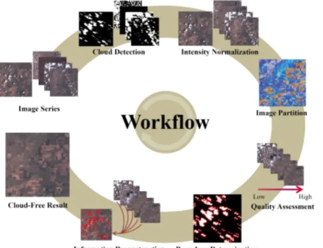
Figure 1 schematically illustrates the processes of the proposed method which consists of six main steps: cloud and cloud-shadow detection, image intensity normalization, multitemporal image segmentation, image quality assessment, seam determination, and information reconstruction. In the first step, a semi-automatic cloud detection approach is adopted to detect clouds and cloud shadows in the input images. In the next step, a linear image intensity normalization process is performed to achieve consistency in dynamic range of the input images. Next, the input images are partitioned into several patches with similar temporal variations while the input images are sorted according to the image similarity and the amount of clouds. In the step of seam determination, an optimization process using dynamic programming is performed to search for a seam in a cloud-contaminated region, and then the proposed information reconstruction algorithm is performed to recover the missing information of a cloud-contaminated region by solving a Poisson equation with the obtained seam as the boundary conditions.

Figure 1 Workflow of the proposed information reconstruction method

2.2 Review of Information Cloning Technique

The proposed approach is inspired by the concept of image editing presented by Pérez et al.

(2003) and is an extension of the information cloning proposed by Lin et al. (2013, 2014). The details of selected patches are used to reconstruct the information of corresponding cloud-contaminated regions in the target image. Instead of correcting the radiances and locally smoothing the boundaries of the cloud-contaminated regions or reconstructing the information pixel by pixel, the problem is mathematically formulated as a Poisson equation and then solved using a global optimization process.

Given a cloud-contaminated image, called target image and denoted as 𝐼𝑇, and a set of corresponding images captured at the same position but on different dates, called reference images and denoted as . The cloud-contaminated region in target image 𝐼𝑇 is denoted as Γ , and its boundary is denoted as ∂Γ . The information of cloud-contaminated pixels in target image 𝐼𝑇 are reconstructed by utilizing the reference images

. Let 𝑓 be an unknown image intensity function defined over the cloud-contaminated region Γ (i.e., the unknown that is to be calculated), 𝑓^∗ be the image intensity function defined over target image 𝐼𝑇 minus the cloud-contaminated region Γ, and V be a guidance vector field defined over Γ. The guidance vector field 𝐕 is defined as the gradient of the selected patches, and is used to guide the reconstruction process to optimize the pixel intensity values in the cloud-contaminated regions. To find an accurate and optimized reconstruction result (i.e., the solution of the unknown function 𝑓), the problem is formulated as an optimization equation with the Dirichlet boundary condition 𝑓|∂Γ= 𝑓^∗|_∂Γ as follows.

min𝑓∬ ‖∇𝑓 − 𝑉‖_Γ ² with 𝑓|𝜕Γ= 𝑓^∗|𝜕Γ ………...(1)

where

     x ,   y 

is the gradient operator.

Eq. (1) aims to derive the result 𝑓 with a gradient that is as close to the guidance vector field 𝐕 (i.e., the details of the selected patches) as possible.

The solution to (1) is the unique solution of the following Poisson equation with Dirichlet boundary conditions:

Kang-Hua Lai, Chao-Hung Lin：Cloud Removal from Satellite Images Using Integrated Information Reconstruction 229

∆𝑓 = div𝐕 over 𝚪 with 𝑓|𝜕Γ= 𝑓^∗|𝜕Γ ………..….(2)

where ∆=_𝜕𝑥^∂2₂+_𝜕𝑦^∂2₂ is the Laplacian operator, and

div𝐕 =^𝜕𝑣_𝜕𝑥¹+^𝜕𝑣_𝜕𝑦² is the divergence of the vector field 𝐕 = (𝑣1, 𝑣2).

Eqs. (1) and (2) are the fundamental formulations of information reconstruction proposed in Lin et al. (2013). These two equations aim to derive the result 𝑓 with a gradient that is as close to the guidance vector field V as possible under the Dirichlet boundary condition 𝑓|𝜕Γ= 𝑓^∗|𝜕Γ. The Dirichlet boundary condition is used to enforce the boundaries 𝜕Γ of the scalar functions 𝑓 and 𝑓^∗ to be radiometric consistency. The equation minimization indicates that the gradient of the unknown function 𝑓 is close to the guidance gradient field of the selected patch. The physical meaning is to fix the boundary intensity𝑓|𝜕Γ= 𝑓^∗|𝜕Γ

and interpolate inward while enforcing the spatial variations of the unknown function 𝑓 to the guidance vector field V as close as possible.

Therefore, this minimization has a good probability of consistently and accurately cloning the details of selected patches to the cloud-contaminated regions, when a suitable Dirichlet boundary condition and an accurate guidance vector field are given.

In this study, to improve the quality of information reconstruction, a spatiotemporal image segmentation approach is proposed to select cloud-free and high-quality patches and determine a suitable gradient guidance vector field V, and a boundary determination approach is proposed to select a suitable cloud boundary for providing a suitable Dirichlet boundary condition 𝑓|𝜕Γ= 𝑓^∗|𝜕Γ. Besides, an intensity constraint is included in the optimization of information reconstruction to alleviate error propagations.

3. Methodology

3.1 Cloud and Cloud-Shadow Detection

A semi-automatic approach is adopted to detect clouds and cloud shadows. The approach presented by Huang et al. (2010) is performed first, and then a simple user interface is provided for users to manually refine the detection results. In the automatic detection phase, relying on the physical fact that

clouds are bright and cold in the thermal band, a thresholding-based approach is adopted to detect clouds in the spectral-temperature space. Once the cloud pixels are extracted, their shadows are roughly predicted according to the cloud location and the solar illumination direction. The dark and connected components within the neighborhood of the predicted shadows are identified as the shadow components.

This approach is simple and can detect most clouds and cloud shadows. To robustly generate a cloud-free and cloud-shadow-free image, a manual refinement is further preformed to accurately determine the clouds and cloud shadows. In the proposed system, users are allowed to refine the cloud detection results through an interface with simple selection and morphological operations.

3.2 Spatiotemporal Segmen- tation

To select a suitable guidance vector field, that is, V in (1), for accurate information reconstruction and to handle clouds in a heterogeneous landscape, a spatiotemporal segmentation approach is proposed to segment the target image into several patches with similar temporal variation. A temporal variation map 𝑀_var is generated according to pixel intensity variations that occur in a defined period of time. The temporal variation of pixel (𝑖, 𝑗) is defined as the average intensity variation in the sequence of the target and reference images, that is, it is formulated as:

𝑀

_var

(𝑖, 𝑗) = ∑ (

^(𝐼_{𝑁𝑢𝑚𝐷𝑎𝑦(𝐼}^{𝑘+1(𝑖,𝑗)−𝐼𝑘(𝑖,𝑗))2}

𝑘+1,𝐼_𝑘)

)

𝑅𝑛

𝑘=1

…..(3)

where 𝑁𝑢𝑚𝐷𝑎𝑦(𝐼𝑘+1, 𝐼𝑘) is a function that returns the number of days between the acquiring dates of images 𝐼𝑘+1 and 𝐼𝑘, and there are 𝑅𝑛+1 images, including the reference and target images, used in the variation map calculation. Note that the cloud-contaminated pixels are excluded in the calculation of (3) since the information of these pixels is missing.

In the next step, the temporal variation map is partitioned into several patches in which each patch has similar temporal variations, meaning that each patch probably belongs to a landscape. Any image segmentation technique can be used here. For simplicity, the efficient and commonly-used k-means clustering method (MacQueen, 1967) is adopted.

With an initial set of k means, this method adopts an iterative refinement strategy to group the data into k classes {𝑠1, … , 𝑠𝑘} by minimizing the within-cluster sum of squares:

arg min_𝑠∑^𝑘_𝑖=1∑_{𝑥𝑗∈𝑠𝑖}‖𝑥_𝑗− 𝜇_𝑖‖²

……….…

.(4) where 𝜇𝑖 is the mean of pixel intensity values in class 𝑠𝑖.

From the generated temporal variation map, we can find that the croplands have a high temporal variation and the mountain areas have a low temporal variation which meets the expectation. In addition, the different landscapes are separated into different groups after applying the segmentation algorithm to the variation map, which enables the approach to handle clouds in a heterogeneous landscape.

3.3 Image Quality Assessment

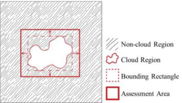
Once the cloud-contaminated regions as well as the target image are partitioned into several patches, we select a cloud-free and high-similarity patch in the reference images for each cloud-contaminated patch by utilizing the partition results to aid the patch quality assessment. In this study, the standard quality assessment called root mean square error (RMSE) is used to estimate the patch quality over an assessment area and to select the cloning patch from the reference images. The assessment area is a bounding rectangle with an extra width for each cloud-contaminated patch, as shown in Figure 2.

Figure 2 Illustrator of working area for image quality assessment

By considering the heterogeneous landscape, for each cloud-contaminated patch, the RMSE index between the target and reference images is calculated for only the regions belonging to the group of this cloud-contaminated patch. In this manner, a suitable cloning patch can be selected by using only the grouped regions in quality estimation. Besides, the cloud amount is also considered in the patch selection.

For a reference image, if the amount of clouds in a patch is greater than a defined threshold (set to 80%

for all experiments), the patches will not be selected as candidates.

3.4 Seam Determination

To improve the reconstruction accuracy, a seam determination approach is proposed. The Dirichlet boundary condition in Poisson equation, i.e., 𝑓|𝜕Γ= 𝑓^∗|_𝜕Γ in (1), significantly affects the results of inward interpolation as well as the quality of information reconstruction. The detected clouds are the working area of information reconstruction, and that provide a non-optimal boundary condition for Poisson equation. We argue that it is better to use a seam passing though homogeneous regions for cloning information of patches to a cloud-contaminated region instead of using the detected cloud boundary directly (Lin et al., 2013). It is because that nonhomogeneous regions containing high-gradient content generally have low consistency in pixel intensity and gradient of multitemporal images. Using a seam passing through nonhomogeneous regions as Dirichlet boundary conditions in reconstruction may cause inaccurate inward interpolation and information reconstruction.

The proposed seam determination approach consists of three steps: search space determination, cost map generation, and optimal seam determination.

The first step is to determine a search space around the cloud-contaminated area. The second step is to generate a cost map that considering the relationship between the target and source images. The last step is to determine the optimal seam in the search space by using a dynamic programming method with the aid of cost map.

Figure 3 Illustration of seam determination. From left to right: original image containing clouds, search space marked by red, cost map, and obtained seam (red curve) displayed in the cost map and the original image, respectively

3.4.1 Search Space Determination

In addition to enforce the seam passing though low-cost regions, the seam must be close to the cloud mask. Besides, the extreme concaves are excluded from the search space to simplify the process of seam determination. To meet these two requirements, the morphological operations, dilation and erosion, are utilized to define a search space without extreme concaves. As shown in Figure 4, the search space is determined by iteratively applying the dilation

Kang-Hua Lai, Chao-Hung Lin：Cloud Removal from Satellite Images Using Integrated Information Reconstruction 231 operator to the cloud-contaminated region, and then

iteratively applying the erosion operator to the dilated region with a 3x3 structure element B.

B = [1 1 1 1 1 1

1 1 1]

………...………

….(5) Then, the eroded region is defined as the search space. The number of dilations and erosions is set to 10, meaning that the width of search space is about 10 pixels. Note that the cloud-contaminated pixels are excluded from the search space, and the cloning patches for the search space are selected using the quality assessment.

Figure 4 Illustration of Search space determination.

Left: cloud mask; middle: result of dilation; right: result of erosion. The eroded region (red region) is defined as the search space

Figure 5 Illustration of search space elongating. (a) Cloud mask and search space (the number in the search space represents the order in each one-pixel-width circle); (b) destination space; (c) alignment of search space; (d) elongation of search space

Besides, to facilitate the calculation of seam optimization, the search space is embedded to a

regular space with a rectangle shape. This embedding is achieved by iteratively stretching and elongating the eroded one-pixel-width circles to fit a rectangle, as shown in Figure 5. In the elongation, the intensity values of empty pixels are obtained by linearly interpolating that of the neighboring pixels in their one-pixel-width circle. This embedding is achieved by iteratively stretching and elongating the dilated one-pixel-width circles to fit a rectangle. In the elongation, the intensity values of empty pixels are obtained by linearly interpolating that of the neighboring pixels in their one-pixel-width circle.

Obviously, this regular search space can facilitate the seam optimization.

3.4.2 Cost Map Generation

A cost map defined over the search space is generated for seam optimization. We propose that the seam is better to pass though homogenous regions in the target image and the seam is better to has similar gradient values in the target and reference images, i.e., consistent intensity values on the seam. Therefore, the cost map is defined as:

𝐶𝑜𝑠𝑡𝑀 = ∑(𝑖,𝑗)𝜖𝜔(‖∇𝐼_𝑇(𝑖, 𝑗)‖² + ‖∇𝐼_𝑇(𝑖, 𝑗) − ∇𝐼𝑅(𝑖, 𝑗)‖²)…………(6)

where ∇𝐼𝑇(𝑖, 𝑗) and ∇𝐼𝑅(𝑖, 𝑗) represent the gradients of target and reference images, respectively, at position (i, j); 𝜔 is the search space defined.

3.4.3 Optimal Seam Determination

The optimal seam is determined using dynamic programming with the aid of cost map. Dynamic programming is one of popular methods to solve a complex optimization problem, and that was proposed by Bellman (1954). The main idea of this method is tracing the path from start to terminal and has optimal cost, as shown in Figure 6.

By viewing the pixel intensity values in the cost map as the costs for a seam to pass through, the minimal-cost seam passing through the low-cost regions is obtained in the following manner. We define the function ^𝐶min^(𝑖,𝑗) as the cumulative minimum cost to reach the pixel (i,j) in the search space, and the cumulative minimum cost 𝐶min for all possible seams are computed as follows:

𝐶_min^(𝑖,𝑗)= 𝐶𝑜𝑠𝑡(𝑖, 𝑗) + 𝑀𝑖𝑛(𝐶_min^{(𝑖−1,𝑗+1)}, 𝐶_min^{(𝑖−1,𝑗)}, 𝐶_min^{(𝑖−1,𝑗−1)})… … … ..(7) In the end, the minimum value of the last row in 𝐶min indicates the end of the minimal-cost seam, and

thus, we trace back to the first row to find the optimal seam as well as the best boundary condition in information reconstruction. A result of seam determination is shown in Figure 7.

Figure 6 Illustration of dynamic programming

Figure 7 Example of seam determination

3.5 Information Reconstruction

While the information cloning approach proposed by Lin et al. (2013) yields good reconstruction results for most cases, it should be noted that the process of interpolating inward prorogates errors from the boundaries to the center of cloud-contaminated region may lead to an unnatural result, especially for the reconstruction with a high-cost seam. To solve this problem, a pixel intensity constraint is included in the optimization to balance fitting the guidance vector field V and linearly replacing pixel intensity according to that of the selected cloning patch. Including this intensity constraint, the optimization in (1) is reformulated as:

min𝑓∬ (‖∇𝑓 − 𝑉‖_Γ ²+ (𝑓 − 𝑓𝑐𝑝′)²) … … … . …(8) with 𝑓|𝜕Γ= 𝑓^∗|𝜕Γ

where 𝑓𝑐𝑝 is the intensity function defined over the

selected cloning patch, and 𝑓𝑐𝑝′

is the intensity adjustment result of 𝑓𝑐𝑝, which is calculated by (2).

In the implementation, Eq. (8) is discretized by a pixel grid. Let 𝑁𝑝 be the pixel set of the 4-connected neighbors for a pixel p in target image 𝐼𝑇, and denote <p, q> as a pixel pair, such that pixel q is one of the 4-connected neighbors of pixel p (i.e., 𝑞 ∈ 𝑁𝑝).

Let 𝑓(𝑝) be the value of the image function f at the position/pixel p. The task is to compute the pixel intensity values in the cloud-contaminated region Γ.

The discretization of (9) yields the following discrete optimization equation:

min_𝑓∑<𝑝,𝑞>∩Γ≠0|(𝑓(𝑝) − 𝑓(𝑞) − 𝑣_𝑝𝑞)²+ (𝑓(𝑝) − 𝑓^′(𝑝))²| ………(9)

with 𝑓(𝑠) = 𝑓^∗(𝑠) for all 𝑠 ∈ 𝜕Γ

where 𝑣𝑝𝑞= 𝐼𝑅(𝑝) − 𝐼_𝑅(𝑞), which is the guidance gradient of the reference image at position p.

4. Experimental Results and Discussion

Landsat-7 ETM+ images having various landscapes were used to test the feasibility and performance of our method. For simplicity, the 30 meter blue band (0.45-0.52 micron), green band (0.53–0.61 micron), red band (0.63–0.69 micron), and near-infrared band (0.78–0.90 micron) of ETM+

images were used only; the two mid-infrared, thermal infrared, and panchromatic bands were not used. We select four study sites including the Colorado in western USA, Taichung in western Taiwan, Taipei in northern Taiwan as shown in Table1.

The Colorado Landsat acquisitions, Jordan, and parts of Taiwan Landsat acquisitions having only a few cloud covers are suitable for conducing quantitative analyses using simulated clouds. The Taiwan Landsat acquisitions containing on average about 34 % cloud covers are suitable for testing the feasibility of our method. In the Taiwan Landsat acquisitions, the clouds and cloud shadows were identified using the unsupervised detection approach proposed by Huang et al. (2010) first, and then manually refined the detection by a simple user interface with selection and erosion operations. To estimate the quality of information reconstruction, the standard and commonly used measurement, root-mean-square error (RMSE), is adopted, and all the test data are displayed on 8-bit image.

Kang-Hua Lai, Chao-Hung Lin：Cloud Removal from Satellite Images Using Integrated Information Reconstruction 233

Table 1 Landsat ETM+ acquisitions for the study sites.

Site, country Site location (latitude, longitude)

Path/Row

coordinates Acquisition data Cloud cover rate Colorado, USA 37.442N,102.807W 32/34 1999/07/03 – 2003/05/27 6%

Taichung, Taiwan 24.195N, 120.658E 118/43 1999/11/19 – 2003/05/22 25%

Taipei, Taiwan 25.035N,121.494E 117/43 1999/08/08 – 2003/05/31 28%

4.1 Result of information reconstruction

The images containing homogeneous regions and intricate structure regions were tested to evaluate the proposed method. The data of mountain areas (homogeneous regions) is shown in Figure 8 and the data of urban areas (intricate structure regions) is show in Figure 9. In Figure 8, the top images are cloudy target image and four cloudy reference images whose acquisition dates are close to that of target image. The cloud-contaminated regions are masked first, and the partition maps of images are constructed by proposed method by using the parameter setting k=20. Then, the image quality assessment approach is utilized to select the best source and guidance vector function. Finally, the missing information is reconstructed through the solver of the refined Poisson equation with the aid of determined guidance vector and optimal boundary condition.

4.2 Information reconstruction of simulated cloud-contam- inated image

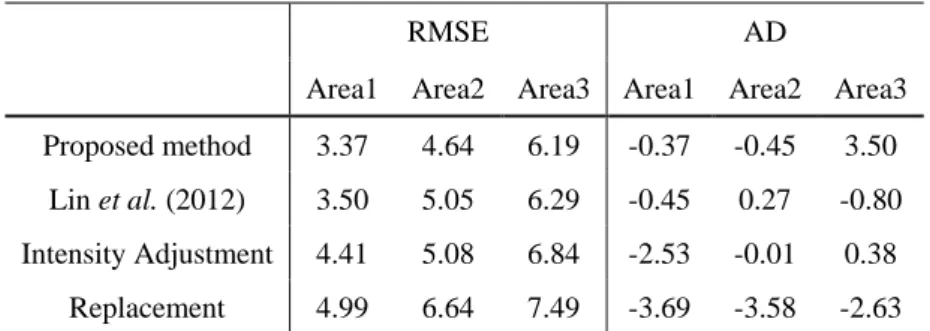
Reconstruction of simulated cloud-contaminated pixels was conducted to quantify reconstruction accuracy and to compare our method with the related methods. In this experiment, an image that contains

three simulated regions with different cloud contaminations was tested. The acquisition dates of target and reference images are March 3, 2003 and January 30, 2003, respectively. Area1 contains mountains; Area2 contains mountains and urban areas;

Area 3 contains mountains, urban areas, and croplands. Several related methods, including patch replacement, intensity adjustment suggested in (Li et al., 2003; Gabarda and Cristobal, 2007; Helmer and Ruefenacht, 2005; Tseng et al., 2008; Wang et al., 1999), histogram matching (USGS, 2004), information cloning method proposed by Lin et al.

(2013), and the proposed method were evaluated. To ensure fair comparison, only one reference image was used, and thus, the process of spatiotemporal segmentation is omitted from our method. In the method of intensity adjustment and histogram matching, information reconstruction is achieved by adjusting pixel intensity values according to a transformation function that is determined using mean and standard deviation of intensity values or histogram matching. In the approach of (Lin et al., 2013), the radiometric inconsistency is eased by error propagation. However, the reconstruction quality is sensitive to boundary conditions and selected cloning patches. In this study, seam optimization and spatiotemporal segmentation are adopted to optimize information reconstruction. Therefore, as can be seen in Figure 10, our result is closer to the actual image, i.e., the ground truth, compared with the results generated by related methods, indicating that better reconstructions are obtained.

Figure 8 Color composites of the temporal sequence over the Yangmingshan mountainous area in northern Taiwan. The images from mid-left to mid-right are cloud mask, partition map, source map and optimal boundary, respectively

Figure 9 Color composites of the temporal sequence over the Taipei in northern Taiwan. The images from mid-left to mid-right are cloud mask, partition map, source map and optimal boundary, respectively