Optical response of layers of embedded semiconductor quantum dots

(1)

Optical response of layers of embedded semiconductor quantum dots

C. M. J. Wijers and Jiun-Haw Chu

Department of Electronic Engineering and Institute of Electronics, National Chiao Tung University, 1001 Ta Hsueh Road, Hsinchu 300, Taiwan

J. L. Liu

Department of Applied Mathematics, National University of Kaohsiung, Kaohsiung 811, Taiwan

O. Voskoboynikov

Institute of Electronics and Department of Electronic Engineering, National Chiao Tung University, 1001 Ta Hsueh Road, Hsinchu 300, Taiwan

共Received 12 April 2006; published 19 July 2006兲

The influence of the surrounding semiconducting matrix upon the polarizability of embedded nanoobjects 共quantum dots兲 has been investigated. The previously proposed hybrid model has been extended to accommo-date the influence of embedding. It turns out that excess discrete dipoles having an excess polarizability against a uniform background identical to the dielectric host material build the basis for a modified discrete dipole model, suited to describe the optical response of this system. The individual dipoles are described by means of dielectric embedded oblate ellipsoids as to their static response. An efficient description of the electrostatics of these ellipsoids has been given in terms of explicit functions using cylindrical coordinates and compatible with similar derivations for spherical dielectric objects. The dynamic contribution, responsible for frequency depen-dence is determined quantum mechanically and added to the embedded bare polarizability. The result of the model for the particular InAs quantum dot GaAs host combination investigated is a slightly decreased internal reflectance as compared to vacuum and an overall strong increment of the absorbance, the structure in the reflectance and of the ellipsometric angles.

DOI:10.1103/PhysRevB.74.035323 PACS number共s兲: 73.21.⫺b, 75.20.Ck, 75.75.⫹a

I. INTRODUCTION

To make materials from at least two other materials 共el-ementary or compound兲 by changing the dimensions and ge-ometry of their interface is the essence of metamaterials re-search. Modern metamaterials research concentrates upon dimensions in the nanometer range. Especially the construc-tion of metamaterials based upon III-V semiconductor na-noobjects 共nanosized quantum dots, nanorings, etc.兲 is a promising field of research, particularly for its high potential to develop optical applications. The present quest for nega-tive refracnega-tive index materials1–3_{is a good example of such}

research opening a completely unorthodox field of optics. Negative refractive index metamaterials have been made in the frequency range up to THz,4but the building blocks of these metamaterials were mm sized. Smaller building blocks will be required to move the desired material characteristics to higher frequencies and semiconductor nano-objects are ideal candidates. This kind of research will need appropriate model descriptions to guide it. In the traditional use of nano-object based metamaterials for lasing applications the mod-elling focuses upon photoluminescence and spontaneous emission, but such modelling is not really adequate for metamaterials such as negative refractive index materials. Then a proper description of the basic linear optical proper-ties of these materials is a first necessity. In two previous papers we have addressed already some fundamental issues concerning this problem, but those papers treated only iso-lated nano-objects.5,6 _{The next step to make this model of}

real use is to put these nano-objects in a suitable host mate-rial. In other words, we want to know what happens with the

共linear兲 optical properties of the nano-objects upon embed-ding, and this is the question this paper wants to address for composite nano-object metamaterials.

We consider a metamaterial build from nano-objects of characteristic size a. For such a system we assume

␭ Ⰷ aL⬎ a,

where␭ is the wavelength of the electromagnetic wave and aL an average distance between the nano-objects in the metamaterial. We will start our treatment by explaining the difference between bare and dressed polarizabilities for the case of embedded nano-objects and consider the commonly known problem of the dielectric sphere in an external field. This sphere, as we will show, can be replaced by a discrete excess dipole and a corresponding excess polarizability. As a result an ensemble of these nano-objects can effectively be treated by means of modified discrete dipole theory, where frequency dependence enters the modelling through quantum mechanics, as treated before by the authors of this paper.6

The response of an embedded dielectric ellipsoidal nano-object is subsequently added to the description in order to model as closely as possible realistic semiconductor quantum dots. The resulting hybrid model will be used to treat the change in optical properties of semiconducting nanosized ob-jects 共InAs quantum dots兲 upon embedding in a foreign semiconducting host material共GaAs兲. Hybrid means for this model that we combine the discrete nonlocal description for the excess response of the dots with a local continuum de-scription for a uniform background, extending over the host material, but also over the dots. Temperature dependence

(2)

will not be taken into account, which means for this paper that the calculations will relate to the T = 0 K situation. Also aspects of nonlocal quantum mechanical interactions, since those involve typical surface effects which are ignored al-ready implicitly in the envelope function approximation, will be left out from consideration, although we have investigated those in detail in the past for different systems.7

II. THEORY

In this section we will derive the hybrid model we will use to describe the optical response of metamaterials com-posed of nano-objects like quantum dots, embedded in a di-electric host material共see Fig. 1兲. The nano-objects will be

assumed in this paper to have a dielectric constant⑀different from the dielectric constant⑀mof the host material.

In order to keep the paper more transparent we will use during the derivation of the model itself the more familiar and simpler dielectric spheres, to represent the nano-objects. The use of that representation allows for a stronger focus upon the main issue: the consequences of embedding upon the optical properties of an ensemble of nano-objects, in this case a square lattice of quantum dots. For the actual calcu-lations, as told before, flat oblate ellipsoidal dielectric nano-objects will be used. A derivation of the required electromag-netic properties of these ellipsoidal bodies is given in the Appendix. This derivation is such that it can be joined smoothly with the spherical body treatment by replacing a minimum of characterizing parameters.

A. Bare and dressed polarizabilities of semiconductor nano-objects

Quantum dots are generally classified as artificial atoms. Therefore their optical response should also be described in an atomiclike fashion, e.g., by means of polarizabilities. Op-tics in combination with quantum dot structures relies either upon expressions for optical absorption8 _{or upon oscillator}

strengths,9,10 _{being the squared modulus of the optical}

tran-sition matrix element.11 _{The proper approach should be to}

use the Kramers-Heisenberg expressions, but it is not straightforward to apply those to the case of a dot, described

by means of envelope functions.6 _{This holds even more}

when we have to model embedded nano-objects by means of a hybrid description. Then it becomes necessary to distin-guish adequately between bare and dressed polarizabilities, although we have used those already implicitly in our previ-ous papers.5,6_{From Ref.}₆_{we summarize the important}

defi-nitions. The dressed polarizability␣Dis defined by

p =␣JDEL, 共1兲

where ELis the classical local field, which equals the exter-nal field EXfor the case of a single nano-object. This polar-izability is the polarpolar-izability which follows directly from ex-perimental observations, since the external field is measurable. The bare polarizability ␣B is defined with re-spect to the applied electric field EA by

p =␣JBEA,

EA= EL+ tIp, 共2兲

where t is the full electromagnetic selfinteraction tensor for the nano-object, to be called further intracellular transfer ten-sor. It is easily verified that for the case of a dielectric sphere or ellipsoid, the applied field equals statically the internal field. For that case it is also the average electric field. The bare polarizability␣Bis not measurable and the only way to obtain it independently is by means of theory. Further we repeat from Ref. 6 _{the elementary relationship between the}

two kinds of polarizability:

␣JD −1

=␣JB −1

− tI. 共3兲

The distinction between bare and dressed polarizabilities, al-though not always under these labels, is old and goes back to the discussion about the validity of the Sellmeier and Lorentz-Lorenz, Clausius-Mossotti descriptions.12,13_The

dis-tinction however is still relevant and here necessary even to understand properly the physics behind the hybrid method.

The key reason why for hybrid models the distinction between bare and dressed polarizabilities needs to be empha-sized concerns the fundamental issue to which static polariz-ability the dynamical contribution⌬␣, as derived before in6 FIG. 1. Conceptual picture of the building of a metamaterial from semiconductor nano-objects共embedded ellipsoidal quantum dots兲.

(3)

⌬␣共␻兲 =3 4 e2 បreh 2_共xˆxˆT + yˆyˆT兲

兺

l=0 −2 兩具Fhl兩Fel典V兩2fhl,el共␻兲共4兲 needs to be added. Our choice6_{has been to add it to the bare}

polarizability. On the other hand the expression of the polar-izability in Ref.5 which was used to derive共4兲 is definitely

a dressed one. As shown above it is all a matter of the elec-tric field with respect to which we define the polarizability. In Ref.5 the extension of the original Kramers-Heisenberg induction derivation to a corresponding polarizability was at stake. In the original Kramers-Heisenberg paper23_{the choice}

of the electric field was explicitly the external one. In that derivation the electric field comes out from the matrix ele-ment of the perturbation HˆD+ W, where W is the part of the perturbation due to the external electric field EX共in Ref. 5,

EX兲 and HˆDthe共dissipative兲 part due to the internal electric field EI.5In the original Hamiltonian关Eq. 共14兲 of Ref.5兴 the perturbation is governed by A being the unique microscopic vector potential and it is this potential which governs the transition strength’s involved. The concept of the polarizabil-ity requires a finite integration volume with the atomic vol-ume as its preferred minimum and uses therefore inherently approximate electric fields. In our view the electric field must be external to the quantum mechanics. Therefore we have chosen to define the theoretical quantum mechanical polarizability with respect to the electric field being closest to the microscopic one and that is the applied or average field as defined above. This choice agrees with the approach used in Refs.13–16. This choice will not change the expression of the polarizability as such, since it affects only the dissipative part HˆD and that is accounted for already by the Lorentz radiation damping term. For larger systems like a nano-object this does not mean that HˆDvanishes. There it becomes replaced by the electronic decay mechanisms like electron-electron or electron-electron-phonon interactions, but these are in-cluded phenomenologically through the choice of␥共␻兲, the imaginary part of the complex resonance frequency␻ˆlk be-tween states l and k.5 Therefore we will use for the bare embedded dynamical polarizability␣BE共␻兲 the expression:

␣BE共␻兲 =␣BE+⌬␣共␻兲, 共5兲 where⌬␣共␻兲 is the same as used before in Ref.6 and␣BE the bare embedded static polarizability.

B. The hybrid method for embedded dielectric objects

Bare and dressed polarizabilities are generic concepts. To show how they relate to realistic situations and what their specific expressions are, we begin by considering the static polarizability of a spherical body. From this specification we will learn how our hybrid method must be set up. As men-tioned already we will leave the case of the ellipsoidal di-electric bodies to the Appendix, but will use the results for the actual calculations.

⑀−⑀m ⑀+ 2⑀m

冊冉

R3 r3

冊

册

E0r cos␪. 共11兲 For the construction of the hybrid model the potential is not as useful as the electric fields, which we prefer to write as

(4)

冉

⑀−⑀m

⑀+ 2⑀m

冊

, 共14兲

where the excess character is clear from the difference be-tween⑀and⑀min the numerator. When ⑀happens to equal

⑀m, there is no excess dipole strength. The nano-object is still polarized then, but no more than its surroundings. The outer field共12兲 can be rewritten now as

EO共r兲 = E0+ 1 ⑀m t I共r兲p t I共r兲 =3rˆrˆ T − 1 4␲⑀0r3 , 共15兲

where t共r兲 is the vacuum static transfer kernel from discrete dipole theory.

We can proceed using these rewritten equations to handle systems with more embedded nano-objects. This extension requires no more but the systematic replacement above of the external field E0by the local field EL, as follows:

ELi= E0+ 1

⑀m

兺

i⫽j

t

Iijpj, 共16兲

where tij is the vacuum intercellular transfer tensor, where the presence of the index ij indicates intercellular character in the notation of this paper. The induction for the excess dipole strength’s pibecomes

pi=␣Ji

冉

E0+ 1

⑀m

兺

i⫽j

t

Iijpj

冊

, 共17兲 where we return to the dynamic equations by using for tijthe frequency dependent expressions. We see that although we started our treatment of the embedded dielectric spheres as an exercise in macroscopic dielectric continuum theory, the final result can be directly interpreted as an effectively dis-crete description. This remark builds the essence of the hy-brid method. The system of equations to be solved becomes

␣ Ji−1pi− 1 ⑀m

兺

i⫽j t Iijpj= E0, 共18兲 where␣iis the excess polarizability defined above共14兲. Here some comment should be given about the influence of the embedding medium upon the polarizability and transfer ten-sor, commonly called “screening.” If we understand screen-ing of a certain quantity as its division by ⑀m of its un-screened 共vacuum兲 value, then definitely the embedded transfer tensor is screened. This is remarkable, since at first inspection of the result共12兲 it looks as if there is no

screen-ing at all. It is not possible to say whether the polarizability is screened. Again, at first glance it looks as if the⑀min front of the expression for the polarizability共14兲 is there because

of screening. Such interpretation however violates what we have just written about screening. Since the polarizability here is an excess one, there is no properly defined vacuum value to refer to. We return to this point in the next section. A next question concerns the external field E0, in the sense of the field applied to the dipole. When the sphere is surrounded by vacuum this field is the external field and it is clear what is meant by that. When the sphere is surrounded by a medium, we have from the result above as an immediate answer that what we have to call here the external field, is the macroscopic (average) field inside the surrounding me-dium far from the nano-object. From this definition it is clear that the excess polarizability共14兲 is a dressed polarizability.

We determine now the bare and dressed 共excess兲 static polarizabilities for the case of embedded ellipsoidal nano-objects as derived in the Appendix. At forehand we mention already that dressed has nothing to do with screening. Nano-objects either in vacuum or embedded have both dressed and bare polarizabilities, all being different. The dressed embed-ded polarizability␣_DEcan directly be taken from the Appen-dix, since the analogy with the dielectric sphere is obvious,

␣DE,u=⑀0V

冉

⑀m共⑀−⑀m兲 ⑀m+ Nu共⑀−⑀m兲

冊

Nz= 1 1 −␨2

冉

1 − ␨cos−1␨

冑

1 −␨2

冊

共ellipsoid兲, Nz=1₃ 共sphere兲, Nx= Ny= 1 − Nz共␨兲 2 , 共19兲

where u = x , y , z. We prefer to classify this result as local electromagnetic. The bare embedded polarizability ␣BE fol-lows from a reorganization of the expression for␣DE:

␣DEu=

␣BE 1 − tEu␣BE

,

␣BE=⑀0V共⑀−⑀m兲, 共20兲 where we see that␣BEis an excess quantity too, but it is also not screened. This reorganization yields further the intracel-lular embedded transfer tensor tE which brings in the

(5)

elec-tromagnetic interactions taking place inside the nano-object, opposite to the intercellular transfer tensors which account for the electromagnetic interactions between nano-objects. Therefore we will classify this result as nonlocal electromag-netic. The embedded intracellular transfer tensor tE is for ellipsoidal bodies given by

tEu= 1 ⑀m tu, tu= − Nu ⑀0V + ik 3 6␲⑀0 , 共21兲

where t is the corresponding tensor for the vacuum situation. For embedded nano-objects the intracellular transfer tensor

tEis screened by⑀m, the dielectric constant of the embedding medium. For a nano-object in vacuum the intracellular trans-fer tensor t is, in contrast, not screened by the dielectric constant⑀of the nano-object. The dressed polarizability de-pends on the bare polarizability and on the intracellular transfer tensor. Only that tensor is screened in the case of embedding and only through the influence of that tensor screening enters the dressed embedded polarizability. By it-self it is strange that the intracellular transfer tensor happens to be screened by the surrounding ⑀m, but the derivation leaves no other choice. All that can be said to understand it, is that we are dealing with an excess polarizability and not with a full polarizability.

We investigate in detail the behavior of the dressed and bare polarizability. Using the definitions collected in共19兲 it is

easy to give an explicit relation for the ratio between␣Dand

␣B,

冉

␣D ␣B

冊

= ⑀m ⑀m+ Nu共⑀−⑀m兲 . 共22兲

For the case of the dielectric sphere this ratio has been plot-ted in Fig.2as a function of the dielectric function⑀of the nano-object. For free nano-objects, the vacuum case, the ra-tio is shown by the dashed line. For semiconductors ⑀ is large, above 11, and the bare polarizability is at least 4 times

larger than the dressed one. Embedding changes all this. For the case of GaAs we have⑀m= 13.1 and the dressed to bare ratio is shown by the solid line. Then for embedded semi-conductor nano-objects, there is hardly any difference left anymore between the dressed and bare polarizability.

For the oblate ellipsoid-type of nano-objects to be treated further on, the dressed to bare ratio is plotted in Fig.3. For that case the consequences of embedding upon the ratio are even more outspoken. When we use for the dielectric con-stant of the nano-object the value⑀= 15.15,18_{the ratio}_␣

D/␣B increases by a factor of 11.9 for the z component and by a factor of 1.8 for the x component. So the increments caused by embedding are highly anisotropic. For values of⑀below

⑀m共⑀⬍13.1兲 this results even in a reversal of the anisotropy. For InAs there is not yet reversal, but the anisotropic incre-ment of the dressed polarizability results into an almost dis-appearance of the externally observable anisotropy. The ratio

␣D/␣Bis for that case 0.878 for the z direction and 0.991 for the x direction. The consequences are twofold. First the dif-ference between dressed and bare polarizability is almost gone. Next the anisotropy has almost vanished. Both phe-nomena have the same origin. In the expression for the dressed polarizability the influence of the intracellular trans-fer tensor t has been severely weakened by the⑀m. Since this tensor is responsible in the nonlocal description for both the dressing and the anisotropy共the bare polarizability is isotro-pic兲, it explains both effects.

C. Electromagnetic response

The calculation of the optical response of an embedded square lattice of nano-objects can be performed using the same共Vlieger兲 expressions19,20_{for the reflected and}

transmit-ted electric fields from a square lattice with lattice constant aL, as used before in Ref.6 共we leave out transmittance’s兲: FIG. 2. ␣_D/␣_Bfor a sphere as a function of its dielectric

con-stant⑀. Shaded, semiconductor regime. _{tric constant}FIG. 3.␣D_{⑀. Shaded, semiconductor regime. The two upper}/␣Bfor an oblate ellipsoid as a function of its dielec-curves are for ⑀m= 13.1, the embedded case, and the two lower

curves are for⑀m= 1, the vacuum case. x共dashed兲, z 共solid兲

(6)

rss= fk Aycos␪i− fk , rpp= fkcos␪i Ax− fkcos␪i − fksin 2_␪ i Azcos␪i− fksin2␪i . 共23兲

The following abbreviations are used to make the expres-sions more concise, but they contain also all elements which change, when the nano-object gets embedded:

Au=␣0␣BEu共␻兲−1− 1

⑀m

共fu

⬘

+ tu兲,

fk= 2␲iaLkm, 共24兲 where u is x , y , z and␣₀= 4␲⑀₀a_L3. We use here the bare ex-cess polarizability 共21兲, since we combine the intracellular

transfer tensor t with the planar transfer tensor f Refs.21and

22 关see also 共3兲兴. Both tensors are made dimensionless

through f =␣0f and t =␣0t. All transfer tensors are screened, as described before. An overview of the numerical procedure to determine the dipole strength p and through that of the optical response is shown in the diagram of Fig.4. The wave number kmchanges also upon embedding, as will be treated next. Although externally only dressed polarizabilities are observable, the entire theoretical derivation makes only use of bare polarizabilities which definitely improves the trans-parency of it. Effectively the bare polarizabilities turn into dressed ones through the intracellular transfer tensor t but

this tensor is added only at the last stage, when the Vlieger equations are invoked.

Since the Vlieger equations are dynamical they contain the wave number k, which is directly affected by the dielec-tric constant ⑀m of the embedding medium, because it fol-lows from the dispersion equation for the embedding me-dium:

ⵜ2_{E −}_⑀ 0␮0⑀m

⳵2

⳵t2E = 0.

We refer to the wave number inside the medium as kmand to the vacuum wave number as k0=␻/ c. The result becomes

km=

冑

⑀m

␻

c =

冑

⑀mk0.

The embedded wave number km turns out to be almost 4 times共3.89兲 as large as the vacuum wave number k0for InAs and affects the reflection coefficients by the same amount, as can be seen from Eq.共23兲.

III. NUMERICAL RESULTS

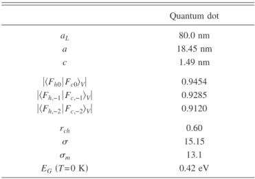
We show the results of the influence of embedding upon the optical response of an embedded square lattice of nano-objects for the case of quantum dots. We use the same InAs/ GaAs-quantum dots and lattice configuration as stud-ied in Ref. 6 The dots are statically modelled by oblate di-electric ellipsoids with a , c as the long, respectively, short axis. The relevant data are given in TableI. For further de-tails we refer to Ref.6.

The bare polarizabilities of this system are given as

␣Bx共␻兲 =␣By共␻兲 =␣B+⌬␣共␻兲,

␣Bz共␻兲 =␣B, 共25兲 where ␣B is as given by the second line of Eq. 共20兲. The addition of the dynamical⌬␣共␻兲 restores the anisotropy as we will discuss later. We compare these static bare embedded 共excess兲 polarizabilities␣BE to the vacuum bare polarizabil-ity␣BVof the same quantum dot,

FIG. 4. Flow diagram of process steps to arrive at reflection and transmission for an embedded monolayer of nano-objects. Transfer tensors f⬘, t are for vacuum. Susceptibility␹=⑀−1.

TABLE I. Basic input parameters for lattices of dots. For mean-ing of symbols see the text and Ref.6.

Quantum dot aL 80.0 nm a 18.45 nm c 1.49 nm 兩具Fh0兩Fc0典V兩 0.9454 兩具Fh,−1兩Fc,−1典V兩 0.9285 兩具Fh,−2兩Fc,−2典V兩 0.9120 rch 0.60 ␴ 15.15 ␴m 13.1 E_G共T=0 K兲 0.42 eV

(7)

␣BV= 4.672 45⫻ 10−3␣0,

orien-tation by an even larger amount. For the x orienorien-tation this factor is 1 and has hence no effect. The behavior in the z direction is entirely related to the electromagnetic interac-tions inside the nano-object and its screening. So both re-markable effects have the same origin: the screening of the intracellular transfer tensor.

The frequency dependent behavior of the x component of the bare polarizability ␣B is shown in Fig.5 and has been calculated using Eqs.共20兲, 共4兲, and 共5兲. We have used for the

dampingប␥= 5 meV. The z component of the bare polariz-ability␣B is constant according to共25兲 and has the value of

␣BE, hence

␣Bz= 6.769 27⫻ 10−4␣0. 共30兲 In the left-hand panel共a兲 of Fig.5we show the real part of the bare polarizability ␣Bx. This is the stronger component. For the free floating quantum dots 共vacuum embedding兲 there is just very weak structure in the real part as can be seen in the left-hand panel of Fig.5. The first strong effect of embedding for the real part is a decrement of the mean value by almost one order of magnitude. The reduction factor is given by 1 / gBand the value is 6.9. Simultaneously however the structure due to the quantum mechanical transitions is relatively enhanced. As can be seen from Eq. 共21兲 the

re-sponsible mechanism is the subtraction of the embedding dielectric constant⑀m. The addition of the dynamic quantum mechanical contribution⌬␣共␻兲 to only the x and y compo-nent restores the anisotropy, almost lost by the embedding. The picture is quite different for the imaginary part as shown in the right-hand panel 共b兲 of Fig.5. Since the embedding dielectric constant has no imaginary component in our region of interest, the only imaginary contribution is from ⌬␣共␻兲. As a result the imaginary part is not influenced by the em-bedding, as we see in Fig. 5, where the results for vacuum and embedding with⑀m= 13.1 coincide.

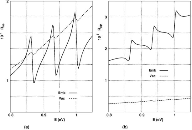
The first 共internally兲 observable optical response term is the reflectance. For a single monolayer these reflectance’s are weak. Embedding however does not deteriorate that situation much. For an angle of incidence of␪i= 60° the reflectance’s for the two polarization directions s and p are shown in Fig.

6. This angle is close to the Brewster angle, where s type of reflectance is always 共much兲 stronger than for p type. The left-hand panel共a兲 shows that there is only weakly decreased TABLE II. Dressed static polarizability␣Dfor x , z orientation

for vacuum and embedded situation.

Vacuum Embedded

␣Dx 2.583 09⫻10−3␣0 6.731 66⫻10−4␣0 ␣Dz 3.467 74⫻10−4␣0 5.966 24⫻10−4␣0

(8)

reflectance for the s component upon embedding. That this is correct can easily be understood. In the denominator of the Vlieger expression for rss, Eq. 共23兲 the dominant term is

␣0␣Bu−1. This dominance is so strong that approximately we have that

rss⬇ fk␣By

␣0cos␪i

. 共31兲

The bare polarizability␣By decreases by the factor gB being 0.145. This is compensated by the numerator fk which

in-FIG. 6. Reflectance R for angle of incidence␪_i= 60°.共a兲 R_ss,共b兲 R_pp. Dashed curves, vacuum共no embedding兲; solid curves, embedding with⑀m= 13.1.

FIG. 5. Bare polarizability␣x. 共a兲 Real part of ␣B,x/␣0, dashed curves, vacuum 共no embedding兲; solid curves, embedding with⑀m

(9)

creases with

冑

⑀mor 3.9, but the overall result is a decrement of about 0.6, in agreement with the calculations. For the p component the situation is different. There the embedded re-flectance is larger than the vacuum rere-flectance even up to a factor of 3, but also this is consistent. Roughly the arguments are the same as before for the s component, but now the second term in the expression for rppbecomes the dominant one. Then␣Bztakes over and we have mentioned already that this polarizability is larger than its vacuum counterpart. The result is a reflectance larger than for free floating quantum dots. The relevant contribution however is the one due to the quantum mechanical transitions taking place in the quantum dot⌬␣共␻兲. This contribution is hardly visible in the vacuum reflectance’s, but it gives rise to a strong modulation of the embedded reflectance’s. The dynamical structure in the s-component resembles the behavior of the imaginary com-ponent of the bare embedded polarizability, whereas the p component resembles its real part.

In Fig.7we show the absorbance’s for the lattice of quan-tum dots. At the left, panel共a兲, are the results for s polariza-tion and at the right, panel共b兲, for p polarization. The absor-bance for p polarization by the free floating dots is about a factor of 4共peak values兲 below the absorbance for s polar-ization. For completely isotropic objects the absorbance for both polarization directions would have been the same. The difference must be ascribed to the anisotropic behavior of the quantum mechanical dynamic part⌬␣共␻兲 and has been dis-cussed already in Ref. 6. Both absorbance’s, s type and p type have in common that the absorbance for the vacuum case is one order of magnitude below the absorbance for the embedded case. Only because the embedding dielectric con-stant is not absorbing a simple explanation can be given. We use the continuum description to describe the total power

dissipation dU / dt共proportional to the absorbance兲 inside the dot, dU dt = ␻ 2⑀0V⑀2兩具E典兩 2_, 具E典 = EI=

冉

⑀m ⑀m+共⑀−⑀m兲Nu

冊

E₀zˆ. 共32兲

Using this result we see that for the electric field in vacuum the external field EX共amplitude E0兲 hardly can enter the dot. The internal field strength becomes then 0.55 E₀ for the x and 0.074 E0 for the z direction. Upon embedding the inter-nal field strength becomes 0.99 E0 for the x and 0.88 E0for the z direction. These increased field penetrations are respon-sible for the increased absorbance. Actually however Fig.7

shows the excess absorbance, but since the embedding me-dium is transparent the fast expression above must be as-signed completely to the excess.

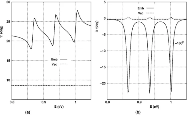
The ellipsometric angles⌿ and ⌬ are important because they represent the experimental values which can be mea-sured with the highest accuracy. They obey the definitions

rpp

rss = tan⌿e i_⌬

. 共33兲

The ellipsometric angles are relative quantities as is clear from the definition in the sense that they do not depend upon the absolute intensities of the reflected light. Yet, since the phase shift⌬, can be obtained separately and independently from the relative intensity variation as represented by⌿, the full response function can be recovered. In this case this would mean the full polarizability of the embedded dot, if we assume the dielectric constant of the medium to be a known FIG. 7. Absorbance A for angle of incidence␪i= 60°.共a兲 Ass,共b兲 App. Dashed curves, vacuum共no embedding兲. Solid curves, embedding

(10)

parameter. For the ellipsometric angle⌿ the vacuum results are systematically below the embedded results, as can be seen in Fig. 8. The value of ⌿=8.6° as an average for the vacuum situation, corresponds to a value of 44 for the ratio between Rss and Rpp as found in Fig.6. The variation of⌿ for the vacuum case is about 2.5% for the investigated re-gion. For the embedded case the situation is very different. The mean value of⌿ centers now around 22.5° in agreement with the fact that the embedded Rssand Rppare one order of magnitude closer to each other now. The absolute variations in⌿ upon embedding have increased by two orders of mag-nitude as compared to the vacuum case. The observed behav-ior for⌬ cannot be connected to the reflectance’s Rssand Rpp since in these quantities the phase information is lost. We see that the vacuum and embedded values are 180° out of phase, meaning that rss and rpp have different sign. Also here the absolute variation in⌬ has greatly improved, well over one order of magnitude, upon embedding, but not as large as for ⌿, where the improvement amounts a full two orders of magnitude. The variation in both ellipsometric angles is comfortably within range of an ellipsometer, the weak reflec-tance, the infrared frequency and the low temperature re-quired for proper measurement conditions being more of a problem.

IV. SUMMARY AND CONCLUSIONS

For a system of nano-objects 共here quantum dots兲 we have derived a hybrid discrete-continuum model to describe the optical response of a square lattice of these dots. It is possible to model the optical behavior of this lattice by means of discrete excess dipoles against a uniform

back-ground共including the space occupied by the nano-objects兲 of the embedding dielectric host medium. For InAs quantum dots with ⑀= 15.15 embedded in GaAs with ⑀m= 13.1 and modelled by means of dielectric ellipsoids the excess polar-izability of the dot can be larger than the normal polarizabil-ity of the same quantum dot in vacuum. All electromagnetic interactions in the system, either between the quantum dots or inside the quantum dot itself, turn out to be screened by the dielectric constant of the host material. This may seem obvious, but the internal electromagnetic interactions inside a free quantum dot are, in contrast, not screened. The dy-namical quantum mechanical contributions responsible for both the magnetic field and the frequency dependence are calculated in a Kramers-Heisenberg like fashion and added to the embedded bare polarizability. The first effect of the embedding upon the internal optical response is a decreased reflectance, but no more than a factor of 4. Most other as-pects of the response tend to increase upon embedding for the investigated quantum dot host combination. This holds for the structure in the reflectance, the absorbance and par-ticularly for the ellipsometric angles which have increased from measurable 共a few tenth of a degree兲 to large 共above 10 degree兲. Based upon this hybrid model and for this quan-tum dot host combination the influence of embedding is to increase the effects which can be used for applications.

ACKNOWLEDGMENT

This work is supported by the National Science Council of Taiwan under Contracts Nos. NSC-94-2811-M-009-020 and NSC-94-2112-M-009-037.

FIG. 8. Ellipsometric angles⌿, ⌬ for angle of incidence␪i= 60°.共a兲 ⌿共°兲, 共b兲 vacuum, ⌬共°兲; embedded, ⌬共°兲−180°. Dashed curves,

(11)

APPENDIX: DIELECTRIC OBLATE ELLIPSOID

Although a derivation of the electric fields for an oblate dielectric ellipsoid can be found in Stratton24 _{and more}

re-cently in Avelin,25_{the expressions given there are not suited}

for direct use. We will give a straightforward derivation here, using no implicit functions or unresolved integral expres-sions. Further we will keep the derivation as close as pos-sible to the derivation by Jackson17 _{for the spherical case}

enabling the shortcuts used in this paper. We consider the oblate ellipsoid with short axis c and long axis a as treated in Ref. 6 We will use again␨= c / a. For the transformation to elliptic coordinates we use

x = f cosh␰cos␩cos␾, y = f cosh␰cos␩sin␾,

z = f sinh␰sin␩, 共A1兲 where f =

冑

a2− c2. Because of the cylindrical symmetry of the problem共no␾dependence兲 we must solve the following Poisson equation for the electrostatic potential⌽共r兲:

冉

⳵2 ⳵␰2+ tanh␰ ⳵ ⳵␰+ ⳵2 d␩2− tan␩ ⳵ ⳵␩

冊

⌽ = 0. 共A2兲

This differential equation can be solved by separation of co-ordinates,

⌽共␩,␰兲 = G共␩兲F共␰兲. 共A3兲 A first solution to this differential equation is the externally applied uniform electric field E₀= E₀zˆ and its corresponding

potential⌽0:

⌽0共␩,␰,␾兲 = − E0z = G0共␩兲F0共␰兲, G0共␩兲 = − E0f sin␩,

F0共␰兲 = sinh␰. 共A4兲

Since the condition␰=␰₀establishes the surface of the oblate ellipsoid, varying␾,␩means scanning this surface. Freezing the␩ dependence to the one above, reduces the problem to one dimensional.

As a next ingredient to solve the dielectric ellipsoid, we need the solution F共␰兲 for a perfectly conducting sphere in a uniform electric field. For this case共A2兲 becomes

冉

⳵2

⳵␰2+ tanh␰

⳵

⳵␰− 2

冊

F共␰兲 = 0. 共A5兲

It is readily seen that F0共␰兲 is a solution as is easily verified by substitution. However we need one independent solution more, which can be shown to be

F1共␰兲 = 1 − sinh␰tan−1

冉

1

sinh␰

冊

. 共A6兲 We will use the functions F0共␰兲 and F1共␰兲 to solve the di-electric case.

The solution for the dielectric ellipsoid is based upon the superposition

⌽v共␰,␩,␾兲 = G0共␩兲关AvF0共␰兲 + BvF1共␰兲兴, 共A7兲 where the indexv equals I for the inner and O for the outer region of the ellipsoid, making four unknowns in total. Two of the unknowns can be eliminated by requiring that the electric field inside is constant and that the electric field out-side for large ␰ must coincide with the externally applied field E0. As a result BI= 0 and AO= 1. The remaining coeffi-cients AI, BOfollow from the boundary conditions:

We use AIto determine the electric field inside the ellipsoid,

EI= AIE0=

⑀m共h1− h2兲

⑀m共h1− h2兲 + 共⑀−⑀m兲h1

Eo 共A11兲

with which we can determine the polarizability ␣ and the excess polarizability␣X used in this paper共as ␣兲,

␣E₀= VP =⑀₀V␹EI=⑀0V⑀m

冉

⑀− 1 ⑀m+共⑀−⑀m兲Nz

冊

E₀, ␣XE0= V共P − Pm兲 =⑀0V共␹−␹m兲EI =⑀₀V

冉

⑀m共⑀−⑀m兲 ⑀m+ Nz共⑀−⑀m兲

冊

E₀, Nz= h1 h1− h2 , 共A12兲

where V =4₃␲a2_{c is the volume of the ellipsoid and the} sus-ceptibility ␹=⑀− 1. The depolarization factor Nz is exclu-sively determined by the values of the eigenfunctions of the problem at the boundary␰0 and accounts for the shape de-pendence. To make the expression more accessible we use that

(12)

sinh␰0= c

冑

a2− c2=

␨

冑

1 −␨2 共A13兲

and this enables us to write

h1=

冑

1 −␨2 ␨ − tan−1

冉

冑

1 −␨2 ␨

冊

, h₁− h₂=共1 −␨ 2_兲3/2 ␨ , 共A14兲

and we find for the depolarization factor Nz,

Nz= 1 1 −␨2

冉

1 −

␨cos−1␨

冑

1 −␨2

冊

共A15兲

which is exactly the same as the depolarization factor ob-tained by Avelin25 _{and for} _⑀

m= 1 this depolarization factor produces also Avelin’s polarizability when used in 共A12兲.

For the treatment of the embedded case when ⑀m⬎1 the reader is referred to the text.

The real benefit of this derivation is in the expressions for the external field EO共r兲,

EO共r兲 = E0− BO⵱ G0共␩兲F1共␰兲 = E0+ EE共r兲. 共A16兲 We refrain from the details and give only the final result in cylindrical coordinates,

EE共r兲 = E_␳␳ˆ + Ezzˆ,

r =␳␳ˆ + zzˆ =

冑

x2+ y2␳ˆ + zzˆ,

, 共A18兲

where the crucial auxiliary variable S is defined by S =

冑

s2+ z˜2_{− s,}

s =1₂关1 − 共˜␳2_{+ z}_˜2_兲兴, _共A19兲 where u˜ = u / f u =␳, z. Using these expressions for the outer field, backtransformation to cylindrical coordinates is estab-lished, but those coordinates are equivalent to Cartesian, be-cause of the cylindrical symmetry of the problem. Since the outer electric field expressions are explicit functions of the Cartesian coordinates, they are suited for direct use.

1_{V. G. Veselago, Sov. Phys. Usp. 10, 509}_共1968兲.

2_{J. B. Pendry et al., IEEE Trans. Microwave Theory Tech. 47,} 2075共1999兲.

3_{O. Voskoboynikov, G. Dyankov, and C. M. J. Wijers,} Microelec-tron. J. 36, 564共2005兲.

4_{R. A. Shelby, D. R. Smith, and S. Schulz, Science 292, 79} 共2001兲.

5_{C. M. J. Wijers, Phys. Rev. A 70, 063807}_共2004兲.

6_{O. Voskoboynikov, C. M. J. Wijers, J. L. Liu, and C. P. Lee, Phys.} Rev. B 71, 245332共2005兲.

7_{C. M. J. Wijers and P. L. de Boeij, J. Chem. Phys. 116, 328} 共2002兲.

8_{O. Stier, M. Grundmann, and D. Bimberg, Phys. Rev. B 59, 5688} 共1999兲.

9_{G. W. Bryant, Phys. Rev. B 37, 8763}_共1988兲.

10_{P. Enders, A. Bärwolff, M. Woerner, and D. Suisky, Phys. Rev. B}

51, 16695共1995兲.

11_{J. I. Climente, J. Planelles, and W. Jaskolski, Phys. Rev. B 68,} 075307共2003兲; J. Climente et al., J. Phys.: Condens. Matter 15, 3593共2003兲.

12_{C. G. Darwin, Proc. R. Soc. London, Ser. A 146, 17}_共1934兲.

13_{P. Noziéres and D. Pines, Phys. Rev. 109, 762}_共1958兲. 14_{O. Keller, J. Opt. Soc. Am. B 11, 1480}_共1994兲. 15_{S. L. Adler, Phys. Rev. 126, 413}_共1962兲. 16_{N. Wiser, Phys. Rev. 129, 62}_共1963兲.

17_{J. D. Jackson, Classical Electrodynamics} _{共Wiley, New York,} 1972兲.

18_{S. L. Chuang, Physics of Optoelectronic Devices} _{共Wiley, New} York, 1995兲.

19_{J. Vlieger, Physica}_{共Amsterdam兲 64, 63 共1973兲; C. M. J. Wijers} and K. M. E. Emmett, Phys. Scr. 38, 435共1988兲.

20_{O. Litzman and P. Rózsa, Surf. Sci. 66, 542}_共1977兲.

21_{G. P. M. Poppe, C. M. J. Wijers, and A. van Silfhout, Phys. Rev.} B 44, 7917共1991兲.

22_{C. M. J. Wijers and G. P. M. Poppe, Phys. Rev. B 46, 7605} 共1992兲.

23_{H. A. Kramers and W. Heisenberg, Z. Phys. 31, 681}_共1925兲. 24_{J. A. Stratton, Electromagnetic Theory}_{共McGraw-Hill, New York,}

1941兲.

25_{J. Avelin, Ph.D. thesis, Electromagnetics Laboratory, Helsinki} University of Technology, Report 414, 2003.