Energies 2012, 5, 545-560; doi:10.3390/en5030545
energies
ISSN 1996-1073 www.mdpi.com/journal/energies Article
Predicting High or Low Transfer Efficiency of Photovoltaic
Systems Using a Novel Hybrid Methodology Combining
Rough Set Theory, Data Envelopment Analysis and
Genetic Programming
Yi-Shian Lee 1,* and Lee-Ing Tong 2
1 Research Center for Psychological and Educational Testing, National Taiwan Normal University,
HePing East Rd., Section 1, Taipei 106, Taiwan
2 Department of Industrial Engineering Management, National Chiao Tung University,
1001 Ta-Hsuch Rd., Hsunchu 300, Taiwan; E-Mail: [email protected]
* Author to whom correspondence should be addressed; E-Mail: [email protected]; Tel.: +886-2-23683967 (ext. 15).
Received: 24 January 2012; in revised form: 13 February 2012 / Accepted: 20 February 2012 / Published: 27 February 2012
Abstract: Solar energy has become an important energy source in recent years as it generates less pollution than other energies. A photovoltaic (PV) system, which typically has many components, converts solar energy into electrical energy. With the development of advanced engineering technologies, the transfer efficiency of a PV system has been increased from low to high. The combination of components in a PV system influences its transfer efficiency. Therefore, when predicting the transfer efficiency of a PV system, one must consider the relationship among system components. This work accurately predicts whether transfer efficiency of a PV system is high or low using a novel hybrid model that combines rough set theory (RST), data envelopment analysis (DEA), and genetic programming (GP). Finally, real data-set are utilized to demonstrate the accuracy of the proposed method.
Keywords: photovoltaic systems; rough set theory; data envelopment analysis; genetic programming; hybrid model
Energies 2012, 5 546 1. Introduction
Although traditional energy resources, such as oil and coal, account for the largest proportion of energy worldwide, they also produce more pollution than solar energy. As environmental awareness and the need to reduce pollution have increased, solar energy has become an important energy source in industrialized countries. Photovoltaic systems convert solar energy into electrical energy. However PV systems are not yet popular and their transfer efficiency must be improved. Hence, engineers have used various combinations of system components to increase the transfer efficiency of PV systems. Generally, the transfer efficiency of a PV system is only 6–20% [1]. According to the options of experts in PV energy of Taiwan, a transfer efficiency exceeding 9% is considered high and that ≤9% is considered low [2]. Generally, engineers or energy managers must judge if a PV system belongs to one category or the other, thus, a reliable prediction model is needed to determine whether the transfer efficiency of a PV system is high or low. Managers or decision-makers in the PV field will then be able to identify the critical components using the prediction model and improve to transfer efficiencies. Thus, this work develops a novel and efficient prediction model to determine whether transfer efficiency of a PV system is high or low.
In applications of discriminating models, most studies utilized different approaches to construct an effective prediction model [3–7]. These models were constructed using conventional statistical methods, such as discriminant analysis and logistic regression, or artificial intelligence (AI) methods, such as artificial neural networks (ANNs) and support vector machines (SVMs). Ong et al. [8] demonstrated that a discriminating model constructed using an ANN-based method is more accurate than a model constructed using traditional statistical methods, especially when data-sets are non-linear. However, ANN-based discriminating models have poor prediction accuracy when applied to small samples and input variables are irrelevant [9]. Additionally, hidden layers in an ANN are difficult to explain and the relationship between input variables and output variables in an ANN or SVM cannot be expressed by a mathematical equation. Genetic programming (GP) has recently been applied in many fields to construct classification or prediction models. Since GP does not require any assumptions about the relationships between dependent and independent variables to construct a prediction model [10], GP can be applied to both small and large samples [8]. In some applications, GP has better prediction accuracy than ANN-based methods. For examples, Ong et al. [8] utilized GP to construct a more satisfactory credit scoring model than ANN model; Muttil and Lee [11] utilized GP to predict coastal algal blooms and claimed GP can obtain more effective prediction model than ANN in their analytical case. In prediction or classification applications, GP can be used to construct a mathematical equation [10–12]. Moreover, a comparison of the performance of classification models indicated that GP outperforms conventional statistical methods and ANNs [13].
Measuring and monitoring energy efficiency have become important issues in many fields [14]. Some studies have utilized data envelopment analysis (DEA) to assess energy efficiency. For instance, Boyd and Pang [15] examined the relationship between productivity and energy intensity utilizing DEA to assess productivity. Hu and Kao [16] developed an energy efficiency index utilizing DEA. This index is used to determine the energy-saving target ratio (ESTR) for seventeen APEC countries.
Energies 2012, 5 547 Based on the importance of energy efficiency and the ability of DEA to determine the ratio between input and output variables, this work adopts DEA to evaluate the input/output efficiency of PV systems using multiple inputs, such as texture type, selection of a PV module, and PV module capacity, and one output (transfer efficiency of PV systems).
Moreover, identifying significant input variables is important when constructing an effective prediction model. Many conventional methods, such as correlation analysis, have been utilized to identify the significant input variables for predicting the output variable. However, such methods are restricted by some assumptions, such as a linear relationship among variables and normality, and large data-sets. Thus, a technique that provides a knowledge system contained in a data-set and clear attribute selection under different classes is desirable. Rough set theory (RST) can be utilized as a soft computing tool to deal with data-sets with poor information and remove irrelevant attributes from a data-set [17]. Notably, RST has been applied in many real-world classification problems [18–20].
To construct an efficient prediction model that determines whether the transfer efficiency of a PV system is high or low, this work uses input/output efficiency of a PV system as the predictive variable and enhances prediction accuracy using a novel hybrid model combining RST with GP; this model is called the RST-GP model. Because of its robust reliability in knowledge systems, RST is utilized during the first stage to identify significant input variables. During the second stage, significant independent variables obtained from RST are utilized as input variables for GP to construct a prediction model that can determine whether the transfer efficiency of a PV system is high or low. This remainder of this paper is organized as follows. Section 2 reviews the PV system literature. Section 3 briefly reviews the DEA model used to evaluate the input/output efficiency of a PV system. Section 4 describes RST and GP. Section 5 elucidates the proposed hybrid model. Section 6 analyzes and compares the outcomes of the proposed and existing hybrid models. Section 7 gives conclusions. 2. An Overview of PV System
This section introduces the structure of PV system and factors influencing PV system transfer efficiency.
Energies 2012, 5 548 2.1. PV System
A PV system primarily consists of a solar cell, an electrical conditioner, an inverter, and a system controller. A PV system uses an inverter to transform light energy into electrical energy. Figure 1 shows the PV system process.
2.2. Factors Influencing PV Systems
Gregg et al. [22] noted that numerous complex factors influence the efficiency of PV systems. These factors can be classified as internal or external factors. Internal factors include PV system texture, the azimuthal angle, transformation of the PV inverter, and selection of direct current (DC) voltage and an inverter. Among the internal factors, PV system texture, the most important factor, influences PV system transfer efficiency. Single crystal and polycrystals are common in PV systems. The azimuthal angle of a PV system is that at which most light is received given the absence of obstacles; thus, azimuthal angle varies with PV system location. The PV inverter transforms light energy into electrical energy. Selection of DC voltage and the inverter both influence PV system transfer efficiency. However, in the real world, the transformation of light energy into electrical energy is affected by dynamic changes in sunshine. Accordingly, the optimal transfer efficiency of a PV inverter cannot be attained in practice.
The two major external factors are described as follows: first, the amount of solar radiation strongly influences PV system transfer efficiency. Thus, the degree of solar radiation must also be considered when determining PV system transfer efficiency. Second, the temperature of a PV system affects the amount of electrical energy converted from light energy. Thus, determining the optimal temperature in a real environment is a major goal for energy experts.
2.3. Evaluating PV System Transfer Efficiency
Transfer efficiency of a PV system is the percentage of energy converted from light energy. The transfer efficiency formula is:
Transfer efficiency (%) = mou 100%
in
P
P × (1)
where P is maximum output electrical energy, and mou P is input light energy. As transfer efficiency in increases, the amount of energy a PV system generates increases.
3. Using DEA to Determine Efficiencies
Notably, DEA is a linear programming (LP)-based technique for evaluating decision-making units (DMUs) and deals with many decision-making problems by converting multiple output and input variables into a single comprehensive performance measure [23]. DEA is an extensively utilized non-parametric data analysis technique. For instance, Hu and Kao [16] utilized DEA to construct an energy efficiency index. This index is used to determine the energy-saving target ratio (ESTR) for
Energies 2012, 5 549 seventeen Asia-Pacific Economic Cooperation (APEC) countries. Tsai et al. [23] applied DEA with other measures to assess the magnitude of performance differences between leading telecom carriers. Guo and Tanaka [24] utilized a fuzzy DEA model to solve an efficiency evaluation problem with given fuzzy input and output data. Wu et al. [25] used the DEA-neural network approach to evaluate branch efficiency for a large Canadian bank. Additional detailed descriptions of DEA can be found elsewhere [26–28].
DEA, developed by Charnes, Cooper, and Rhodes (CCR) [28], was based on Farrell’s (1957) pioneering study of efficiency measures (relative efficiency or productivity of a specific DMU) [29]. Suppose data for each DMU, j=1, 2,...,n, comprise q positive outputs, y , 1, 2,...,rj r= q, and p positive inputs, x , ij i=1, 2,...,p. Let ho (o=1, 2,...,n) be the DMU whose relative efficiency is to be maximized. The DEA model is displayed as LP as follows:
Maximize 1 1 q ro ro r o p io io i u y h v x = = ∑ = ∑ (2) Subject to 1 1 1 q r rj r p i ij i u y v x = = ∑ ≤ ∑ , 0 r i u v ≥ ; 1, 2,...,i= p; 1, 2,...,r= q
where ,uro v are the variable weights of given to the rth output and ith input of the oth DMU, io respectively. Furthermore, u and ro v are decision variables of LP modeling used to determine the io relative efficiency of DMUo. Obviously, the maximum value (efficiency score), h , cannot exceed 1. o If 1ho = , the DMUo is called the constant returns to scale (CRS) frontier [30]. There are two CCR models in practice. One minimizes input variables, and the other maximizes output variables. In this work, in order to obtain maximum energy efficiency, the maximized output variables of the CCR model are utilized to obtain the optimal value for the objective function, h . o
4. Rough Set Theory and Genetic Programming
This section reviews the basic concepts of RST and GP. 4.1. Basic Concepts of Rough Set Theory
Pawlak [31] developed RST as a data-mining approach in 1982. RST has proved effective for data-sets with poor information or ambiguity and it can be applied in many fields [32–34]. Walczak and Massart [35] provided a detailed description of RST.
An information system can be represented as S=(U, R, V, f), where U is the universe (a finite set of objects, U = {x1,x2,…,xn}), R is a finite set of attributes (features and variables), r
r R
V V
∈
= ∪ , where Vr is the domain of attribute r, and f U R: × → is an information function such that V f x r
( )
, ∈Vr for allEnergies 2012, 5 550 extracting decision rules. Let P⊆ and XR ⊆ , the lower approximation of X in S by P is denoted U as PX , and the upper approximation of X in S by P is denoted as PX and are derived as follows:
{ | ( ) } PX = ∈x U Ind R ⊂ X (3) { | / ( ) } PX= ∈x U U Ind R ∩ ≠X φ (4) where:
{
}
/ ( ) ( , )i j , ( , )i ( , ),j U Ind R = x x ∈ ⋅U U f x r = f x r ∀ ∈r R (5)From Equations (3),(4), the boundary can be represented as follows:
( )
pPN X =PX PX− (6)
Hence, reducts can be obtained utilizing approximation spaces. Given an information system
(
,)
S = U R , and then the reduct RED(P), the minimal set of attributes is P⊆ , such that R ( ) ( ) P R r U =r U where: 1 ( ( )) 1| ( ) | ( ) ( ) | | n n i i i i P card P X P X r U card U U = = ∑ ∑ = = (7)
where r Up( ) is the ratio of all P-correctly classified objects to all objects (U) in the system. Furthermore, core is common to all reducts. For instance, COR(P) is the core of P when
( )
( )
COR P = ∩RED P . Reduction is a feature subset selection process. The selected feature subset retains its explanation ability and has minimal redundancy [36]. Core analysis results can be represented as a reference of important attributes in a knowledge system. Several RST-based reduction and feature-selection algorithms have been developed. For instance, Wen et al. [37] applied RST and a grey model to analyze the factors influencing gas breakdown. Li et al. [38] developed a grey-based rough set approach to solve a supplier-selection problem. Thangavel and Pethalakshmi [39] reviewed studies using RST-based feature selection.
4.2. Genetic Programming
Koza [40] developed GP as a novel algorithm for computer programs that exploits evolution in solving model structure identification problems and performs symbolic regression [41]. The basic concepts of GP resemble those of genetic algorithms (GAs), and include mutation, crossover, and reproduction [10]. Unlike GAs, GP uses a generic parse-tree representation to replace the logic number of the genetic state (0 and 1). Additionally, GP can construct an optimal forecasting equation through symbolic regression. The main advantage of symbolic regression is that it is not limited to any functional form or normality assumption for data-sets. For instance, GP is more flexible in symbolic setting than conventional regression method or data-mining approach (e.g., ANN). Notably, GP is also widely utilized in practical applications such as in forecasting [10–12,42] and classification [8,43].
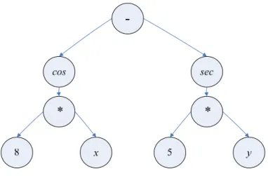
Functions or statements in GP have operators ({+, −, ×, ÷, log, and exp}) and a trigonometric function ({sin, cos, and tan}). Hence, a GP parse tree (Figure 2) can be applied to a simple example:
Energies 2012, 5 551 cos[8x] − sec[5y]. When selecting input variables, GP automatically finds variables that contribute most to the model [11,42] and does not have any restriction for data size, as compared to an ANN or large data-set [8,43].
Figure 2. Example of GP parse tree representation.
5. The Proposed Hybrid Prediction Model
This work develops a four-step procedure for predicting whether the transfer efficiency of a PV system is high or low. The proposed prediction model is as follows:
Step 1: Collect transfer efficiencies of PV systems with various component combinations. These components are independent variables and transfer efficiency is a binary output variable (i.e., high or low) in the proposed prediction model.
Step 2: RST selects the significant independent variables of a PV system based on its robust reliability in knowledge system [36–39]. The importance of feature selection based on RST (i.e., core analysis) can be explained as follows [44]:
( )
( )
( )
{ }( )
( )
{ }( )
( )
, 1 C C a C a C D C C D D D a D D γ γ γ σ γ γ − − − = = − (8)where γC
( )
D denotes the degree of dependence between conditional features C (the variables of PVsystems) and decision feature D (i.e., the high or low PV transfer efficiency), γC−{ }a
( )
D denotes thedegree of dependence between removing a conditional feature (such as a condition feature) from C and decision feature D. σ(C D, )
( )
a denotes the variation of degree of dependence between removing a from C with all condition features C. When σ(C D, )( )
a is large, feature a importantly affects the decision attribute D.Step 3: The DEA evaluates energy efficiency (i.e., the input/output ratio) of a PV system. The input variables in DEA are obtained in Step 2 and the output variable in DEA is transfer efficiency of a PV system. The DMU values obtained from DEA represent energy efficiencies of PV systems.
Step 4: GP constructs a classification model for predicting whether transfer efficiency of a PV system is high or low. For the GP model, this work utilizes the significant independent variables obtained in Step 2 and the input/output ratio obtained in Step 3 as input variables of GP and binary
Energies 2012, 5 552 transfer efficiency (i.e., high or low) of a PV system is the output variable of GP. Table 1 presents parameter settings of the GP model. The parameters of GP are obtained by trial-and-error approach.
Table 1. The settings of GP model.
Items Content
Population size 400
Maximum number of generation 1000
Function set +, −, ×, ÷, sin, cos, exp, log constant
Crossover rate 0.8
Mutation rate 0.02
In Step 2, RST is utilized to select the significant independent variables of PV systems because adopting significant independent variables can yield good accuracy for constructing a prediction model [36]. Moreover, RST can not only deal with small data-sets but also requires no statistical assumptions (such as a linear relationship between input variables with output variable). In Step 3, DEA is utilized to evaluate the energy efficiency of PV systems because the index (energy efficiency of PV systems) efficiently provides sufficient information for evaluating the economic-value of PV systems. In Step 4, GP is utilized to construct a prediction model because of its high performance in forecasting and classification. Furthermore, GP yields good forecasts using only small data-sets [42]. Hence, RST, DEA, and GP are integrated herein to predict the high or low transfer efficiency of PV systems, and the model thus developed is called the RST-DEA-GP model.
6. Empirical Analysis
A real data-set of transfer efficiency of PV systems collected from a Taiwanese research organization is utilized to demonstrate the effectiveness of the proposed model. The data used in Step 1 concern 38 PV systems. Each PV system contains 18 variables (e.g., texture type, capacity for PV-transfer, and number of inverters) and binary transfer efficiency (e.g., low or high). The low and high transfer efficiencies of the PV systems are coded as 0 and 1, respectively. The data-set comprises 38 PV systems–15 with low and 23 with high transfer efficiencies.
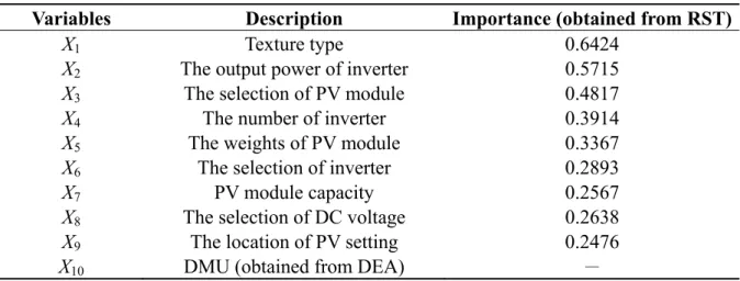
Table 2. Selected significant variables from RST and DMU variable from DEA. Variables Description Importance (obtained from RST)
X1 Texture type 0.6424
X2 The output power of inverter 0.5715
X3 The selection of PV module 0.4817
X4 The number of inverter 0.3914
X5 The weights of PV module 0.3367
X6 The selection of inverter 0.2893
X7 PV module capacity 0.2567
X8 The selection of DC voltage 0.2638
X9 The location of PV setting 0.2476
Energies 2012, 5 553 In Step 2 of the proposed hybrid model, RST is utilized to identify significant independent variables of PV systems. The RST algorithm can be constructed using MATLAB software. The RST results indicate that nine independent variables (X1–X9) are significant (Table 2) because that the importance
value of nine independent variables are greater than 0.2. It has not a clear criterion to determine the threshold value (importance value). Moreover, the nine independent variables (X1–X9) have high
correlation to output variable (the low or high transfer efficiencies of PV systems). The correlation coefficient are greater than 0.6. Also, based on the opinion of experts in PV energy in Taiwan, these nine variables importantly influence for the transfer efficiency of PV systems.
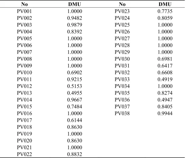
In Step 3, DEA is utilized to evaluate the DMU value of each PV system. Table 2 shows the DMU value (X10). In applying DEA, input variables of DEA are the nine significant variables obtained in
Step 2 and the output variable of DEA is PV system transfer efficiency. The DEA algorithm can be executed by LINGO software. Table 3 lists the DMU values of the PV systems. In Step 4, the significant independent variables obtained in Step 2 and DMU obtained in Step 3 are utilized as input variables for GP to predict the high or low level of PV system transfer efficiency. To demonstrate the effectiveness of the proposed hybrid model, some basic classification models such as K Nearest Neighbor (KNN), Naive Bayes (NB), SVM, ANN, and GP are utilized as benchmark models. The basic classification models belong to data-mining techniques and can obtain better prediction performance than traditional linear statistical method (e.g., linear regression) [8,10].
Table 3. The results of DMU value of each PV system by utilizing DEA.
No DMU No DMU PV001 1.0000 PV023 0.7735 PV002 0.9482 PV024 0.8059 PV003 0.9879 PV025 1.0000 PV004 0.8392 PV026 1.0000 PV005 1.0000 PV027 1.0000 PV006 1.0000 PV028 1.0000 PV007 1.0000 PV029 1.0000 PV008 1.0000 PV030 0.6981 PV009 1.0000 PV031 0.6417 PV010 0.6902 PV032 0.6608 PV011 0.9215 PV033 0.4919 PV012 0.5153 PV034 1.0000 PV013 0.4955 PV035 0.8274 PV014 0.9667 PV036 0.4947 PV015 0.7484 PV037 0.8405 PV016 1.0000 PV038 0.9944 PV017 0.6144 PV018 0.8630 PV019 1.0000 PV020 0.8630 PV021 1.0000 PV022 0.8832
Energies 2012, 5 554 Although some studies [36] have also adopted hybrid classification models that combine RST, DEA, and SVM to predict business failures, the RST of their proposed methodology did not identify how to obtain the important variables based on a clear equation. This study [36] only adopted the RSES software tool [45] to select important variables. Furthermore, the SVM model performs well only with large data-sets, and collecting large data-sets for PV systems is difficult. Hence, the use of a suitable classification model for small data-sets is important for constructing a high-precision prediction model. In order to compare the accuracy of hybrid prediction model when adding DEA or nor, this work does some design of experiments for prediction models. The proposed model, named RST-DEA-GP model, which adopts the significant variables obtained by RST and the DMU variable obtained in DEA as input variables for GP (model I). The RST-GP model adopts only the significant variables, X1–X9, as
the input variables for GP (model II). In both models I and II, this work adopts leave-one-out cross validation to test the accuracy of the prediction model.
Tables 4 and 5 show the analytical results for hybrid models I and II, respectively. Model I has an average correct classification rate of 92.10%, and that of model II is 84.21%. Hence, adding DEA provides more information than adopting significant input variables only and enhances prediction model accuracy.
Table 4. RST-DEA-GP model (model I) results with both significant variables and DMU.
Actual class Classified class
1 (High-level) 2 (Low-level)
1 (High-Level) 22 (95.65%) 1 (4.35%)
2 (Low-Level) 2 (13.33%) 13 (86.67%)
Average correct classification rate: 92.10%.
Table 5. RST-GP model (model II) results with only significant variables.
Actual class Classified class
1 (High-level) 2 (Low-level) 1 (High-Level) 21 (91.30%) 2 (8.70%)
2 (Low-Level) 4 (26.67%) 11 (73.33%)
Average correct classification rate: 84.21%.
The RST-SVM-based models are also utilized to predict whether PV systems have high or low transfer efficiency. The RST-DEA-SVM model uses both significant variables obtained from RST and DMU as input variables of SVM (model III). The RST-SVM model, which utilizes only significant attributes, is model IV. In constructing the SVM model, this work utilizes STATISTICA software to generate a classification model. Some studies [46,47] utilized the Gaussian kernel function to enhance prediction performance. For the SVM model, parameters settings are the Gaussian kernel function, C = 3, and r =0.129, which can generate an appropriate prediction model. Tables 6 and 7 summarize prediction results for the confusion matrix utilizing models III and IV, respectively. Based on RST-SVM-based model results, adding DEA improves the correct classification rate from 78.94% to 81.57%.
Energies 2012, 5 555 Table 6. RST-DEA-SVM model (model III) results with significant variables and DMU.
Actual class Classified class
1 (High-level) 2 (Low-level) 1 (High-Level) 20 (86.96%) 3 (13.04%)
2 (Low-Level) 4 (26.67%) 11 (73.33%)
Average correct classification rate: 81.57%.
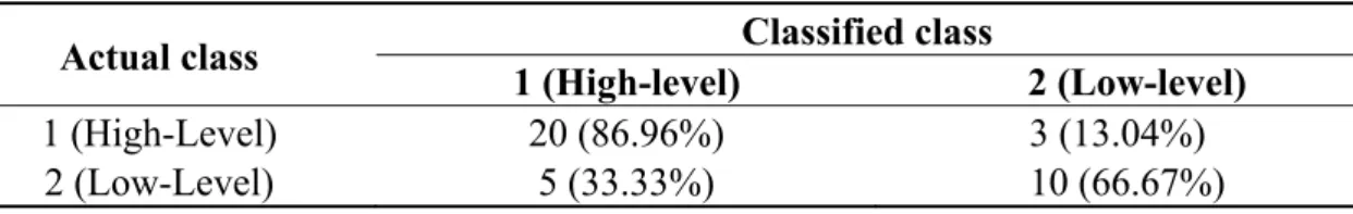
Table 7. RST-SVM model (model IV) results with only significant variables.
Actual class Classified class
1 (High-level) 2 (Low-level) 1 (High-Level) 20 (86.96%) 3 (13.04%)
2 (Low-Level) 5 (33.33%) 10 (66.67%)
Average correct classification rate: 78.94%.
Furthermore, two RST-ANN-based prediction models are applied. One uses the significant variables obtained from RST and the DMU variable obtained from DEA as input variables for an ANN (model V, named RST-DEA-ANN model). The RST-ANN model utilizes only significant variables as input variables for the ANN (model VI). This work uses Qnet2000 software to construct the ANN classification model. Cybenko [48] demonstrated that utilizing one hidden layer is sufficient when modeling any complex system. Hence, the appropriate network models are 10-5-1 and 9-7-1 for nodes of the input layer, hidden layer, and output layer for models V and VI, respectively. Tables 8 and 9 summarize prediction results for the confusion matrix utilizing models V and VI, respectively. Similarly, from the results of RST-SVM-based model, RST-ANN is also obvious that adding DEA can improve the correct classification rate from 76.31% to 81.57%.
Table 8. RST-DEA-ANN model (model V) results with both significant variables and DMU.
Actual class Classified class
1 (High-level) 2 (Low-level) 1 (High-Level) 21 (91.30%) 2 (8.70%)
2 (Low-Level) 5 (33.37%) 10 (66.67%)
Average correct classification rate: 81.57%.
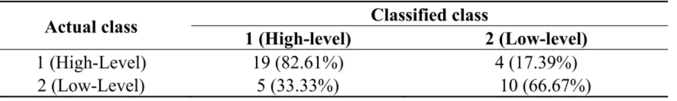
Table 9. RST-ANN model (model VI) results with only significant variables.
Actual class Classified class
1 (High-level) 2 (Low-level) 1 (High-Level) 19 (82.61%) 4 (17.39%)
2 (Low-Level) 5 (33.33%) 10 (66.67%)
Average correct classification rate: 76.31%.
With the same analysis of the above classification models (model I to VI), two RST-KNN-based and RST-NB-based prediction models are applied to predict whether PV systems have high or low transfer efficiency. This work also adopts STATISTICA to construct the KNN and NB classification
Energies 2012, 5 556 models, respectively. For KNN classification, one uses the significant variables obtained from RST and the DMU variable obtained from DEA as input variables for a KNN (model VII, named RST-DEA-KNN model). The RST-KNN model utilizes only significant variables as input variables for the KNN (model VIII). Tables 10 and 11 summarize prediction results for the confusion matrix utilizing models VII and VIII, respectively. Based on RST-KNN-based model results, adding DEA improves the correct classification rate from 73.68 % to 76.31%.
Table 10. RST-DEA-KNN model (model VII) results with both significant variables and DMU.
Actual class Classified class
1 (High-level) 2 (Low-level) 1 (High-Level) 19 (82.61%) 4 (17.39%)
2 (Low-Level) 5 (33.33%) 10 (66.67%)
Average correct classification rate: 76.31%.
Table 11. RST-KNN model (model VIII) results with only significant variables.
Actual class Classified class
1 (High-level) 2 (Low-level)
1 (High-Level) 18 (78.26%) 5 (21.74%)
2 (Low-Level) 5 (33.33%) 10 (66.67%)
Average correct classification rate: 73.68%.
For NB classification, one uses the significant variables obtained from RST and the DMU variable obtained from DEA as input variables for a NB (model IX, named RST-DEA-NB model). The RST-NB model utilizes only significant variables as input variables for the NB (model X). Tables 12 and 13 summarize prediction results for the confusion matrix utilizing models IX and X, respectively. Based on RST-NB-based model results, adding DEA improves the correct classification rate from 73.68 % to 76.31%.
Table 12. RST-DEA-NB model (model IX) results with both significant variables and DMU.
Actual class Classified class
1 (High-level) 2 (Low-level) 1 (High-Level) 19 (82.61%) 4 (17.39%)
2 (Low-Level) 5 (33.33%) 10 (66.67%)
Average correct classification rate: 76.31%.
Table 13. RST-NB model (model X) results with only significant variables.
Actual class Classified class
1 (High-level) 2 (Low-level) 1 (High-Level) 19 (82.61%) 4 (17.39%)
2 (Low-Level) 6 (40%) 9 (60%)
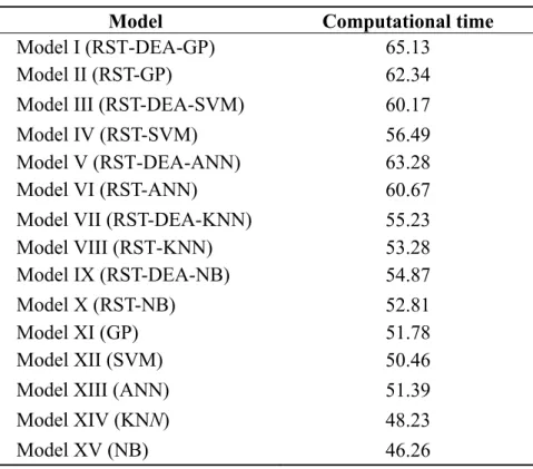
Energies 2012, 5 557 To compare the performance of models I to XII with that of basic classification models (GP, SVM, ANN, KNN, and NB models), the latter, basic classification models are utilized to construct the prediction model. Additionally, the original 18 variables of the PV system are taken into account as the input variables of each basic classification model and the output variable is the binary transfer efficiency (high or low) of a PV system. The results (average correct classification rate) of the basic classification models, based on leave-one-out cross validation are: GP (84.21%, model XI), SVM (78.94%, model XII), ANN (78.94%, model XIII), KNN (71.05%, model XIV), and NB (68.42%, model XV). To determine the computational demands of all classification models (model I to XV), the computing time of each is calculated (Table 14).
Table 14. Computational time of different models (seconds).
Model Computational time
Model I (RST-DEA-GP) 65.13
Model II (RST-GP) 62.34
Model III (RST-DEA-SVM) 60.17 Model IV (RST-SVM) 56.49 Model V (RST-DEA-ANN) 63.28
Model VI (RST-ANN) 60.67
Model VII (RST-DEA-KNN) 55.23 Model VIII (RST-KNN) 53.28 Model IX (RST-DEA-NB) 54.87
Model X (RST-NB) 52.81
Model XI (GP) 51.78
Model XII (SVM) 50.46
Model XIII (ANN) 51.39
Model XIV (KNN) 48.23
Model XV (NB) 46.26
These analytical results demonstrate that the proposed hybrid model is more accurate than other hybrid models in predicting whether the transfer efficiency of PV systems is high or low. Although the computational time of the proposed model exceeds that of the other models, its prediction of whether the transfer efficiency of PV systems is low or high is very precise. Notably, adding the DMU variable, obtained from DEA, as an independent variable to the GP, SVM, ANN, KNN and NB models yields more information than considering only significant variables, and enhances the classification accuracy rate of the proposed model. Finally, the proposed model can obtain greater performance than only adopting one classification model (GP).
7. Conclusions
Accurately predicting high or low transfer efficiency of a PV system is difficult since many uncertain factors may influence correct classifications of real-world data. This work makes four
Energies 2012, 5 558 important contributions to the existing literature. First, adding DEA provides additional information for constructing a model that can predict high or low transfer efficiency of PV systems. Second, the results of RST can allow managers or decision-makers in the PV field to identify the critical components. Third, the proposed hybrid model has better classification results than existing hybrid models, regardless of whether only significant variables are adopted or significant variables and the DMU variable are adopted. Fourth, the proposed model also has the lowest misclassification rate among all models tested. Therefore, the proposed RST-DEA-GP model can accurately predict whether a PV system has high or low transfer efficiency.
Future work can apply grey theory to determine whether a PV system has high or low transfer efficiency based on uncertain information. Second, in order to demonstrate the effectiveness of the proposed hybrid prediction model, it will be utilized to predict more different country PV systems. References
1. Bureau of Energy, Ministry of Economic. Available online: http://www.moeaboe.gov.tw (accessed on 13 February 2012).
2. Industrial Technology Research Institute. Available online: http://www.solar.org.tw/aboutus/sense/ battery.asp (accessed on 13 February 2012).
3. Zhou, X.; Liu, K.Y.; Wong, S.T.C. Cancer classification and prediction using logistic regression with Bayesian gene selection. J. Biomed. Inf. 2004, 37, 249–259.
4. Worth, A.P.; Cronin, M.T.D. The use of discriminant analysis, logistic regression and classification tree analysis in the development of classification models for human health effects. J. Mol. Struct. Theochem. 2003, 622, 97–111.
5. Kurt, I.; Ture, M.; Kurum, A.T. Comparing performances of logistic regression, classification and regression tree, and neural networks for predicting coronary artery disease. Expert Syst. Appl. 2008, 34, 366–374.
6. Huang, Z.; Chen, H.; Hsu, C.J.; Chen, W.H.; Wu, S. Credit rating analysis with support vector machines and neural networks: a market comparative study. Decis. Support Syst. 2004, 37, 543–558. 7. Luts, J.; Ojeda, F.; Plas, R.V.D.; Moor, B.D.; Huffel, S.V.; Suykens, J.A.K. A tutorial on support
vector machine-based methods for classification problems in chemometrics. Anal. Chim. Acta 2010, 665, 129–145.
8. Ong, C.S.; Huang, J.J.; Tzeng, G.H. Building credit scoring models using genetic programming. Expert Syst. Appl. 2005, 29, 41–47.
9. Nath, R.; Rajagopalan, B.; Ryker, R. Determining the saliency of input neural classifiers. Comput. Oper. Res. 1997, 24, 767–773.
10. Lee, D.G.; Lee, B.W.; Chang, S.H. Genetic programming model for long-term forecasting of electric power demand. Electr. Power Syst. Res. 1997, 40, 17–22.
11. Muttil, N.; Lee, J.H.W. Genetic programming for analysis and real-time prediction of coastal algal blooms. Ecol. Model. 2005, 189, 363–376.
Energies 2012, 5 559 12. Liong, S.Y.; Gautam, T.R.; Khu, S.T.; Babovic, V.; Muttil, N. Genetic Programming: a new
paradigm in rainfall-runoff modelling. J. Am. Water Res. Assoc. 2002, 38, 557–584.
13. Zhang, Y.; Bhattacharyya, S. Genetic Programming in classifying large-scale data: an ensemble method. Inf. Sci. 2004, 163, 85–101.
14. Ang, B.W. Monitoring changes in economy-wide energy efficiency: From energy-GDP ratio to composite efficiency index. Energy Policy 2006, 34, 574–582.
15. Boyd, J.X.; Pang, T.G. Estimating the linkage between energy efficiency and productivity. Energy Policy 2000, 28, 289–296.
16. Hu, J.L., Kao, C.H. Efficiency energy-saving targets for APEC economies. Energy Policy 2007, 35, 373–382.
17. Pawlak, Z. Rough sets and intelligent data analysis. Inf. Sci. 2002, 147, 1–12.
18. Ahn, B.S.; Cho, S.S.; Kim, C.Y. The integrated methodology of rough set theory and artificial neural network for business failure prediction. Expert Syst. Appl. 2000, 18, 65–74.
19. Leung, Y.; Fischer, M.M.; Wu, W.Z.; Mi, J.S. A rough set approach for the discovery of classification rules in interval-valued information systems. Int. J. Approx. Reason. 2008, 47, 233–246.
20. Dembczynski, K.; Greco, S.; Slowinski, R. Rough set approach to multiple criteria classification with imprecise evaluations and assignments. Eur. J. Oper. Res. 2009, 198, 626–636.
21. A Guide to Photovoltaic (PV) System Design and Installation. Available online: http://www.energy.ca.gov/reports/2001-09-04_500-01-020.PDF (accessed on 13 February 2012). 22. Gregg, A.; Parker, T.; Swenson, R. A “real world” examination of PV system design and
performance. In Proceeding of the IEEE Photovoltaic Specialists Conference, Austin, TX, USA, June 2005; pp. 1587–1592.
23. Tsai, H.C.; Chen, C.M.; Tzeng, G.H. The comparative productivity efficiency for global telecoms. Int. J. Prod. Econ. 2006, 103, 509–526.
24. Guo, P.; Tanaka, H. Fuzzy DEA: a perceptual evaluation method. Fuzzy Sets Syst. 2001, 119, 149–160.
25. Wu, D.; Yang, Z.; Liang, L. Using DEA-neural network approach to evaluate branch efficiency of a large Canadian bank. Expert Syst. Appl. 2006, 31, 108–115.
26. Banker, R.D.; Charnes, A.; Cooper, W.W. Some models for estimating technical and scale inefficiencies in data envelopment analysis. Manag. Sci. 1984, 30, 1078–1092.
27. Data Envelopment Analysis: Theory, Methodology and Applications; Charnes, A., Cooper, W.W., Lewin, A.Y., Seiford, L.M., Eds.; Springer: Boston, MA, USA, 1995.
28. Charnes, A.; Cooper, W.W.; Rhodes. E. Measuring the efficiency of decision making units. Eur. J. Oper. Res. 1978, 2, 429–444.
29. Farrell, M.J. The measurement of productive efficiency. J. R. Stat. Soc. Ser. A. Gen. 1957, 120, 253–289.
30. Chen, Y.; Ali, A.I. Output-input ratio analysis and DEA frontier. Eur. J. Oper. Res. 2002, 142, 476–479.
Energies 2012, 5 560 32. Shyng, J.Y.; Wang, F.K.; Tzeng, G.H.; Wu, K.S. Rough set theory in analyzing the attributes of
combination values for the Insurance Market. Expert Syst. Appl. 2007, 32, 56–64.
33. Swiniarski, R.W.; Skowron, A. Rough set methods in feature selection and recognition. Pattern Recogn. Lett. 2003, 24, 833–849.
34. Zhai, L.Y.; Khoo, L.P.; Fok, S.C. Feature extraction using rough set theory and genetic algorithms an application for the simplification of product quality evaluation. Comput. Ind. Eng. 2002, 43, 661–676.
35. Walczak, B.; Massart, D.L. Tutorial rough sets theory. Chemom. Intell. Lab. Syst. 1999, 47, 1–16. 36. Yeh, C.C.; Chi, D.J.; Hsu, M.F. A hybrid approach of DEA, rough set and support vector
machines for business failure prediction. Expert Syst. Appl. 2010, 37, 1535–1541.
37. Wen, K.L.; Wang, C.W.; Yeh, C.K. Apply rough set and GM (h,N) model to analyze the influence factor in gas breakdown. In Proceeding of IEEE International Conference on Systems, Man, and Cybernetics Society, London, UK, April 2007; pp. 2771–2775.
38. Li, G.D.; Yamaguchi, D.; Nagai, M. A grey-based rough decision-making approach to supplier selection. Int. J. Adv. Manuf. Technol. 2008, 1032–1040.
39. Thangavel, K.; Pethalakshmi, A. Dimensionality reduction based on rough set theory: A review. Appl. Soft Comput. 2009, 9, 1–12.
40. Koza, J. Genetic Programming: On the Programming of Computers by Natural Selection; MIT Press: Cambridge, MA, USA, 1992.
41. Davidson, J.W.; Savic, D.A.; Walters, G.A. Symbolic and numerical regression: Experiments and applications. Inf. Sci. 2003, 150, 95–117.
42. Lee, Y.S.; Tong, L.I. Forecasting energy consumption using a grey model improved by incorporating genetic programming. Energy Convers. Manag. 2011, 52, 147–152.
43. Huang, J.J.; Tzeng, G.H.; Ong, C.S. Two-stage genetic programming (2SGP) for the credit scoring model. Appl. Math. Comput. 2006, 174, 1039–1053.
44. Wen, K.L.; Nagai, M.; Chang, T.C.; Wen, H.C. An Introduction to Rough Set Theory and Application; Wu-Nan Book Co. Ltd.: Taipei, Taiwan, 2008.
45. Komorowski, K.; Ohrn, A.; Skowron, A. The ROSETTA rough set software system. In Handbook of Data Mining and Knowledge Discovery; Klosgen, W., Zytkow, J., Eds.; Oxford University Press: New York, NY, USA, 2002.
46. Pai, P.F.; Lin, C.S. A hybrid ARIMA and support vector machines model in stock price forecasting. Omega 2005, 33, 497–505.
47. Chen, K.Y.; Wang, C.H. A hybrid SARIMA and support vector machines in forecasting the production values of the machinery industry in Taiwan. Expert Syst. Appl. 2007, 32, 254–264. 48. Cybenko, G. Approximation by superpositions of a sigmoidal function. Math. Control Signal. Syst.
1989, 2, 303–314.
© 2012 by the authors; licensee MDPI, Basel, Switzerland. This article is an open access article distributed under the terms and conditions of the Creative Commons Attribution license (http://creativecommons.org/licenses/by/3.0/).
![Figure 1. A diagram of a PV system [21].](https://thumb-ap.123doks.com/thumbv2/9libinfo/7771037.150176/3.892.114.792.906.1101/figure-a-diagram-of-a-pv-system.webp)