This work was supported by National Science Council, Taiwan, under Grant no. NSC 99-2221-E-009-159. DOI: 10.3837/tiis.2011.12.006
Real-Time Vehicle Detector with Dynamic
Segmentation and Rule-based Tracking
Reasoning for Complex Traffic Conditions
Bing-Fei Wu and Jhy-Hong Juang
Department of Electrical Engineering, National Chiao Tung University 1001 Ta-Hsueh Road, Hsinchu 30050, Taiwan
[e-mail: [email protected]] *Corresponding author: Bing-Fei Wu
Received July 12, 2011; revised October 8, 2011; accepted November 23, 2011; published December 31, 2011
Abstract
Vision-based vehicle detector systems are becoming increasingly important in ITS applications. Real-time operation, robustness, precision, accurate estimation of traffic parameters, and ease of setup are important features to be considered in developing such systems. Further, accurate vehicle detection is difficult in varied complex traffic environments. These environments include changes in weather as well as challenging traffic conditions, such as shadow effects and jams. To meet real-time requirements, the proposed system first applies a color background to extract moving objects, which are then tracked by considering their relative distances and directions. To achieve robustness and precision, the color background is regularly updated by the proposed algorithm to overcome luminance variations. This paper also proposes a scheme of feedback compensation to resolve background convergence errors, which occur when vehicles temporarily park on the roadside while the background image is being converged. Next, vehicle occlusion is resolved using the proposed prior split approach and through reasoning for rule-based tracking. This approach can automatically detect straight lanes. Following this step, trajectories are applied to derive traffic parameters; finally, to facilitate easy setup, we propose a means to automate the setting of the system parameters. Experimental results show that the system can operate well under various complex traffic conditions in real time.
Keywords: Detection, segmentation, tracking, occlusion, rule-based reasoning, lane detection, prior occlusion resolution, traffic parameter
1. Introduction
A
multiple-vehicle detection and tracking (MVDT) system has the following applications: determining traffic parameters, detecting violations of traffic rules, detecting car accidents, classifying vehicles, and tracking vehicles. The advantages of MVDT are easy setup, low cost, a high degree of precision, and robustness. However, the efficiency of such a system is greatly affected by various complex traffic environments. Hence, most systems incorporate their own approaches for detection in order to overcome the effects of such complex traffic conditions. Unfortunately, an extra detection approach leads to greater computing effort, and hence, meeting real-time requirements becomes more challenging.Wang [1] proposed a joint random field (JRF) model for the detection of moving vehicles in video sequences. This method could take into account moving shadows, lights, and various weather conditions. However, the method could not perform vehicle classification or detect vehicle velocity. Tsai et al. [2] presented a novel vehicle detection approach for detecting vehicles from static images on the basis of color and edges. This approach involved a new color transform model to find important “vehicle color” information in order to quickly locate possible vehicle candidates. This approach could also be used for detecting vehicles in various weather conditions, but it does not address the resolution of vehicle occlusions. Zhang et al. [3]
developed a multilevel framework to detect and handle vehicle occlusion. The proposed framework consisted of an intra-frame, an inter-frame, and tracking levels to resolve vehicle occlusion. Neeraj et al. [4] presented a method for segmenting and tracking vehicles on highways using a camera that was positioned relatively closer to the ground. Melo [5]
proposed a low-level object tracking system that generated accurate vehicle motion trajectories, which could be further analyzed to detect lane centers and classify lane types. A lane-detection method aimed at handling moving vehicles in various traffic scenarios was proposed by Cheng et al. [6]. A new background subtraction algorithm based on the sigma-delta filter, which was intended to be used in urban traffic situations, was presented in
[7]. An example-based algorithm for moving vehicle detection was introduced in [8].
A double-difference operator (three-frame difference) [9] was used to detect vehicles from the magnitude of the gradient. This approach was more complicated than the previous scheme generally used, and also gathered more vehicle information. However, with this approach, it was difficult to overcome luminance changes caused by daylight, weather conditions, and the operation of automatic electric shutters (AES). Consequently, optical-flow-based techniques that estimated the intensity of motion between two subsequent frames were developed
[10][11]. These approaches required substantial computing time to obtain optimal solutions, even when some algorithms to enhance computing speed were applied. Segmentation methods
[12][13][14] that extracted a reference background to detect moving objects were better options for real-time applications. However, these methods were highly dependent on an initial background that had no disturbances from moving objects.
In this paper, a real-time MVDT system is developed to reduce the processing time, extract moving objects, and track vehicles in various complex traffic conditions. First, the background image is extracted by applying a segmentation algorithm [15] from a color image sequence. The current background image is regularly updated by referring to previous background images in order to ensure a more robust background extraction in circumstances where the degree of luminance is constantly changing. Moreover, this paper proposes a feedback procedure to resolve partial background updating errors, which occur in cases where vehicles
are temporarily parked on the roadside while the background image converges. In the tracking process, the relative distances and directions of moving objects are utilized to determine whether to create, extend, or delete tracking trajectories. There are two approaches for solving issues of vehicle occlusions. If the occlusion is detected in the early stages, rule-based tracking through reasoning is applied. If early detection fails, a lane mask that is obtained through the lane detection technique [16] based on the extracted background is used to distinguish occluded vehicles. Finally, traffic parameters are calculated from the tracking trajectories by referring to the lane mask. Moreover, to enable an easy setup, the automatic evaluation of traffic parameters is proposed. The work is organized as follows. Chapter 2 presents an overview of the system. Chapter 3 introduces the methods used in the process of dynamic segmentation, including extraction of the background, segmentation of moving objects, adaptation to illumination change, and compensation of the background. Chapter 4 explains automatic lane detection and the procedure of prior split by lane mask. Vehicle tracking and a strategy to update traffic parameters are proposed in Chapter 5. Chapter 6 addresses the experimental results obtained by the proposed system, and Chapter 7 presents the conclusions drawn from these results.
2. System Overview
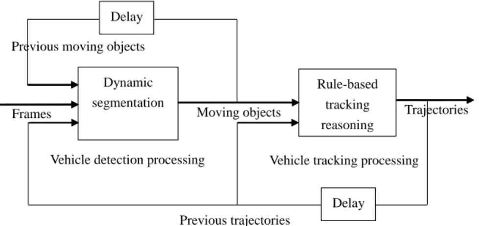
There are two important processes in the proposed MVDT system. One is dynamic segmentation, and the other is rule-based tracking through reasoning. In the first procedure, moving objects are segmented from video frames by referring to a regularly updated background as well as to previous tracking trajectories. There are several steps involved in the process of dynamic segmentation. First, the reference color background image is extracted. Second, moving objects are segmented by referring to the extracted background. Next, the background is modified to compensate for the changes in illumination. Finally, compensation for the background is applied and the automatic detection of straight lanes is performed. In the second procedure, the spatiotemporal characteristics of the moving objects are utilized to update their trajectories. The main goal here is to track the vehicles and calculate useful traffic parameters. The steps in this part include prior split by lane mask, filtration of falsely detected noises, updating of tracking trajectories, resolution of vehicle occlusions, and updating vehicle parameters. Fig. 1 shows the block diagram of the proposed MVDT system.
Vehicle detection processing Vehicle tracking processing Dynamic segmentation Rule-based tracking reasoning Delay Delay Previous trajectories Frames
Previous moving objects
Moving objects Trajectories
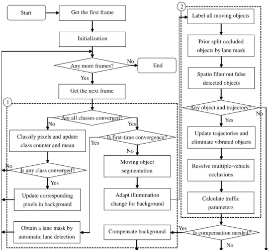
Fig. 2 presents a detailed flowchart of the MVDT system. The dashed-line regions 1 and 2 represent the sub-flowcharts for the procedures of dynamic segmentation and rule-based tracking through reasoning, respectively.
No
No
No
Are all classes converged?
Classify pixels and update class counter and mean
Yes
Update corresponding pixels in background
Moving object segmentation Is any class converged?
Yes
Any more frames? Initialization Get the first frame
Yes Start
End
Adapt illumination change for background
No Is compensation needed? Compensate background
Spatio filter out false detected objects Label all moving objects
Prior split occluded objects by lane mask
Update trajectories and eliminate vibrated objects
Yes Resolve multiple-vehicle occlusions Calculate traffic parameters Is first-time convergence? No
Obtain a lane mask by automatic lane detection
Yes
No 1
2
Any object and trajectory?
Yes Get the next frame
Fig. 2. The detailed flowchart of the proposed MVDT system: dashed-line regions 1 and 2 are the sub-flowcharts of dynamic segmentation and rule-based tracking through reasoning, respectively.
3. Background Extraction and Moving Object Segmentation
The primary goal of dynamic segmentation is to extract the background and to carry out segmentation of all moving objects. There are several steps in this section. First, the initial color background is extracted, after which moving objects are segmented. Next, an adapting rule to overcome the changes in illumination is applied. Finally, a compensation rule is employed to refine the background.
3.1 Extraction of Color Background
Color background extraction exploits the appearance probability (AP) of each pixel’s color. In other words, after gathering sufficient statistics, the color associated with the maximum AP is the most probable background color. To manage the AP of each pixel more efficiently, a pixel’s color class for AP calculation is designed with the following steps.
A color class located at coordinate (x, y) is uniquely identified by an ordered number. A color is created to calculate the AP values. In this class, CC(x, y, c) is employed as the counter, and CM(x, y, c) is used as the mean of the cth class at (x,y). This class is also used to classify the pixel’s color in the RGB (R: red, G: green, and B: blue) color space. For convenience, CM(x, y, c) is defined as a vector with three RGB color components: [CMR(x, y, c), CMG(x, y, c), CMB(x, y, c)]T. The total number of classes at a particular coordinate is NC(x, y). Initially, only one class (the 0th class) is created for each pixel. The total number of classes, color counter, and color mean of the 0th class are given by
, 1 ) , (x y NC (1)
,
1
)
0
,
,
(
x
y
CC
(2) , and),
,
,
(
)
0
,
,
(
x
y
f
x
y
t
0CM
(3) where f(x, y, t0) is a frame pixel located at coordinate (x, y) and is sampled at the initial time t0.Again, f(x, y, t0) is a vector with three RGB color components: [fR(x, y, t0), fG(x, y, t0), fB(x, y, t0)]
T
. A color background BG(x, y), which is a vector with three RGB color components [BGR(x, y), BGG(x, y), BGB(x, y)]
T
, is required to store the mean values of the converged color. The components of BG(x, y), denoted as BGR(x, y), BGR(x, y) and BGR(x, y) in Eq.(4), are initialized to a non-converging state for all pixels of the background.
.
1
)
,
(
.
1
)
,
(
.
1
)
,
(
y
x
BG
y
x
BG
y
x
BG
B G R (4)Step 2. Updating the Color Class.
The sum of the absolute differences in (5) between a frame pixel sampled at current time t and the corresponding cth color mean is calculated as follows. This value is used to determine if the pixel already exists in the cth class or if a new class must be created for it.
,
)
,
,
(
)
,
,
(
)
,
,
(
, ,
B G R i i ix
y
t
CM
x
y
c
f
c
y
x
SAD
(5) First, the decision function in (5) classifies the pixel into a class j according to Eq.(6). In Eq.(6), the argument j is obtained by checking the argument c of the minimum value of SAD(x,y,c), where c runs from 0 to NC(x,y).))),
,
,
(
(
min
arg(
) , ( 0SAD
x
y
c
j
y x NC c
(6) Next, CM(x, y, j) and CC(x, y, j) will be updated with Eqs. (7) and (8).1
)
,
,
(
)
,
,
(
)
,
,
(
)
,
,
(
)
,
,
(
j
y
x
CC
t
y
x
j
y
x
j
y
x
CC
j
y
x
CM
f
CM
(7).
1
)
,
,
(
)
,
,
(
x
y
j
CC
x
y
j
CC
(8) If a class j in (6) does not exist, a new class will be created based on (9), (10), and (11).),
,
,
(
))
,
(
,
,
(
x
y
NC
x
y
f
x
y
t
CM
(9) , 1 )) , ( , , (x y NC x y CC (10) . 1 ) , ( ) , (x y NC x y NC (11)Step 3. Update Converged Color Class to Background.
As more statistics are collected for the background converging, the color counter belonging to the background increases rapidly. Accordingly, the cth color counter updated at time t is utilized to derive the AP of the class with Eq.(12).
.
1
)
,
,
(
)
,
,
(
)
,
,
(
)
,
,
(
( , )1 0
t
c
y
x
CC
i
y
x
CC
c
y
x
CC
c
y
x
AP
NCxy i (12)The AP of the kth class, which is the most probable color of the background, is given in Eq.(13). In Eq.(13), the argument k is obtained by checking the argument c of the maximum value of AP(x,y,c), where c is counted from 0 to NC(x,y).
))).
,
,
(
(
max
arg(
) , ( 0AP
x
y
c
k
y x NC c
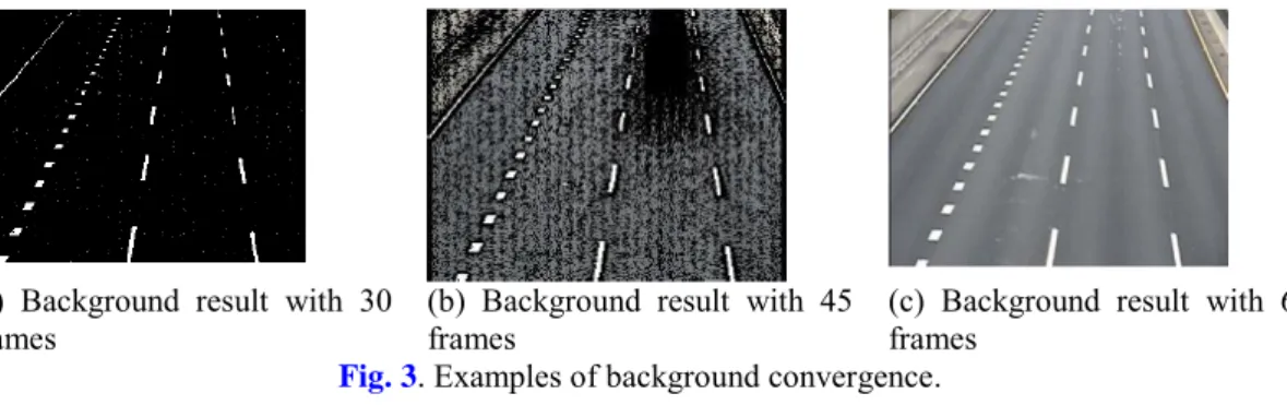
(13) Hence, the background can converge according to (14).), , , ( ) , (x y CM x y k BG (14) An example of background converging result is shown in Fig. 3. In Fig. 3-(a), it shows the background result by converging 30 frames. From the experimental result, it is obvious that the color information of the background is not sufficient and so the background is simple. The background result obtained by converging 45 frames is shown in Fig. 3-(b). After 45 frames, the color information of the background is incrementally built. Finally, the background result by converging 64 frames is presented in Fig. 3-(c).
(a) Background result with 30 frames
(b) Background result with 45 frames
(c) Background result with 64 frames
Fig. 3. Examples of background convergence.
3.2 Segmentation of Moving Objects
Once the background has been properly extracted, the moving objects are detected by checking the sum of differences between the background and the input frame with Eq.(15).
,
))
,
(
)
,
,
(
(
)
,
(
, ,
B G R i i ix
y
t
BG
x
y
f
y
x
MSD
(15) where fi(x,y,t) is the input frame in (x,y) at time t, and i = R, G, and B. Next, two parameters, α and β, are used to determine the binary mask MM(x,y) of the moving objects in Eq.(16).
otherwise.
,
0
)
,
(
and
)
,
(
,
1
)
,
(
y
x
MSD
y
x
MSD
y
x
MM
(16)When the background is updated at each frame, the dynamic segmentation with the fixed parameters can overcome the slow changes in illumination caused by variations in daylight or
the weather. However, when the illumination changes rapidly due to AES or other strong interfering noise in the visible spectrum, these fixed parameters will induce false detections. To deal with this, an adaptive thresholding procedure is developed to resolve the rapid changes in illumination. The first step in this procedure is to find the trough VL=[VLR, VLG, VLB,]
T
and the peak VH=[VHR, VHG, VHB,]
T
of the filtered difference distribution FD(n)=[FDR(n), FDG(n), FDB(n)]
T
between the background and the input frame. Second, the filtered difference distribution that depends on a difference distribution in Eq.(17) is obtained by applying Eq.(18). , ] 1 , 1 , 1 [ ) ( T ) , ( ) , , ( ) , ( ) , , ( ) , ( ) , , (
n y x BG t y x f n y x BG t y x f n y x BG t y x fR R G G B B n D (17) . 1 2 ) ( ) (
p i n p n p n i D FD (18) In Eq.(18), 2p+1 is the filter order of the specified moving average filter. The reason for not directly using D(n) to find the valleys is that D(n) may be corrupted by noise. With the filtered difference distribution, the Laplacian operator in Eq.(19) is utilized to find the correct troughs with Eqs.(20) and (21).),
1
(
)
(
2
)
1
(
)
(
2
FD
n
FD
n
FD
n
FD
n
(19)
arg
(
)
0
,
min
2
FD
n
VL
(20)
arg
(
)
0
,
max
2
FD
n
VH
(21)where min(), max(), and arg() are tuple-wise operations.
Finally, the parameters α and β can be obtained using Eq.(22). With these dynamic threshold settings, the dynamic segmentation can overcome the rapid changes in illumination caused by various environment changes.
.
,
B G R B G RVH
VH
VH
VL
VL
VL
(22) Examples of applying the adaptive thresholding procedure to overcome the rapid illumination changes caused by AES are presented in Fig. 4. Fig. 4-(a) shows the originalframe that is affected by AES. If the fixed parameters (α = -25 and β = 25) are applied, there will be some false moving objects segmented as shown in Fig. 4-(b). Moving objects are
segmented correctly in Fig. 4-(c) when applying the adaptive thresholding procedure. When
compared with the experimental results of Fig. 4-(b) and Fig. 4-(c), we find that when AES occurs, some false moving objects are detected due to the effects of light on the application of fixed parameters. However, with the application of the adaptive thresholding procedure, these effects will not impact the segmentation of moving objects. From this example, we can conclude that the adaptive thresholding procedure is a useful method to overcome the changes in illumination.
(a) (b) (c)
Fig. 4. Examples of applying the adaptive thresholding procedure to overcome the rapid changes in illumination caused by AES. (a) The original frame affected by AES. (b) False Moving objects obtained
by applying the fixed parameters. (c) Moving objects obtained by applying the adaptive thresholding procedure.
3.3 Adaptation of the Background to Illumination Changes
Although the adaptive thresholding procedure can be used to overcome the rapid changes in illumination, the extracted background should be smoothly updated to overcome the environmental changes with Eq.(23). This updating makes the extracted background more flexible, helping to overcome the effects of variations in illumination as day turns to night and the changes in light intensity caused by changing weather.
)). , ( ) , , ( ( 1 ) , ( 1 ) , ( x yt x y n y x n n y x BG f BG BG (23)
3.4 Compensation for Background
Although the background extraction process can yield the initial background rapidly and robustly, such initial background may be influenced by some vehicles parked on the roadside during the extraction of background. Once these parked vehicles begin to move away, the moving object segmentation procedure will falsely detect these regions as moving objects. Furthermore, the falsely detected regions of the background will never be updated because the moving-object regions of the background are impossible to update. Accordingly, a background compensation method is proposed to correct these false detections.
The background compensation method adopts a trajectory feedback from the vehicle-tracking process to decide whether the moving objects are falsely detected; if the following three conditions are satisfied, then we determine that particular moving object detection to be false.
I. The centers of the moving objects do not change significantly over a period of time. II. The starting nodes of the trajectories are not close to the boundary of a frame. III. No edge is present near the contour of a moving object.
If these three conditions are met in the trajectories of any moving object, the regions of the moving objects will be recognized as the background.
4. Lane Detections and Prior Split by Lane Mask
In this section, methods of lane detection and prior split by lane mask are presented. They are used to detect lanes and resolve vehicle occlusions automatically in a given detection zone. 4.1 Automatic Detection of Straight Lanes
There are several steps that have to be taken to detect lane markings automatically. First of all, line segments should be extracted. Second, line segments are grouped as lane separators. Next, noise is filtered. Finally, the lane markings are constructed.
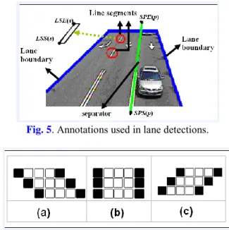
At the beginning of the procedure, the line segments must be extracted. The background BG(x, y) obtained by the process of color background extraction is used to derive a binary image LMC(x, y) with either white or yellow lane markings. The line segment candidate of lane markings shown in Fig. 5 is obtained by using Eq.(24).
)),
(
(min(
arg
)),
(
(max(
arg
,
)
(
)
(
,
)
(
)
(
min maxn
spb
nb
n
spw
nw
i
n
p
n
spb
i
n
p
n
spw
n n M M i B M M i Y
. 0 ), ) , ( ) , ( ( , ) , ( , ) , ( 1 ) , ( min max max max otherwise nb y x BG or nw y x BG and nw y x BG and nw y x BG y x LMC B B G R (24)In Eq.(24), PY(n) is the gray level value at n in the histogram of the Y component. PB(n) is the gray level value at n in the histogram of the B component. 2M+1 is the ordered position of the filter.
Next, each pixel in LMC(x, y) is scanned from left to right, bottom to top to yield the bottom-left coordinate, LSS(s) = (LSSX(s), LSSY(s)), and the top-left coordinate, LSE(s) = (LSEX(s), LSEY(s)), of the s
th
straight line segment. LSS(s) is defined as the coordinate of a start point. Three types of vertical connection displayed in Fig. 6 are applied to search LSE(s) with the following steps.
I. Assign LSE(s) as LSS(s).
II. Find out if one of the following coordinates is a start point: (LSEX(s) - 1, LSEY(s) – 1), (LSEX(s), LSEY(s) – 1), and (LSEX(s) + 1, LSEY(s) – 1).
III. If the start point exists, assign LSE(s) to the coordinate of the start point and go to step II.
IV. Otherwise, set s to s + 1.
During the scanning, each scanned pixel is marked with a processed flag so that it won’t be reprocessed. After all line segments are determined, a line segment merging procedure will be applied to group line segments into separators lane by lane as shown in Fig. 5. Assume the start and the end coordinates of the pth separator shown in vector form are defined as SPS(p) = [SPSX(p),SPSY(p)]
T
and SPE(p) = [SPEX(p), SPEY(p)]
T
, respectively. All line segments belonging to the separator should have similar slopes. The first step in grouping the separators is to calculate the slopes of all the line segments. The next step is to extend a separator for each line segment from the top to the bottom of the image. Line segments near the extending separator with similar slopes should be grouped into the separator. Finally, all separator candidates will be determined, when all line segments are checked.
Finally, horizontal and vertical noise should be removed by utilizing the characteristics of position and height. If any two boundaries caused by double lines or just noise are too close geometrically, the one nearest to the boundary of the detection zone will be removed.
Examples of filtering horizontal and vertical noise are shown in Fig. 7.
Fig. 5. Annotations used in lane detections.
Fig. 6. Vertical connection types: (a) Left hand (b) Front (c) Right hand.
(a) (b) (c) (d)
Fig. 7. Examples of removing horizontal and vertical noise. (a) Original background image. (b) A binary image before removing noise. (c) A binary image after removing horizontal noise. (d) A binary
image after removing vertical noise. 4.2 Prior Split by Lane Mask
If vehicles are occluded as they are just entering the frame, it will be difficult for the tracking process to create correct tracking trajectories. When the process of moving object segmentation cannot split such occlusions, a splitting approach will be necessary to resolve the occlusion before applying the tracking process. In this paper, a lane mask as described in the previous section is used as a reference for separating occluded vehicles. This approach is based on the assumptions that most vehicles are occluded horizontally when they are moving vertically in adjacent lanes. The proposed prior occlusion detection and resolution method is described as follows.
Before detecting vehicle occlusions, the label ID l and the label ID image g(x, y) of a moving object are obtained by applying connected-component labeling [17] together with the use of the lane mask LM(x, y). The values of LM(x, y) are defined as: -1 (ignored), 0 (separators or boundaries), 1 (first lane), 2 (second lane), and so on.
In the scheme to perform occlusion detection, each pixel of the lth moving object is checked to determine whether the pixel should be accumulated into a histogram with Eq.(25).
, 1 )) , ( , ( )) , ( , (l LM x y S l LM x y S
Where
.
0
)
,
(
and
1
)
,
(
and
)
,
(
y
x
LM
y
x
LM
l
y
x
g
(25)Furthermore, another histogram ST(l, h) based on a lane ID h with the top-most coordinate T(l) and the bottom-most coordinate B(l) of the lth moving object is given by Eq.(26).
.
0
)
,
(
and
1
)
,
(
and
1
))
,
(
,
(
))
,
(
,
(
y
x
LM
y
x
LM
l
B
y
l
T
where
y
x
LM
l
ST
y
x
LM
l
ST
(26)Certainly, each element in the histograms should be set to the initial state. Based on the histograms, the occurrence of occlusion is detected when Eq.(27) is satisfied.
.
5
)
1
,
(
)
,
(
and
),
,
(
)
,
(
2
h
l
-S
h
l
S
h
l
ST
h
l
S
(27) For occlusion resolution, the lth moving object is updated through the use of Eq.(28).. 0 ) , ( and ) , ( , 0 ) ( y x LM l y x g if x,y MM (28)
This prior occlusion detection and resolution technique is performed before commencing the tracking of vehicles.
5. Multiple-Vehicle Tracking and the Update of Traffic Parameters
In this section, multiple-vehicle tracking and a strategy to update traffic parameters within the process of rule-based tracking through reasoning are presented. There are several steps involved in tracking multiple vehicles. First, the false moving objects should be filtered; second, the trajectories of the tracked targets should be updated. Also, vibrating moving objects, which appear as noise, need to be eliminated. Finally, algorithms need to be implemented to resolve vehicle occlusions, some proposals for which are presented in this work.
5.1 Filtering of Falsely Detected Objects
Falsely detected objects can normally be eliminated based on the spatial properties obtained by applying connected component labeling. These spatial properties include the top-most coordinate T(l), the left-most coordinate L(l), the bottom-most coordinate B(l), the right-most coordinate R(l), the area A(l), the width W(l), the height H(l), the aspect ratio AR(l), the size S(l), and the density D(l). In the spatial properties listed above, the first five can be directly evaluated while applying connected component labeling, and the others are derived using Eq. (29) to Eq. (33). , 1 ) ( ) ( ) (l Rl Ll W (29)
,
1
)
(
)
(
)
(
l
B
l
T
l
H
(30),
)
(
)
(
)
(
l
W
l
H
l
AR
(31) ), ( ) ( ) (l W l H l S (32).
)
(
)
(
)
(
l
S
l
A
l
D
(33) These spatial properties are employed to filter out the falsely detected objects. In other words, moving objects with spatial properties that fall into an unreasonable range of values will be filtered and eliminated as noise.5.2 Updating Trajectories and Eliminating Vibrating Moving Objects
The centers of the trajectories are adopted as the reference point to correlate current moving objects with their trajectories and to reduce the computational burden. Euclidean distances between the center of the moving object and the last trajectory node are used to determine if a moving object can be correlated with an existing trajectory. If the number of nodes (tracking count) in the current trajectory exceeds one, the angle of the lth moving object is checked with Eq.(36) to filter noises.
), 1 , ( ) ( ) , , (l k t C1l C2k t P (34) ), 2 , ( ) 1 , ( ) , (k t C1k t C2k t Q (35) ), cos( ) , ( ) , , ( ) , ( ) , , ( ) , , (l k t l k t k t l k t k t AC P Q P Q (36) where C1(l) is the center of the lth moving object, and C2(k,t) is the center of a node in the kth trajectory at time t.
In Eq.(36), if AC(l, k, t) > 0, the lth moving object must satisfy the angular constraint θ with the kth trajectory at time t. If a moving object satisfies the distance constraint but does not satisfy the angular constraint, a variations counter associated with the trajectory will be accumulated. If the variations counter of the trajectory exceeds a certain value, the trajectory will be classified as that belonging to a vibrating moving object, and the trajectory will be ignored as noise.
5.3 Resolving Multiple-Vehicle Occlusions
Any detected moving objects that cannot be correlated to an existed trajectory should be checked to see if it is occluded. A method is proposed to split vehicles occluded in the middle of a frame. The steps used to perform the splitting are as follows:
Step 1: Check the intersection region of the bounding box of the current moving object and the estimated bounding box of the last trajectory node. If the intersection is not empty, then go to step 2. As the estimated bounding box is derived by the last and the penultimate trajectory nodes, the kth trajectory, which spans less than 2 nodes at the current time, will not split. Step 2: Calculate the area of intersection TG(l) of the lth moving object area and the estimated area of the kth trajectory’s last node within the bounding box obtained in step 1. Then, if the intersected area TG(l) divided by the total area of the last node is sufficiently small, the moving object will be regarded as not occluded. Otherwise, go to step 3 to split the moving object.
Step 3: As the number of occluded vehicles that form a moving object is unknown, if the value of (A(l)-TG(l))/A(l) is less than a reasonable value, the moving object may consist of a single vehicle. Otherwise, the moving object may be merged with multiple vehicles, and it may be missed. The merged objects should be split into two newly generated moving objects. One of these two replaces the original moving object and the other is added to the end of moving object list. The second moving object will be checked again by repeating steps 1 to 3.
Fig. 8 shows examples of tracking multiple vehicles. The original frame is shown in Fig.
8-(a). Fig. 8-(b) shows the moving object mask obtained by applying dynamic segmentation.
Fig. 8-(c) depicts the moving object candidates by applying connected-component labeling
and filtering falsely detected objects. Fig. 8-(d) shows the bounding boxes of vehicles (in red) and the 6 most recent trajectory nodes (in magenta) in the original frame.
(a) (b) (c) (d)
Fig. 8. Examples of tracking multiple vehicles. (a) Original image. (b) Moving object mask. (c) Colorful representation of connected components after applying Connected Component Labeling. (d)
Tracking trajectories obtained. 5.4 Calculation of Traffic Parameters
Most traffic parameters can be derived from the tracking trajectories. Table 1 presents the
equations used to calculate the traffic parameters. These parameters are updated when the tracked object moves out of the frame and its trajectory is deleted from the tracking list.
Table 1. Equations used to calculate traffic parameters
Traffic Parameters Equations
Speed: VS(h*) ( ) 005 . 0 ) 1 , ( )) 1 , ( , ( ) 1 , ( 8 7 )) , ( ( 8 1 )) , ( ( * * k W FPH t k N t k N t k t k t k h VS t k h VS C C ,
where FPH is the number of frames per hour; N(k, t) is the number of nodes in the kth trajectory at time t; C(l) is the center of the lth moving object;
W
(k
)
is the average width of nodes in the kth trajectory. Quantity: VQ(h*) If N(k, t-1) > 3, thenVQ(h*(k, t))=VQ(h*(k, t))+1
Headway: H(h*)
First, initialize tH (h) = 0 for all lane ID h. )) , ( ( )) , ( ( )) , ( ( * * * VSh kt FPH t k h t t t k h VH H tH (h*(k, t)) = t Volume: VV(h*) t FPH t k h VQ t k h VV( ( ,)) ( ( ,)) * * Occupancy: VO If N(k, t-1) > 3, then
1
OF
OF
% 100 t OF VO
6. Experimental Results
The experimental results are obtained by testing several scenarios as shown in Fig. 9. The size of each image is 320 × 240 and the sampling rate of the sequence is 30 fps. In Fig. 9-(a) and
Fig. 9-(b), there are two different weather scenarios - one being sunny and on the highway, the
other being cloudy in an urban setting. Fig. 9-(c) shows vehicles moving at high speeds with heavy shadowing effects on the highway. The test case in rainy conditions is shown in Fig.
9-(d). Fig. 9-(e), shows one of the tougher test cases, where vehicles moving at night have to
be detected. Finally, test cases in traffic jams are shown in Fig. 9-(g). The testing conditions for each testing scenario are listed in Table 2. In Table 2, HC is the height setting of the camera, and the viewing angle is θC. CTF is the traffic flow per hour, and VM is the average velocity of each car during testing. TAP is the average processing time per frame. The proposed system is developed on a Windows XP platform with a Pentium-4 2.8 GHz CPU and 512M RAM. In
Table 2, the average processing time per frame with a resolution of 320 × 240 in various environments is less than 13ms, which achieves 76 frames per second. With a real time constraint, the computing efforts of the system do not exceed 50% of CPU time, leading to the conclusion that the proposed system can work in real time.
There are four parts to the experimental results. Accuracy ratios for detecting vehicles are addressed in section 6.1. The accuracy ratios for velocity and vehicle classification are presented in section 6.2 and section 6.3. Finally comparisons with other methods are listed in section 6.4.
(a) (b) (c) (d)
(e) (f) (g)
Fig. 9. Test scenarios in various conditions.
Table 2.The testing conditions for each scenario
Scenario HC (m) θC (°) C TF (1/hr) VM (km/hr) TAP (ms) (a) Sunny 12 6 770 90 11.9 (b) Cloudy 6 10 356 34 11.7 (c) Shadow Effects 12 6 725 89 13.4
(d) Rainy 6 10 287 33 12.3
(e) Night Condition 6 10 309 76 11.7
(f)Heavy Traffic 12 10 1135 45 12.7
(g)Traffic Jams 6 6 523 12 12.6
6.1 Accuracy ratio of vehicle detection
Table 3 shows the experimental results for detecting vehicles. The accuracy ratios of the first
two scenarios, (a) and (b), are similarly high. From the results, we may infer that the proposed methods have good detection ratios under the normal weathers. In scenario (c), we can see that the background has heavy shadow effects. However, the test result still has high accuracy ratios. In scenario (d), we can see that average detection ratios of around 95.7% may be achieved even in rainy conditions. In addition, the accuracy ratio at night is around 84.2%. Finally, the results of two traffic jams scenarios tested are presented, and they show that the proposed system can do well in traffic jams, especially on the highway. Besides, in Table 3,
the false alarm counts (FAC, false-positive errors) are quite small in most cases, which is an indicator that the proposed system is robust in the various testing environments.
Table 3. Accuracy ratios for detecting vehicles
Scenario DC/TTC(*) FAC(**) Accuracy Ratio (%)
(a) Sunny 732/743 14/743 98.5%
(b) Cloudy 583/603 21/603 96.7%
(c) Shadow Effects 583/603 21/603 96.7%
(d) Rainy 464/485 17/485 95.7%
(e) Night Condition 406/482 8/482 84.2%
(f) Heavy Traffic 511/556 14/556 97.9%
(g) Traffic Jams 729/789 12/789 92.4%
(*) DC is the Detection Count and TTC is the Total Target Count (**) FAC is the False Alarm Count
6.2 Accuracy ratio of velocity detection
Experimental results for the detection of velocity are shown in Table 4. The initial velocity of the tracking target is calculated from the changes in gravity. After that, the average velocity, denoted as VS, is updated with the speed equation shown in Table 1. The reference velocity is detected by the radar used for velocity detection where the tolerance is set to ±5 kilometers per hour. If the difference between the velocity detected by the proposed system and that detected by the radar is lower than the tolerance, the velocity is taken to be correct. In Table 4, there are two types of accuracy ratios calculated. One is based on total target count (TTC), which is affected by the detection ratios shown in Table 3. Another type is based on the detected count (DC), where the detection ratios become higher than the first type of accuracy ratio. From the results listed in the table, the detection ratios of velocity are high in most cases. In the nighttime scenario (e), the detection ratios are lower than in other cases. That is because the effects of light heavily affect the detection of size and the positions that are calculated based on gravity. In the traffic jam scenario (g), vehicles move slowly and stop suddenly for traffic lights. So the velocities in this case fluctuate heavily and the accuracy ratios are lower than other cases.
Table 4. Accuracy ratio for detecting velocity Scenario DCV/TTC (*) Accuracy Ratio
(%) DCV/DC Accuracy Ratio (%) (a) Sunny 721/743 97.0% 721/732 98.5% (b) Cloudy 576/603 95.5% 576/583 98.8% (c) Shadow Effects 686/711 96.5% 686/696 98.6% (d) Rainy 454/485 93.6% 454/464 97.8%
(e) Night Condition 356/482 73.9% 356/406 87.7%
(f) Heavy Traffic 491/556 88.3% 491/511 96.1%
(g) Traffic Jams 650/789 82.4% 650/729 89.2%
(*) DCV is the correct detection count for velocity 6.3 Accuracy Ratio of vehicle classification
Table 5 shows the accuracy ratios for vehicle classification. There are two types of vehicles to
classify. One type consists of large vehicles including bus and trucks; the other type comprises the small vehicles including sedans and vans. There are major differences between small and large vehicles mainly in the width and the height. From the experimental result in Table 5, the classification results are good except for the cases in rain and at night.
Table 5. Accuracy ratio for vehicle classification Scenario CR/TTC (*) Accuracy Ratio
(%) CR/DC Accuracy Ratio (%) (a) Sunny 682/743 91.8% 682/732 93.1% (b) Cloudy 551/603 91.4% 551/583 94.5% (c) Shadow Effects 640/711 90.0% 640/696 92.0% (d) Rainy 392/485 80.8% 392/464 84.5%
(e) Night Condition 337/482 69.9% 337/406 83.0%
(f) Heavy Traffic 480/556 86.3% 480/511 93.9%
(g) Traffic Jams 688/789 87.2% 688/729 94.3%
(*) CR is the Accuracy Ratio for vehicle classification 6.4 Comparisons with other approaches
Comparisons with other approaches are listed in Table 6. As shown, the detection and tracking ratio in [9] is similar to that obtained with the proposed approach though it does not detect the vehicle velocity and vehicle classifications. Next, not only are the detection ratios and the classification ratio of [14] lower than those with the proposed approach, it evaluates fewer traffic parameters, too. Finally, the detection and tracking ratios in [18] are also lower than those seen with the proposed system, and it calculates less traffic parameters, though it does not classify vehicles.
Table 6. Comparison to other approaches Scenario Type Cucchiara et al.
[9]
Gupte et al. [14] Michalopoulos et al. [18] Proposed Approach (a) Sunny DC 97.9% 92% 96.8% 98.5% DCV N/A N/A 98.2% 98.5% CR N/A 89.2% N/A 93.1% (b) DC 96.2% 92.2% 94.8% 96.7%
Cloudy DCV N/A N/A 96.3% 98.8% CR N/A 90.5% N/A 94.5% (c) Shadow Effects DC 96.5% 91.2% 93.5% 97.9% DCV N/A N/A 96.5% 98.6% CR N/A 91.3% N/A 92.0% (d) Rainy DC 95.4% 94.1% 93.5% 95.7% DCV N/A N/A 96.2% 97.8% CR N/A 82.5% N/A 84.5% (e) Night Condition DC 78.6% 83.2% 81.5% 84.2% DCV N/A N/A 80.2% 87.7% CR N/A 82.1% N/A 83.0% (f) Heavy Traffic DC 97.1% 93.5% 92.9% 97.9% DCV N/A N/A 95.8% 96.1% CR N/A 92.1% N/A 93.9% (g) Traffic Jams DC 93.5% 91.8% 90.3% 92.4% DCV N/A N/A 88.5% 89.2% CR N/A 91.6% N/A 94.3%
The experimental results above show that the proposed approach works well in various complex traffic conditions.
6. Conclusion
This study presents an MVDT system with automated parametric evaluation, vehicle detection, prior splitting based on lane information, vehicle tracking, post splitting, and comprehensive traffic parameter calculation. Initially, color background extraction based on spatiotemporal statistics with luminance adaptation, along with compensation of incorrect convergence is utilized to segment moving objects robustly. Next, prior splitting based on the previously gathered lane information is exploited using an automatic straight lane detection technique to resolve occluded vehicles that are just entering the detection zone. However, some vehicles may be occluded because they happen to be changing lanes in the middle of the detection zone, in which case, a post-splitting approach is applied. Finally, traffic parameters based on tracked trajectories are calculated to build traffic information.
Experimental results indicate that the proposed system operates well in real time. The results also show that the proposed system can work well in various weather and traffic conditions. The precision and reliability of the proposed system is quite good because a lane mask is utilized to help to resolve vehicle occlusion under real-time conditions. Additionally, the developed system can be set up without the need for any information about the environment in advance. Finally, the traffic information that is collected by the proposed system can be used to control traffic, and in combination with a PDA or a mobile phone system it may be used to guide the driver of the vehicle under various traffic conditions. Future works need to improve the accuracy ratio when it is used in a wide range of environments. In addition, detection for motorcycles also needs to be developed to make the system practical for commercial usage.
[1] Yang Wang, “Joint Random Field Model for All-Weather Moving Vehicle Detection,” IEEE
Transactions on Image Processing, vol. 19, no. 9, pp. 2491-2501, 2010. Article (CrossRef Link)
[2] Luo-Wei Tsai, Jun-Wei Hsieh and Kuo-Chin Fan,“Vehicle Detection Using Normalized Color and Edge Map,” IEEE Transactions on Image Processing, vol. 16, no. 3 , pp. 850-864, 2007. Article (CrossRef Link)
[3] Wei Zhang, Q. M. Jonathan Wu and Xiaokang Yang,“Multilevel Framework to Detect and Handle Vehicle Occlusion,” IEEE Transactions on Intelligent Transportation Systems, vol. 9, no. 1, pp. 161-174, 2008. Article (CrossRef Link)
[4] Neeraj K. Kanhere and Stanley T. Birchfield,“Real-Time Incremental Segmentation and Tracking of Vehicles at Low Camera Angles Using Stable Features,” IEEE Transactions on Intelligent
Transportation Systems, vol. 9, no. 1, pp. 148-160, 2008. Article (CrossRef Link)
[5] José Melo, Andrew Naftel, Alexandre Bernardino and José Santos-Victor,“Detection and Classification of Highway Lanes Using Vehicle Motion Trajectories,” IEEE Transactions on
Intelligent Transportation Systems, vol. 7, no. 2, pp. 188-200, 2006. Article (CrossRef Link)
[6] Hsu-Yung Cheng, Bor-Shenn Jeng, Pei-Ting Tseng and Kuo-Chin Fan,“Lane Detection With Moving Vehicles in the Traffic Scenes,” IEEE Transactions on Intelligent Transportation Systems, vol. 7, no. 4, pp.571-582, 2006. Article (CrossRef Link)
[7] Manuel Vargas, Jose Manuel Milla, Sergio L. Toral and Federico Barrero, “An Enhanced Background Estimation Algorithm for Vehicle Detection in Urban Traffic Scenes,” IEEE
Transactions on Vehicular Technology, vol. 59, no. 8, pp.3694-3709, 2010. Article (CrossRef Link)
[8] Jie Zhou, Dashan Gao, and David Zhang, “Moving Vehicle Detection for Automatic Traffic Monitoring,” IEEE Transactions on Vehicular Technology, vol. 56, no. 1, pp.51-59, 2007. Article (CrossRef Link)
[9] Rita Cucchiara, Massimo Piccardi, and Paola Mello, “Image Analysis and Rule-based Reasoning for a Traffic Monitoring System,” IEEE Transactions on Intelligent Transportation Systems, vol. 1, no. 2, pp. 119-130, June 2000. Article (CrossRef Link)
[10] Baoxin Li, Rama Chellappa, “A Generic Approach to Simultaneous Tracking and Verification in Video,” IEEE Transactions on Image Processing, vol. 11, no. 5, pp. 530-544, May 2002. Article (CrossRef Link)
[11] Hai Tao, Harpreet S. Sawhney, and Rakesh Kumar, “Object Tracking with Bayesian Estimation of Dynamic Layer Representations,” IEEE Transactions on Pattern Analysis and Machine
Intelligence, vol. 24, no. 1, pp. 75-89, Jan. 2002. Article (CrossRef Link)
[12] D. M. Ha, J. M. Lee, Y. D. Kim, “Neural-edge-based Vehicle Detection and Traffic Parameter Extraction,” Elsevier, Image and Vision Computing, vol. 22, no. 11, pp. 889-907. Article (CrossRef Link)
[13] Christopher E. Smith, Scott A. Brandt, and Nikolaos P. Papanikolopoulos, “Visual Tracking for Intelligent Vehicle-highway Systems,” IEEE Transactions on Vehicular Technology, vol. 45, no. 4, pp. 744-759, Nov. 1996. Article (CrossRef Link)
[14] Surendra Gupte, Osama Masoud, Robert F. K. Martin, and Nikolaos P. Papanikolopoulos, “Detection and Classification of Vehicles,” IEEE Transactions on Intelligent Transportation
Systems, vol. 3, no. 1, pp. 37-47, Mar. 2002. Article (CrossRef Link)
[15] Chao-Jung Chen, Chung-Cheng Chiu, Bing-Fei Wu, Shin-Ping Lin and Chia-Da Huang, “The Moving Object Segmentation Approach to Vehicle Extraction,” in Proc. IEEE International
Conference on Networking, Sensing and Control, vol. 1, pp. 19-23, Mar. 2004. Article (CrossRef Link)
[16] Bing-Fei Wu, Shin-Ping Lin, Yuan-Hsin Chen, “A Real-Time Multiple-Vehicle Detection and Tracking System with Prior Occlusion Detection and Resolution, and Prior Queue Detection and Resolution” in Proc. of 18th International Conference on Pattern Recognition, pp. 828-831, 2006.
Article (CrossRef Link)
[17] Jenji Suzuki, Isao Horiba, and Noboru Sugie, “Fast Connected-Component Labeling Based on Sequential Local Operations in the Course of Forward Raster Scan Followed by Backward Raster
Scan, ” in Proc. of 18th International Conference on Pattern Recognition, vol. 2, pp. 434-437, Sep. 2000. Article (CrossRef Link)
[18] Panos G. Michalopoulos, “Vehicle Detection Video Through Image Processing: The Autoscope System,” IEEE Transactions on Vehicular Technology, vol. 40, no. 1, pp. 21-29, Feb. 1991. Article (CrossRef Link)
Bing-Fei Wu was born in Taipei, Taiwan in 1959. He received the B.S. and M.S. degrees in control engineering from National Chiao Tung University (NCTU), Hsinchu, Taiwan, in 1981 and 1983, respectively, and the Ph.D. degree in electrical engineering from the University of Southern California, Los Angeles, in 1992. Since 1992, he has been with the Department of Electrical Engineering, where he is a Professor in 1998 and promoted as Distinguished Professor in 2010. His current research interests include vision-based vehicle driving safety, intelligent vehicle control, traffic surveillance systems, multimedia signal analysis, embedded systems and chip design.
Jhy-Hong Juang was born in I-Lan, Taiwan in 1974. He received the B.S. in Control Engineering from National Chiao Tung University (NCTU), Hsinchu, Taiwan, in 1997 and the M.S. degree in the Department of Electrical Engineering and Control Engineering from National Chiao Tung University (NCTU) Hsinchu, Taiwan, in 1999. Now he is the PH.D student in Electrical Engineering, National Chiao Tung University (NCTU). His research interests include image processing, software engineering and pattern recognition.