區間設限資料之統計推論-文獻回顧

(1)

國立交通大學

統計學研究所

碩士論文

區間設限資料之統計推論-文獻回顧

Statistical Inference based on

Interval Censored Data

A Literature Review

研究生：黃祥福

指導教授：王維菁教授

(2)

區間設限資料之統計推論-文獻回顧

Statistical Inference based on Interval Censored Data

A Literature Review

研究生：黃祥福 Student：

Hsiang-FuHuang

指導教授：王維菁教授 Advisor：Dr. Wei-Jing Wang

國立交通大學

統計學研究所

碩士論文

A Thesis

Submitted to Institute of Statistics

College of Science

National Chiao Tung University

in partial Fulfillment of the Requirements

for the Degree of

Master

in

Statistics

May 2011

Hsinchu, Taiwan, Republic of China

中華民國一百年五月

(3)

i

區間設限資料之統計推論

研究生：黃祥福指導教授：王維菁教授

國立交通大學理學院

統計學研究所

摘要

在此論文中,我們回顧區間設限資料的推論問題,為呈現概

念的建構原則,亦簡述其它類型的不完整資料.論文分兩大部份,

一部份為無母數估計,另一部份為迴歸分析.我們回顧了兩類的

無母數估計法,其中自我一致演算法可視為動差法的延伸.另一

方法為無母數最大概似估計法.我們介紹三種較廣泛使用的迴歸

模型: 包含比例風險模型,加速失敗模型和比例勝算模型.推論

的困難度在於模式存在未知函數,需要利用平滑的技巧處理之.

本論文以介紹點估計的概念為主,並未涵蓋如何由分佈理論推導

信賴區間與統計檢定問題.

關鍵字:區間設限, 無母數

(4)

ii

Statistical Inference based on

Interval Censored Data

Student：Hsiang-Fu Huang Advisor：Dr. Wei-Jing Wang

Institute of Statistics

National Chiao Tung University

Hsinchu, Taiwan

Abstract

We review inference methods for analyzing incomplete data with

focus on interval censored data. For nonparametric analysis, two

estimation approaches are examined. Self-consistency can be viewed

as an extension of the method of moment by imputing incomplete

information by its expected value. The other is the nonparametric

likelihood estimation. We also introduce three popular regression

models, namely the proportional hazards model, accelerated failure

time model, and proportional odds model. These models contain

unknown nuisance functions and different smoothing techniques are

employed to handle them in the estimation procedure. The thesis

focuses on point estimation so that second ordered properties are not

investigated.

(5)

iii

致謝

很榮幸能夠成為王維菁教授的指導學生,在跟老師寫論文的這

一年當中,老師總是不餘遺力的教導和督促我們.天性散漫的我受到

老師的影響,態度也變得較積極.在課業方面,老師除了幫忙解惑之外,

還訓練我如何去找問題的核心所在,進而去尋找解決問題的方法.這

讓我從一味只會全盤接受他人的想法,慢慢的進步到去思考別人的想

法的正確性,對我的獨立思考能力有相當的幫助.此外,表達能力也是

老師教學的重點.這些都是我先前相當缺乏的能力.雖然我在碩二這

一年沒有修課,但是有這些訓練,讓我覺得比在課堂上學的更多.相信

在之後的職場上也有很大的幫助.

此外也要特別感謝李博文學長和蘇健霖學長對我論文的協助,

我的論文才能在時間內順利完成.

黃祥福僅誌

中華民國一百年夏

于交通大學統計學研究所

(6)

iv

Chapter 1. Introduction

1.1 Motivation

In survival analysis we are interested in studying the behavior of the time to the event of interest, denoted as T , which often cannot be completely observed. Textbooks on survival analysis focus on right censored data in which many elegant results have been derived. In the thesis, we consider interval censored data. Although such data are commonly seen in practical applications, related statistical methods are not formally taught in the classroom. The lack of an overall review at the introductory level provides the motivation of the thesis.

To enhance a thorough understanding about the methodology, we will still review related materials for complete and right censored data and address how the basic ideas are modified when the data become interval censored. We will consider two types of applications. One is nonparametric analysis of the survival function Pr(T t). The other is regression analysis. Specifically let Z be the covariate vector which provides individual information. A regression model imposes additional assumptions on how Z affects T . We will review statistical methods for the proportional hazards (PH) model, the accelerated failure time (AFT) model and the proportional odds model when T is subject to interval censoring.

1.2 Different types of incomplete data

It is worthy to introduce different types of incomplete data and compare their differences.

(1). Right censored data

Observed variables can be expressed as

( , )

X



where X  T C and

( )

I T C

   . Thus when





1

, X T and X C; when





0

, X C and

X T (the true failure time T is located in the right-hand side of the observed time

(8)

2

Most literature in survival analysis consider right censored data.

(2) Left censored data:

We use the same notations to denote observed variables which have different definitions. One observes

( , )

X



where X  T C and  I T( C) . When

1 



, X T and X C; when





0

, X C and X T (the true failure time T is located in the left-hand side of the observed time X ). Here is an example of left censoring. Denote T as the time until first marijuana use among high school boys in California. If the event had already occurred prior to the recruitment of the study, the subject is said to be left censored.

(3) Doubly censored data

Doubly censored data include three types of observations, namely “observed”, “right censored” and “left censored” ones. Let C be the right censoring variable and _r

l

C be the left censoring variable. It is assumed that C_l C_r. Observed variables are

( , )

X



where X max(min(C T C_r, ), _l) and





1

if X T;





0

if X C_r; and



 

1

if X C_l.

(4) Interval censored data

The observation is a random interval ( , ]L R such that T falls in the interval but its exact value is unknown unless LR. Such data can include right censoring if

R  and left censoring if L0. Interval censored are commonly seen in practice. For example a subject is under study has a regular appointment schedule (say every three months) to the hospital. The left endpoint L refers to the last follow-up time that the event has not occurred and the right endpoint R refers to the first follow-up time that the event is detected.

(9)

3

1.3 Parametric analysis for interval censored data

The thesis focuses on nonparametric and semi-parametric methods. However these methods are still motivated by the parametric approach. Here we briefly summarize the parametric analysis for interval censored data denoted as {( ,L R_i _i] (i1,..., )}n . Assume that the distribution function of T is specified as

( )

F_  . The likelihood function and the log-likelihood function can be written as

1 ( ) [ ( ) ( )] n i i i L  F R_ F L_  



 ( 1 . 1 ) and 1 log ( ) log{ ( ) ( )} n i i i L  F R_ F L_  



 . (1.2)

The resulting score function is

1 log ( ) ( ) ( ) ( ) ( ) ( ) n i i i i i L f R f L S F R F L             



 . (1.3)

By solving S( ) 0, we obtain the maximum likelihood estimator of  . Our analysis implies that parametric inference is straightforward for interval censored data. In fact, difficulties arise when the functional form of F( ) is completely unspecified as in the nonparametric setting or partially specified as in the semi-parametric setting.

1.4 Organization of the Thesis

Chapter 2 considers non-parametric inference and Chapter 3 to Chapter 5 discuss semi-parametric regression models, namely the proportional hazards (PH) model, the accelerated failure time (AFT) model and the proportional odds (PO) model respectively. Chapter 6 gives a brief summary of the thesis.

(10)

4

Chapter 2. Inference based on Nonparametric Analysis

The major objective is to estimate the survival function S t( )Pr(T t)

without specifying the parametric distribution. We will review nonparametric methods based on several data structures, from the simplest to the complicated data settings. This will help us to understand the fundamental techniques more thoroughly.

2.1 Complete data

Complete data are denoted as { (T i_i 1,..., )}n which form a random sample of

T . Based on the fact that S t( )E I T[ ( t)] and applying the method of moment, one can estimate it by the empirical estimator

1 1 ( ) ( ) n i i S t I T t n  



 . Although the method of moment provides a simple solution, it does not guarantee any optimality property. Formally the nonparametric likelihood estimator should be pursued as a better option. The first step is to re-write the likelihood function based on grid points and the probabilities at these points are the parameters to be estimated. Suppose that there are only M distinct observed values denoted as t₍₁₎ ... t₍_M₎. Let

( ) 1 ( ) n j i j i d I T t 





 be the number of observations at t_{( )}_j and p_j S t( _{( )}_j  ) S t(_{( )}_j ). The likelihood function can be written as

( ) 1 Pr( ) n j j L T t  



 1 2 1 2 ( ) (d ) ...(d )dM M p p p  . (2.1)

The NPMLE is the solution which maximizes L p( ,...,₁ p_M) subject to

1 1 M j j p  



. Applying the theorem of Lagrange multipliers, let ₁

1 ( ,..., ) log ( 1) M M i i g p p L  p   





and set g p( ,...,₁ p_M)0 Hence the Lagrange equation system is given by

1 0 ( 1,..., ) and 1 M j j j j d j M p p     



 . ( 2 . 2 )

(11)

5

The above equations can be solved easily and the solution is pˆj dj /n for 1,...,

j M and n.

2.2 Right censored data

For right censored data, observed data become {(X_i, ) (



_i i1,..., )}n , where

min( , )

i i i

X  C T



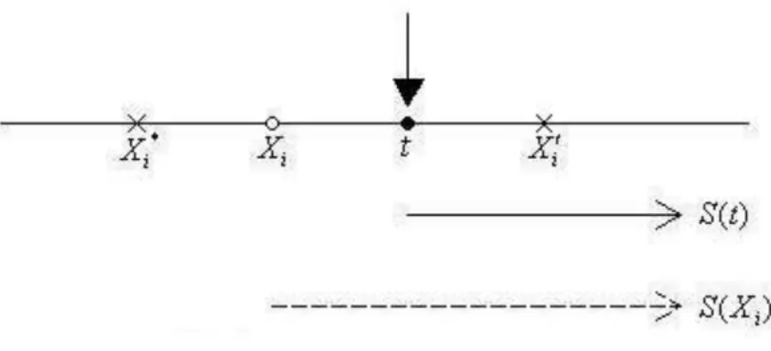
_i＝I T( _i C_i). The survival function can be estimated by the Kaplan-Meier estimator ( , 1) ˆ( ) 1 ( ) i i i u t i i I X u S t I X u          _  _     





_

. The above product-limit expression is elegant since the censoring effect is cancelled out in estimation of the hazard function. However under other types of censoring mechanism, estimation of the hazards does not provide any advantage. Instead, the techniques of self-consistency and nonparametric MLE can be generalized to other data structures. Now we illustrate the self-consistency algorithm for right censored data. The self-consistency equation can be written as

1 ˆ 1 ( ) ˆ( ) ( ) ( , _{0) ˆ} ( ) n i i i i i S t S t I X t I X t n   S X    _     _  







1 1 ( ) (1 ) ( ) n i i i i i I X t I X t w n   



    . (2.3)

Notice that for points with Xi t, the full weight 1 is assigned; for points with i

X t and _i 1, zero weight is assigned; and for points with X_i t and _i 0, partial weight w_i S tˆ( ) / (S Xˆ _i) is assigned. The estimator can be solved successively and explicitly. Since S Xˆ( ) 1_i  for X_i t₍₁₎ with i 0, we have

(1) ˆ( ) S t



₍₁₎ ₍₁₎ ₍₁₎



1 1 _ˆ ( ) (1 ) ( ) ( ) n i i i i I X t I X t S t n   



   

(12)

6

which allows us to solve S tˆ( )₍₁₎ and then successively for S tˆ( )_{( )}_j j2,...,M.

Figure 2.1 Self-consistency for right censored data.

Weight for X_i= 1; weight for X_i = ( ) (S t S X_i); weight for X_i* = 0

Now we discuss the nonparametric MLE approach for right censored data. Define t₍₁₎ ... t₍M₎ as distinct observed failure times and {x(j1),...,x(jm j)} as

ordered censored points in the interval [t_{( )}_j ,t₍_j₁₎). Also let ( ) 1 ( , 1) n j i j i i d I X t   



  and _{( )} ₍ ₁₎ 1 ( [ , ), 0)) n j i j j i i m I X t t   





  . The likelihood function can be written as

( ) ( ) 1 1 Pr( ) ( ) j j d m M j jl j l L T t S x     



_  _



. ( 2 . 4 )

Since the survival function S t( ) is an non-increasing function, we can make the likelihood function larger when ( ₍ ₎)

l

j

S x is replaced by S t(_{( )}_j )¸This suggest that we can instead consider

* ( 1) ( ) ( ) 1 ( ) ( ) ( ) j j d M m j j j j L S t _ S t S t      



_  _{ } _ .

(13)

7

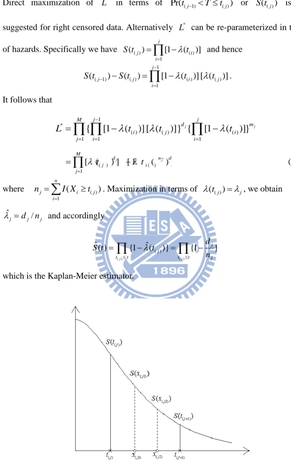
Direct maximization of L in terms of * Pr(t₍j₁₎ T t_{( )}j ) or S t(( )j ) is not suggested for right censored data. Alternatively L can be re-parameterized in terms *

of hazards. Specifically we have _{( )} _{( )}

1 ( ) [1 ( )] j j i i S t  t  



 and hence 1 ( 1) ( ) ( ) ( ) 1 ( ) ( ) [1 ( )] [ ( )] j j j i j i S t S t  t  t     



 . It follows that 1 * ( ) ( ) ( ) 1 1 1 { [1 ( )] [ ( )]} {j [1 ( )]} j j j M d m i j i j i i L



t



t



t     

 





 ₍ ₎ _{( )} 1 [ ( ) ] [ 1j ( j ) ]j M d n d j i j t t     



 (2.5) where _{( )} 1 ( ) n j i j i n I X t 





 . Maximization in terms of (t_{( )}_j )_j, we obtain

ˆ _/ j dj nj   and accordingly ( ) ( ) ( ) ˆ_{( )} _{1 ˆ₍ _)} _{1 _} j j j j t t t t j d S t t n    



 



 which is the Kaplan-Meier estimator.

(14)

8

2.3 Double censored data

Recall that observed data can be denoted as: {(X_i, ) (



_i i1,..., )}n , where

max{min( , ), }

i ri i li

X  C T C and



_i  1 if X_i C_li ;



_i 1 if X_i T_i and 0

i

  if Xi Cri. The self-consistency equation can be written as

1 1 ˆ( ) ( , 1) n i i i S t I X t n   



  ( , 1) ˆ( ) ˆ( ) ˆ 1 ( ) i i i i S t S X I X t S X        ˆ( ) ( , _{0) ˆ} ( ) i i i S t I X t S X     . ( 2 . 6 )

Turnbull (1974) suggested the following steps to implement the algorithm. First, partition the observation period: (0,t₍₁₎], …,(t₍_M_₁₎,t₍_M₎], where t₍₁₎  ... t₍_M₎ are ordered time points. Then define three types of observations in each interval

(1) ( 1) ( ) 1 ( ( , ], 1) n j i j j i i N I X t  t  



   , ( 1) ( 1) ( ) 1 ( ( , ], 1) n j i j j i i N  I X t  t  



    (0) ( 1) ( ) 1 ( ( , ], 0) n j i j j i i N I X t  t  



   .

Turnbull’s idea is to combine “exact” and “left censored” observations by imputation. Specifically for a point in (t₍_k_₁₎,t_{( )}_k ] with   1, the conditional probability of falling in (t₍_j_₁₎,t_{( )}_j ] (for all k  j) is

( ) ( 1) ( 1) ( ) ( ) ( ) ( ) ( ) ( ) ( ) ( ) 1 ( ) j j j j kj k k F t F t S t S t F t S t         .

Thus the imputed value ₍ ₁₎ _{( )}

1 ( ( , ]) n i j j i I T t _ t  



is given by (1) (1) ( 1)_ˆ k m j j k kj k j N N N      



.

(15)

9

(1) (0)

(Nj ,Nj )(j1,..., )m which contains “pseudo-exact” and “right censored” points.

Turnbull (1974) suggested to use them to estimate the hazard probability in the interval (t₍_j_₁₎,t_{( )}_j ] by N(1)_j /Y_j where (1) (0) k m j k k k j Y N N  





 denotes the number at risk and N(1)_j denotes the number of failure. The product-limit expression gives a direct relationship between the survival function and the hazard probabilities:

(1) ( ) ˆ( )_j {1 _i / }_i i j S t N Y  



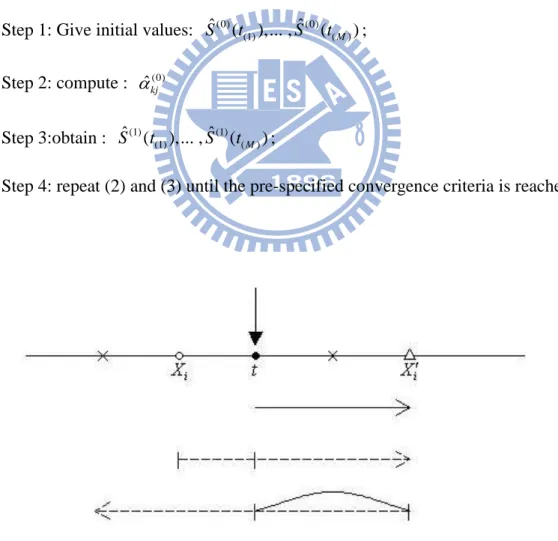
 ( 2 . 7 ).

Note that since both N(1)_j and Y_j are still functions of S tˆ( ),...,₍₁₎ S tˆ(₍_M₎), iterations are needed which can be summarized by the following steps.

Step 1: Give initial values: Sˆ ( ),...(0) t(1) (0) ( ) ˆ ,S (tM ); Step 2: compute : ˆ_kj(0) Step 3:obtain : Sˆ ( ),...(1) t(1) (1) ( ) ˆ ,S (tM );

Step 4: repeat (2) and (3) until the pre-specified convergence criteria is reached.

Figure 2.3 Self –consistency for double censored data

(16)

10

We discuss the NPMLE approach for doubly censored data. The following result is summarized form the work of Mykland and Ren (1996). Let the log-likelihood function of complete data be

1 l o g ( ) n c i i l P T t  



 ( 2 . 8 )

When the failure time ( ,...,T₁ T is known, the NPMLE is easy to obtain as in _n) section 2.1. But under doubly censoring, we cannot observe all the failure time. Hence the EM algorithm is applied. To obtain the iteration, we need to calculate

0 0 ( ) 1 ( | ) [log ( ) | , ] n P i i i i Q P P E P T t X   





where P0 is the initial distribution of T . Here we do not group the observed data as

in Turnbull(1974). Instead, we assume that the distribution of T has mass only at each observations X₍₁₎  X_{( )}_n . Then we discuss the following conditions.

(1) 0[log ( ) | ( ), ( ) 1] log ( ( )) P i i i i i E P Tt X    P TX (2) ( ) ( ) 0 (0) ( ) ( ) ( ) (0) [log ( ) | , 0] log ( ) i j X X j P i i i j i E P T t X P P T X

S

     



(3) ( ) () 0 (0) ( ) ( ) (0) ( ) [log ( ) | , 1] log ( )

1

i j X X j P i i i i j E P T t X P P T X

S

      





where (0) i P and (0) i

S is the initial probability and survival at X_{( )}_i , respectively. Hence for all distinct points w₁w₂ w_M of the set {X₍₁₎  X_{( )}_n},

(0) ( ) 0 ( ) (0) 1 ( | ) ( 1) log ( ) ( 0) log ( ) i j j n i i i i i j i Q P P I P T X I P P T X

S

       _       



(0) (0) ( ) ( 1) log ( )

1

j i j i i j I P P T X

S

       _   





(17)

11 ( ) ( ) (0) (0) 1 1 ( 0, ) ( 1) i n n i j i j j i _i I X X I P

S

        _   



( ) ( ) (0) ( ) (0) 1 ( 1, ) log ( ) i n i j j j i _i I X X P P T X

S

       _  



( ) (0) (0) 1 1 ( _i 0, ) M n i k k k k k i _i I X w P

S

         _  



( ) (0) (0) 1 ( 1, ) log ( ) i n i k k k k i _i I X w P P T w

S

        _  



where _{( )} 1 ( , 1) n k i k i i I X w    



  , _{( )} 1 ( ) n k i k i I X w   



 and 0 0 ( ) k k P P T w . For simply the exception Q P P( | 0) we define

( ) ( ) ( ) (0) (0) (0) (0) 1 1 ( _i 0, ) ( _i 1, ) n n i k i j k k k k k k i _i i _i I X w I X X P P

S

              







and ( _k) _k 1,..., P Tw q k M

Hence Q P P( | ₀) can be re-expressed as

1 log M k k k q  



. Then the M-step is given by 1 m a x l o g M k k k q  



subject to 1 1 M k k q  



(2.9)

Applying the theorem of Lagrange multiplier, the maximization is attained at

ˆ

_k _k

/

1,...,

q





n k



M

.

The steps of iterations are summarized below:

Step 1: set

q

ˆ

_k(0)



1/

M

(

k



1,...,

M

)

; Step 2: set

q

ˆ

_k( )i





_k

/

n

(

k



1,...,

M

)

;

(18)

12

2.4 Interval censored data

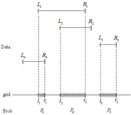
Recall that we observe {( ,L R_i _i] (i1,..., )}n and know that T_i( ,L R_i _i]. Turnbull (1976) discussed nonparametric estimation of Pr(T t) based on interval censored data. The first crucial step is to construct ordered disjoint intervals in which the probability can be estimated. To achieve this goal, the data {( ,L Ri i](i1,..., )}n

are re-arranged in an ascending order and the indentify the intervals such that a left-endpoint and a right-endpoint are adjacent to each other. Denote the disjoint intervals as {( , ] (l r_j _j j1,..., )}m . It can be shown that only these intervals can receive positive mass. Note that an observation ( ,L R_i _i] can occupy more than one intervals ( , ]l rj j for some j . Denote the ij I{( , ]l rj j ( ,L Ri i)} which indicates whether ( ,L R_i _i] overlaps with ( , ]l rj j . Denote pj F r( )j F l( )j as the mass in

( , ]l r_j _j .

The self-consistency equation for an estimator of p_j satisfies

1 1 1 1 1 1 ... n n ij j j ij i i im m i p p w n p p n         



(j1,..., )m ( 2 . 1 0 )

where w can be viewed as the proportion contributed by _ij ( ,L R_i _i]_{in the estimation}

of p_j and hence 1 1 m ij j w  



.

We discuss the NPMLE for interval censored data and see how it relates to the self-consistency solution. The likelihood based on the original data can be written as

1 ( ) ( ) n i i i L F R F L  



 ( 2 . 1 1 ) which can be re-expressed as

(19)

13 * 1 1 n m ij j j i

L



p

 







_

_









where

0 

p

_j



1

and 1

1

m j j

p





. Notice that the summation in

L

* creates numerical difficulty in the maximization. The idea of EM is employed to solve the problem. If the variable

I

_ij



I T

(

_i



( , ])

l r

_j _j can be known, the likelihood based on this “complete” information is given by

* 1 1 ij n m I j i j

L

p

 







_

_





 

and the corresponding log-likelihood is

* 1 1

log

n m ij j i j

L

I

p

 





.

Maximization of

log L

* subject to

1

m j j

p





reduces to the multinomial problem. Applying the theorem of Lagrange multiplier, maximization is attained at

1

ˆ

/

n j ij i

p

I

n





.

However

I

_ij is not known and the “E-step” imputes its value by

1 1 1 ( ,..., ) ... ij j ij m i im m p w p p p p       .

Consequently the “M-step” maximizes

1 1 1

( ,...,

) log

n m ij M j i j

w p

p

 



. ( 2 . 1 2 )

(20)

14 Maximization is attained at 1

ˆ

(

n j ij i

p

w





p

ˆ ,...,

₁

p

ˆ ) /

_m

n

which is equivalent to the self-consistency equation. The steps of iterations are summarized below.

Step 1: set

p

ˆ

(0)_j



1/

m

(

j



1,..., )

m

; Step 2: set ( ) 1

ˆ

(

n k j ij i

p

w





( 1) 1

ˆ

k

,...,

p



p

ˆ

_m(k1)

) /

n

;

Step 3: repeat

k



2,3,...

(Step 2) for until convergence

Figure 2.4 Construction of the mass interval censored data and the idea of self consistency. Weight for( ,L R in estimating₁ ₁] ˆP ,₁ ˆP ,₂ ˆP₃ are 1P₁ (1    P₁ 1 P₂ 0 P₃)

2 1 2 3

1P (1    P 1 P 0 P) and 0 ,respectively.

A different algorithm which directly estimates the survival function was suggested by Turnbull (1976). His idea is based on the product-limit expression of

(21)

15

S(t). The hazard probability in the interval ( , ]l r_j _j can be estimated by d_j/Y_j

where k m j k k j Y d   



and 1 n ij j j i _k ik k p d p   



 

. The algorithm is given below.

Step 1: set (0) 1 n ij j i _k ik

d





 

_, (0) (0) k m j k k j Y d   



(

j



1,..., )

m

Step 2: set ( ) ( ) ( )

ˆ

l

_{1

jl

_}

j l i j j

d

S

Y









_;

(22)

16

Chapter 3. Inference based on Proportional Hazards Model

The proportional hazards model specifies the effect of covariate on the hazard of

T such that 0 1 ( ) lim Pr( [ , ) | , ) Z t T t t T t Z         ₀( ) e x p (t ZT , ) ( 3 . 1 )

where ₀( )t is an arbitrary baseline hazard rate and  is the vector of parameter . The survival function can be written as

exp( )

0 0

( ) exp( t ( ) ) exp( t ( ) exp( T ) ) ( ) Z

Z Z

T

S t  



 u du  



 u Z  du S t 

where S t_Z( )Pr(Tt Z| ). The main objective is to estimate  and usually estimation of 0( )t is of less interest except for the purpose of prediction.

3.1 Inference under right censoring

Right censored data can be denoted as (X_i, ,_i Z_i) (i1,..., )n where i i i

X  T C , _i I T( _i C_i), and Z_i is the covariate. Due to the expression of the likelihood, 1 1 1 ( ) ( ) ( ) i ( ) i i n n Z i Z i i i i i Z Z x S x L f x  S x       _ 



, ( 2 . 2 )

the likelihood function under the PH model can be rewritten as

0 0 0

0 1

) ( ) exp( ) exp( ( ) exp( ) )

( , i i n T T i i x x Z u Z du L

 

      







.

Note that under the semi-parametric setting, the parametric structure of 0( )t is

unspecified.

The partial likelihood approach based on right censored data allows one to estimate  without dealing with ₀( )t . Let t₍₁₎,...,t₍_M₎ be the ordered observed failure times. Let A_i be the set containing the information about who fails at t _{( )}_i

(23)

17

occurs at time t_{( )}_i . The likelihood function can be expressed in terms of the sets

{(A B_j, _j)(j1,...,M)} such that 1 1 2 2 Pr(B A B A ... BM AM)

L

       ( ) ( 1 ) ( 1 ) ( 1 ) 1 P r ( | ) P r ( | ) M j j j j j j j A B A  B B  A   



  ( ) ( 1 ) ( 1 ) ( 1 ) 1 1 Pr( | ) Pr( | ) M M j j j j j j j j A B A  B B  A    









where A( )j (A₁ ... A_j) and B( )j (B₁ ... B_j). Notice that

( ) ( 1) Pr(A B_j | j ,A j ) ( ) ( ) ( ) ( ) ( ) ( ) ( ) ( ) ( ) j k j j j j j k R t z z t dt t dt    



( ) 0 ( ) ( ) ( ) 0 ( ) ( ) ( ) ( ) exp( ) ( ) exp( ) j T j j j T j k j k R t t Z dt t Z dt      



( ) ( ) ( ) exp( ) exp( ) j T j T k k R t z z    



in which 0( )t disappears in the last equation. It can be shown that ignoring the

second component of

L

still leads to an unbiased estimating equation. Specifically the partial likelihood

( ) ( 1 ) 1 ( ) P r ( | ) M j j c j i L  A B A   



 ( ) 1 (_{( )}) exp( ) exp( ) T M j T j k k Rt _j Z Z     

 

( 3 . 3 )

which yields the score function:

( ) ( ) 1 ( ) ( ) ( ) exp( ) ( ) log ( ) exp( ) T k k M _{k R} c j T j k k R j j t t Z Z U L Z Z            



_

.

The estimator of  is the one which solves U( ) 0. Breslow (1975) suggested to estimate ₀ ₀ 0 ( ) ( ) t t  u du  



by

(24)

18 1 0 0 1 ( , 1 ) ( ) ˆ ( ) exp( ) n t i i i n T i i i I X u t I X u Z         







. ( 3 . 4 ) 3.2 Inference under interval censoring

Finkelstein (1986) was the first author to address the inference of proportional hazards models for interval censored data. Observed data can be written as ( ,L R Z _i _i, _i) (i1,..., )n . It is assumed that

T

_i and ( ,L R are independent given _i _i)

i

Z

. The likelihood function can be written as

 

₀

 

₀

 

1 1 [ ( )] { }iT { }iT i i n n Z Z Z i Z i i i i i L S L S R S L  S R      



 



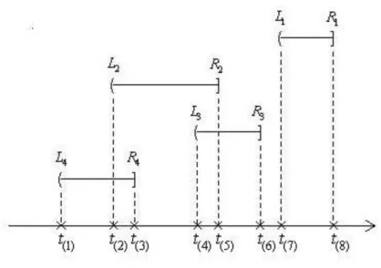
_  _ ( 3 . 5 )

where S t_Z( )Pr(T t Z| ). Unlike the case of right censoring, there is no way to remove S₀(.) from (3.5). This means that we need to estimate  and S₀(.) jointly. The likelihood function in (3.5) is represented based on original observations. For the purpose of maximization when the nuisance function S₀(.) is involved, this function will be expressed in terms of grid points. Figure 3.1 shows the construction of grid points based on an example containing four observed intervals ( ,L R _i _i] (i1, 2,3, 4). In this example, t₍₁₎ t₍₂₎  t₍₈₎ are formed. In general, we let

(0) (1) ( 1)

0t t  t_M_   be ordered grid points. The i th observation to the likelihood (3.5) can be re-expressed as

1 ( 1) ( ) 1 [ ( ) ( )] i i M ij Z j Z j j S t S t     



1 exp( ) exp( ) 0 ( 1) 0 ( ) 1 [ ( ) iT ( ) iT ] M Z Z ij j j j S t  S t      





where _ij 1 if (t₍_j_₁₎,t_{( )}_j ]( ,L R_i _i] and 0 otherwise. Accordingly the likelihood in (3.5) can be written as 1 exp( ) exp( ) 0 ( 1) 0 ( ) 1 1 [ ( ) iT ( ) iT ] n M Z Z ij j j j i L  S t  S t      





 .

(25)

19

Figure 3.1 Construction of the mass interval censored data

Note that S₀(.) is a function but the maximization of L will only be evaluated on its value at the grid points, namely S t₀(_{( )}_j ) for j1,...,M . Since the parameters

0(( )j )

S t for j1,...,M have natural constraint i.e.,0S t₀(₍₁₎) S t₀(₍_M₎) 1 , it

make the mle hard to obtain. Finkelstein (1986) suggested that one can re-parametrize the S t₀(_{( )}_j ) by _k log[ log S t₀(_{( )}_k )]. It can remove the range restriction of the parameters S t₀(_{( )}_j ), but it doesn’t remove the order restriction.

Sun (2006) proposed a corrective method that can remove the nature constraint. The following is the detail of the method. Based on the product-limit expression, one can write 0(( )j ) S t 0 ( ) 0 (1 ( )) j k k t  



   .

Thus L becomes a function of  and  ₀( t₍₁₎),..., ₀( t₍_M₎) . Note that

0( t( )k ) (0,1)

   is a conditional probability. To remove the natural constraint, we can re-parameterize  ₀( t_{( )}k ) by setting

exp( ) 0( ( )) 1 k k t e      .

(26)

20

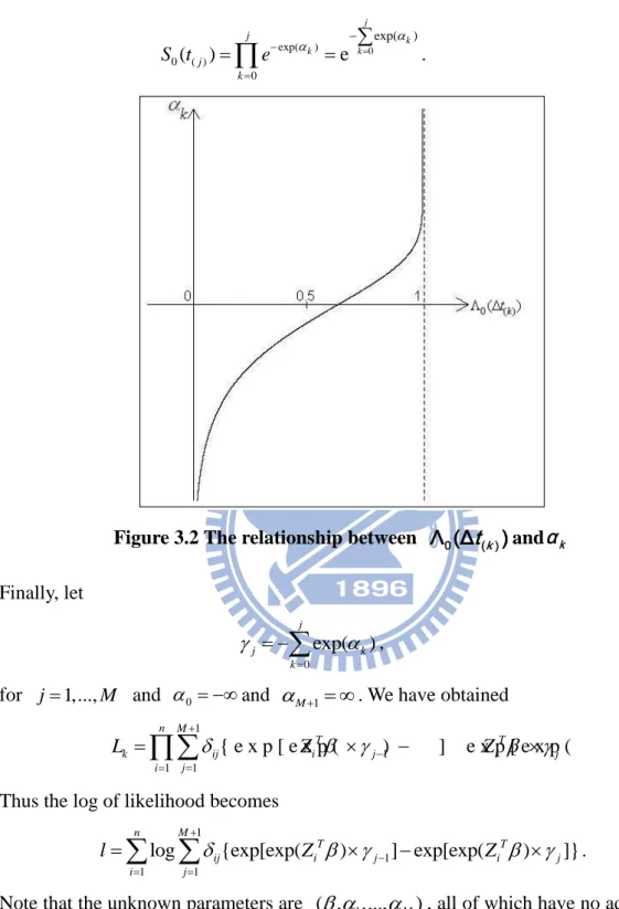
Figure 3.2 shows that by the above transformation,  k  . Thus

0 exp( ) 0 ( ) 0 exp( ) ( ) e j k k k j j k S t e   _    



  .

Figure 3.2 The relationship between Λ (Δ₀ t_{( )}_k )andα k

Finally, let 0 exp( ) j j k k     



,

for j1,...,M and 0  and M1 . We have obtained

1 1 1 1 { e x p [ e x p ( ) ] e x p [ e x p ( ) ] } n M T T k ij i j i j j i L  Z   Z       





   ( 3 . 6 )

Thus the log of likelihood becomes

1

1 1

log {exp[exp( ) ] exp[exp( ) ]} n M T T ij i j i j i j l  Z   Z       

 

   .

Note that the unknown parameters are ( , ₁,...,_M), all of which have no additional constraints. The estimation process is summarized below.

Denote the score statistics as ( , )T T T l l U     

  . The score functions of  and  are given by

(27)

21 1 1 , 1 , 1 1 ( ) n M i i ij i j i j i j l Z g  f f          



and 1 , , 1 n i i j i j i j l g b c      



( j1,...,M ) where 1 ( 1) ( ) 1 [ ( ) ( )] i i M i ij Z j Z j j g  S t S t    



 , _, (_{( )}) log (_{( )}) i i i j Z j Z j f S t S t , fi_,0  fi M_, ₁0, , exp( ) T i j j i b   Z  , 1 , ( 1) _i(( )) M i j ik ik Z k k j c   S t   





 and i m₂ 0. The objective is to

solve U0 so that the likelihood can be maximized. The Newton-Raphson method can be applied to obtain the solution. Let 11 12

21 22

[A A ]

A

A A

 as the observed Fisher information matrix. The elements of A11 include

2 , , , , , , , 2 1 ( ) n i j i k i j i k i j i k i j i j k i i b b c c b b c l g g     _{ } _  



for jk. The elements of ₁₂ ₂₁T A  A include 2 1 1 , 1 , , 1 , 2 , 1 , 1 1 { [ ( ) ] ( )} n M M i j i i j i i j il il i l il i l i l i l j l j i c l Z b g c f f f g               _ _ _ _ _  



.

The elements of A include ₂₂

2 1 1 1 1 , 1 , , 1 , 1 1 1 2 ( ) ( ) n M M T i i i ij i j i j i ij i j i j T j j i l Z Z g  f f g  h h             _ _ _ _ _ _  _ _   



_



_ where , , log _i(( )) , i j i j Z j i j h  f S t  f .

Denote X_n as the estimate of ( , )  in the n -iteration, the Newton-Raphson algorithm can be summarized as follow:

1 1

K K K K

X _ X A U (K 0,1,...),

where A_K and U_K are A and U evaluated at the K th estimate of ( , )  . The procedure is stopped when X_K_₁X_K is close to zero.

(28)

22

Chapter 4. Inference based on Accelerated Failure Time Model

The accelerated failure time (AFT) is a popular alternative to the PH model. An AFT model can be written as

Y ZT  ( 4 . 1 )

where Y logT and  is the error variable with the density function f_(.). Existing research focuses on semi-parametric estimation of  without specifying the form of f_(.). We will briefly review inference methods developed for complete data and right censored data and then focus more on interval censored data.

4.1 Inference based on complete data

Consider the transformed variable under the error scale,  _i( ) Y_i Z_iT for 1,...,

i n. Note that when ₀ is the true value, { ( _i ₀) (i1,..., )}n form an iid sample which becomes a useful property to construct nonparametric inference methods. Let  ₍₁₎( )₍₂₎( )  _{( )}_n ( ) be the order statistics with the corresponding covariates denoted as Z₍₁₎,Z₍₂₎,...,Z_{( )}_n . Define c as the score of _i Z ( )i satisfying 1 0 n i i c  



. Consider the linear rank statistic of the form: _{( )} 1 ( ) n i i i v  Z c  



. ( 4 . 2 )

Note that when   ₀, Pr(Z_{( )}_i Z_k)1/n. As a result,

0 ( ) 1 1 ( ( )) ( ) 0 n n i i i i i E v  c E Z c Z   







 .

This implies that one can estimate  by solving the equation v( ) 0. The error distribution and the form of c both affect the efficiency of the resulting estimator. _i

The Wilcoxon statistic corresponds to 1

2 ( 1) 1

i

c  i n   and the log-rank statistic corresponds to 1 1 1 i j j n   

(29)

23

4.2 Inference based on right censored data

Right censored data are denoted as {(X_i, ,_i Z_i) (i1,2,..., )}n . Let

( ) T

i Yi Zi

    , where Y_i log(X_i). Censored data under the error scale can be written as {( ( ), ) (  _i _i i1,..., )}n . Note that {( (  _i ₀), ) (_i i1,..., )}n form a random sample of { (  ₀), } which is a censored version of  ( ₀). We discuss two methods of modifying the linear rank statistics introduced earlier.

4.2.1 Linear rank statistics

Let  ₍₁₎( )₍₂₎( )  _{( )}_k ( ) be the distinct uncensored ordered error variables and let ₁( ),..., ( )

i

i im

    be censored error variables in _  _{( )}_i ( ),ˆ _{( 1)}_i_ ( )ˆ



. Following the book of Kalbfleisch and Prentice (2002), the modified linear rank statistics can be written as

_{( )} 1 1 ( ) ( ) i m k i i i ij i j v  c Z C Z   







( 4 . 3 )

where Z_{( )}_i and Z_ij represent the corresponding covariates of  _{( )}_i ( ) and  _ij( )

respectively. The requirement is given below:

1 ( ) 0 k i i i i c m C   



.

The efficiency of the resulting estimator depends on the underlying error distribution, the censoring distribution and the forms of c and _i Ci. For the Wilcoxon statistics, Prentice (1978) suggested that

1 1 2 1 i j i j j n c n    



and 1 1 1 i j i j j n C n    



,

(30)

24

4.2.2 Log-rank statistics

As mentioned earlier the log-rank statistics can be expressed as a special linear rank statistics but it has its own representation as follows:

1 1 ( ( ) ( ) ) ( ) ( ( ) ( )) n j i j j LR i i n i j i j I Z U Z I              _         _     



. ( 4 . 4 ) 4.2.3 M-estimator by Ritov (1990)

The idea was motivated by the parametric likelihood analysis. The likelihood function and log-likelihood based on ( ( ), ) (  _i _i i1,..., )n can be written as 1 1 ( , ) ( ( i) ) ( (i ) ) n i i i L  f_ f_    S_     



( 4 . 5 ) and 1 ( , ) log ( ( )) (1 ) log ( ( )) n i i i i i l  f_  f_    S_    



 

respectively. Taking derivative respect to , we get

1 ( , ) ( ( )) ( ( )) [ ( ) (1 ) ( )] ( ( )) ( ( ) n i i i i i i i i i l f f f Z Z f S       _   _ _   _             



.

The difficulty comes from the fact that f , f and S are all unknown functions. The idea of M-estimator is to replace ( )

( ) f f     

 by g( ) which is a known function.

Accordingly l( , f)    can be replaced by ( ) 1 ( ) ( ) ( , ) [ ( ( )) (1 ) ] ( ( )) i n M i i i i i i g u dS u U S Z g S                



 



( 4 . 6 )

where S_( ) can be estimated by the following product-limit estimator

1 1 ( ( ) , 1) ˆ ( ; ) 1 ( ( ) ) n j j j n u t j j I u S t I u                    _  _  _     







.

(31)

25

the resulting estimator. Two common choices of g( ) are g u( )u or

( ) | | . k if u k g u u if u k k if u k      _   _ 

Note that if the error distribution is specified, we have

( ) t f_  



f_ x dx ( ) ( ) ( ) t f x f x dx f x       

_

( ) ( ) t g x dF x   



which suggests the best form of g(.) is (.)

(.) f f   

since it yields the maximum

likelihood estimator.

4.3 Inference under interval censoring

Consider interval censored data ( ,L R Z_i _i_, _i) (i1,..., )n which can be transformed under the error scale such that  _iL( )logL_i Z_iT and

( ) log

R T

i Ri Zi

    . Now we discuss how to extend the ideas of previous methods to interval censored data.

4.3.1 Modify M-estimator by Rabinowitz et al. (1995)

Consider the log-likelihood function

1 ln[ { ( )} { ( )}] n R L i i i L F   F    



 . The MLE of  can be obtained by solving the score function 1 { ( ) } { ( ) } ( ) 0 { ( ) } { ( ) } R L n i i i R L i i i f f S Z F F                  



( 4 . 7 )

and it follows that E S( (₀))0. Since the forms of f_ and F_ are un-specified, one can replace the middle part of S( ) by

[ { ( )}] [ { ( )}] ( , ) { ( )} { ( )} R L i i i R L i i g F g F c F F F                 

where the function g with domain [0,1] satisfies g(0)g(1)0. Thus one can estimate  by solving

(32)

26 1 ( , ) ( , ) 0 n i i i S  F c  F Z  



 .

In Appendix, we show why the restrictions on g makes E S[ (0,F)]0. Again the

form of g(.) and the underlying error distribution affect the efficiency of the resulting estimator. The best choice which leads to the maximum likelihood estimator is g f_ F_1.

Recall that in Section 4.2.3, the nuisance function S_ has an explicit product-limit estimator and hence UM( , Sˆ_(. | )) 0 is solved. However for interval censored data, there is no explicit formula for estimating S_ or F_. One way of estimating F_ is by maxing the likelihood based on

{(   _iL( ), _iR( ))(i1,..., )}n . The grid intervals in which F_ receives masses can be constructed similar to the setup in Section 2.4. Denote t_k( ) (t_kL( ), t_kU( )] for

1,...,

k m as the mass intervals. The next step is to express the likelihood based on

{(   _iL( ), _iR( ))(i1,..., )}n in terms of {(t_kL( ), t_kU( )], k1,..., }m . Define

, ( ) max{ , ( ) : , ( ) ( )}

L

i L j L j L i

t   t  t    and t_{i U}_, ( ) min{t_jR( ) : t_jR( )  _iR( )} . That is (t_{i L}_, ( ), t_{i R}_, ( )] becomes a new representation of (   _iL( ), _iR( )] which will be a union of consecutive t_k( ) . The corresponding log-likelihood function becomes , , 1 ln[ { ( )} { ( )}] n i U i L i l F t_  F t_   



 subject to , , {_{i U}( )} {_{i L}( )} [0,1] ( 1,2,..., ) F t_ b F t_ b  i n and { ( )} [0,1] (_j 1,2,..., ) F t_   j m .

(33)

27

Given an estimate of , the above maximization procedure can be performed. The resulting estimate of F_, denoted as ˆF_, will be plugged into the following

estimating function to solve for the next estimate of : S( ,Fˆ_ ) 1 ˆ ( , ) 0 n i i i c  F Z  



. ( 4 . 8 )

4.3.2 Method for a simplified AFT model with univariate covariate

Besides the methods we discussed earlier, Li and Pu (2003) developed an interesting way to estimate . Consider a simplified AFT model:

i i i i

Y Z  , (i1,...n).

where Zi is a one-dimensional covariate. The main idea of this paper is based on the assumption that _i and Z_i are uncorrelated. Kendall’s provides a rank-invariant measure for assessing the association between two variables. Suppose that ( ,_i Z_i) and ( ,_j Z_j) are independent realizations from ( , ) Z . The pair is concordant if

{( _i _j)( _i _j) 0}

I   Z Z  and discordant if I{( _i  _j)(Z_i Z_j)0}. The population version of Kendall’s tau is defined as

Pr{( _i _j)(Z_i Z_j) 0} Pr{( _i _j)(Z_i Z_j) 0}

           .

The sample estimate of  is

{( )( ) 0} {( )( ) 0} / 2 2 i j i j i j i j i j I Z Z I Z Z n                    



.

If complete data are available, one can solve 1 {( ( ) ( ))( ) 0} {( ( ) ( ))( ) 0} 0 ( 1)i j i j i j i j i j I Z Z I Z Z n n                  



to estimate  . However  _i( ) Y_i _iZ_i is subject to interval censoring such that we only know that  _i( )(   _iL( ), _iR( )]. Some interval observations provide the

(34)

28

complete information for the order of  _i( ) and  _j( ). Notice that if

( ) ( )

R L

i j

    , then  _i  _j.

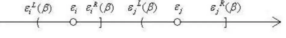
Figure 4.1 The relative position of ε and i ε when j εiR( )β < ε βjL( )

Hence the total number of known concordant pairs becomes

{ ( ) ( R( ) L( )) ( ) ( L( ) R( ))} i j i j i j i j i j I Z Z I     I Z Z I          



and the total number of known discordant pairs is

{ ( _i _j) ( _iL( ) _jR( )) ( _i _j) ( _iR( ) _jL( ))} i j I Z Z I     I Z Z I          



.

The modified Kendall τ coefficient can be write as 1 [ ( ) ( )][ ( ( ) ( )) ( ( ) ( ))] ( 1) R L L R i j i j i j i j i j I Z Z I Z Z I I n n                



.

The resulting estimation function is given by

( ) [ ( ) ( )][ ( R( ) L( )) ( L( ) R( ))] n i j i j i j i j i j K  I Z Z I Z Z I     I      



     

This method has two major drawbacks. One is the restrictive assumption that Z is

univariate. The other is the lack of efficiency if the data contains very few orderable paired intervals.

區間設限資料之統計推論-文獻回顧

國 立 交 通 大 學

統計學研究所

碩 士 論 文