國 立 交 通 大 學
機 械 工 程 學 系
博 士 論 文
動態系統最佳化設計之計算方案與其應用
Computational Schemes for Dynamic System Optimal Design
and its Applications
研 究 生: 黃 智 宏
洪 景 華
教授
指導教授:
曾 錦 煥
教授
動態系統最佳化設計之計算方案與其應用
Computational Schemes for Dynamic System Optimal Design
and its Applications
研 究 生: 黃 智 宏
Student: Chih-Hung Huang
洪 景 華
Ching-Hua Hung
指導教授:
曾 錦 煥
Advisor:
Ching-Huan Tseng
國 立 交 通 大 學
機械工程學系
博士論文
A Dissertation
Submitted to Department of Mechanical Engineering
College of Engineering
National Chiao Tung University
in Partial Fulfillment of the Requirements
for the Degree of
Doctor of Philosophy
in
Mechanical Engineering
May 2006
Hsinchu, Taiwan, Republic of China
動態系統最佳化設計之計算方案與其應用
研究生:黃智宏
指導教授:洪景華 曾錦煥
國立交通大學機械工程學系
摘 要
ABSTRACT (IN CHINESE)
動態系統所引發的特性一直困擾著工程設計人員,而只在靜態系統模式下,採用最佳 化設計方法所求得的設計,則往往在實際的應用上有所不足。本文主要依據最佳設計與 最佳控制理論基礎,結合動態分析與數值分析求解技巧,發展一套通用之動態系統最佳 設計方法與軟體。 一般動態系統之最佳化問題可以轉換成標準的最佳控制問題,再透過離散技術轉換成 非線性規劃問題,如此便可利用現有之最佳化軟體進行求解。在本文中,首先將動態系 統的解題方法與流程發展為最佳控制分析模組,再將該模組與最佳化分析軟體 (MOST) 整合得到整合最佳控制軟體,可以用來解決各種類型的最佳控制問題。為驗證軟體的效 能與準確性,利用本文所發展之整合最佳控制軟體求解文獻資料中所提出之各類型最佳 控制問題。藉由分析結果之數值與控制軌跡曲線的比對,整合最佳控制軟體所求出之數 值解,在效能與準確性上都能與文獻資料所獲得的最佳解吻合,確認該整合最佳控制軟 體的確可以用來解決我們工程應用上的最佳控制問題。 另外,針對工程設計中存在的離散(整數)最佳控制問題,本文依據混合整數非線性 規劃法(mixed integer nonlinear programming) 做進一步的研究。猛撞型控制 (bang-bang type control) 是常見的離散最佳控制問題,其複雜與難解的特性更是吸引諸多文獻探討 的主因。許多文獻針對此一問題所提出的方法多在控制函數的切換點數量為已知的假設
條件下所推導,但這並不符合實際工程上的應用需求,因為控制函數的切換點數量大多 在求解完成後才會得知。因此,本文針對此類型問題發展出兩階段求解的方法,第一階 段先粗略求解該問題在連續空間下的解,並藉此求得控制函數可能的切換點資訊,第二 階段再利用混合整數非線性規劃法求解該問題的真實解。發展過程中,加強型的分支界 定演算法 (enhanced branch-and-bound method)被實際應用並且納入前一階段所開發的整 合最佳控制軟體中,這也使得這個軟體可以同時處理實際動態系統中最常見的連續及離 散最佳控制問題。 最後,本文將所發展的整合最佳控制軟體用來求解兩個實際的工程應用問題:飛航高 度控制問題與車輛避震系統設計問題。兩個問題都屬於高階非線性控制問題,首先利用 本文中所建議的解題步驟建構完成這兩個問題的數學模型,接著直接利用本研究所發展 的軟體求解符合問題要求的最佳解。經由這些實際應用案例的驗證,顯示本文所發展的 方法與軟體的確可以提供工程師、學者與學生一個便利可靠的動態系統設計工具。
Computational Schemes for Dynamic System Optimal Design
and its Applications
Ching-Hua Hung
Student:
Chih-Hung Huang
Advisor:
Ching-Huan Tseng
Department of Mechanical Engineering
National Chiao Tung University
ABSTRACT
The nonlinear behaviors of dynamic system have been of continual concern to both engineers and system designers. In most applications, the designs – based on a static model and obtained by traditional optimization methods – can never work perfectly in dynamic cases. Therefore, researchers have devoted themselves to find an optimal design that is able to meet dynamic requirements. This dissertation focuses on developing a general-purpose optimization method, based on optimization and optimal control theory, one that integrates dynamic system analysis with numerical technology to deal with dynamic system design problems.
A dynamic system optimal design problem can be transformed into an optimal control problem (OCP). Many scholars have proposed methods to solve optimal control problems and have outlined discretization techniques to convert the optimal control problem into a nonlinear programming problem that can then be solved using extant optimization solvers. This dissertation applies this method to develop a direct optimal control analysis module that is then integrated into the optimization solver, MOST. The numerical results of the study indicate that the solver produces quite accurate results and performs even better than those reported in the earlier literatures. Therefore, the capability and accuracy of the optimal control problem solver is indisputable, as is its suitability for engineering applications.
A second theme of this dissertation is the development of a novel method for solving discrete-valued optimal control problems arisen in many practical designs; for example, the bang-bang type control that is a common problem in time-optimal control problems. Mixed-integer nonlinear programming methods are applied to deal with those problems in this dissertation. When the controls are assumed to be of the bang-bang type, the time-optimal control problem becomes one of determining the switching times. Whereas several methods for determining the time-optimal control problem (TOCP) switching times have been studied extensively in the literature, these methods require that the number of switching times be known before their algorithms can be applied. Thus, they cannot meet practical demands because the number of switching times is usually unknown before the control problems are solved. To address this weakness, this dissertation focuses on developing a computational method to solve discrete-valued optimal control problems that consists of two computational phases: first, switching times are calculated using existing continuous optimal control methods; and second, the information obtained in the first phase is used to compute the discrete-valued control strategy. The proposed algorithm combines the proposed OCP solver with an enhanced branch-and-bound method and hence can deal with both continuous and discrete optimal control problems.
Finally, two highly nonlinear engineering problems – the flight level control problem and the vehicle suspension design problem – are used to demonstrate the capability and accuracy of the proposed solver. The mathematical models for these two problems can be successfully established and solved by using the procedure suggested in this dissertation. The results show that the proposed solver allows engineers to solve their control problems in a systematic and efficient manner.
ACKNOWLEDGEMENT (誌謝)
博士論文的完成,首先要感謝及感念的是我的首位指導教授,『最佳化實驗室』的 大家長—曾錦煥教授,沒有他在學術課業上的指導,生活上的照應,待人處事經驗上的 分享,不會有這份論文的完成,僅將此論文獻給來不及在這上面簽名,我亦師亦父亦友 的 曾錦煥博士。 感謝我另一位指導教授 洪景華博士以及齒輪實驗室 蔡忠杓教授,在我們失去曾老 師、頓失依靠之際,毫無保留的給予我們最大的協助,讓這份論文得以順利完成,兩位 老師真心付出,讓學生滿心感激。 對於我的口試委員:清華大學動機系蕭主任德瑛、清華大學動機系宋震國老師、交 通大學機械系學蔡忠杓老師、台灣大學醫學工程研究所呂東武老師與崴昊科技陳申岳老 師,感謝您們不辭辛勞,能撥冗前來指導學生的論文口試,並給予許多適當的指正與寶 貴的建議,使學生的論文內容更加充實與完整。 從民國八十年進入『最佳化實驗室』至今已有15 年,其間與數屆的學長姐、學弟 妹相互學習、討論與砥勉,讓我的學習及研究得以長進,也讓我感受到另一個家庭的溫 暖。在此,我要一併感謝他們,尤其是東武、宏榮與接興等學長們在我學習遭遇挫折與 困頓時給予我極大的鼓勵與支持,在此特別感謝。另外。對於我的同窗好友也是我事業 上的伙伴—寬賢,感謝你在這些年來給予我多方面的協助,讓我能有機會在學術研究之 外,增長實務與管理上的見識。 漫長的學習與研究過程中,需要的除了耐心與努力外,家庭溫暖的親情是支持我堅 持下去的主要動力。從小父母親在南部農村的困頓環境下,縮衣節食,即使四處借貸, 也堅持給我們就學的機會,讓我得以順利取得家族中第一個碩士學位。之後,內人雅惠 在我攻讀博士其間更是無怨無悔的照料家中大小事務,哺育兩個年幼的兒子(國賜與家 富),她長年的包容與等待,讓我可以無後顧之憂,在此論文完成之際,對他們除了感 謝還是感謝!TABLE OF CONTENTS
ABSTRACT (IN CHINESE) ...i
ABSTRACT ...iii
ACKNOWLEDGEMENT (誌謝)... v
TABLE OF CONTENTS ...vi
LIST OF TABLES ...ix
LIST OF FIGURES ... x
NOMENCLATURE...xii
CHAPTER 1 INTRODUCTION... 1
1.1 Dynamic Optimization and Optimization Control Problems ...1
1.2 Literature Review ...2
1.2.1 Methods for Optimal Control Problems ...2
1.2.2 Time-Optimal Control Problems ...4
1.3 Objectives ...5
1.4 Outlines...5
CHAPTER 2 METHODS FOR SOLVING OPTIMAL CONTROL PROBLEMS ...7
2.1 Introduction ...7
2.2 Canonical Formulation of Optimal Control Problems ...9
2.3 First-Order Necessary Condition – Euler Lagrangian Equation ... 11
2.4 Methods for Solving Optimal Control Problems...14
2.4.1 Indirect Methods...14
2.4.2 Direct Methods ...17
2.5 Summary...18
CHAPTER 3 COMPUTATIONAL METHODS AND NUMERICAL PRELIMINARIES FOR SOLVING OCP ... 23
3.1 Introduction ...23
3.2 Nonlinear Programming Problem...25
3.3 Sequential Quadratic Programming Method ...27
3.4 Admissible Optimal Control Problem Method...30
3.4.1 Discretization and Parameterization Techniques...31
3.4.2 Dynamic Constraint Treatments ...34
3.4.3 Design Sensitivity Analysis...36
3.4.4 ODE Solvers for Solving Initial Value Problem...36
3.4.6 Interpolation Functions...38
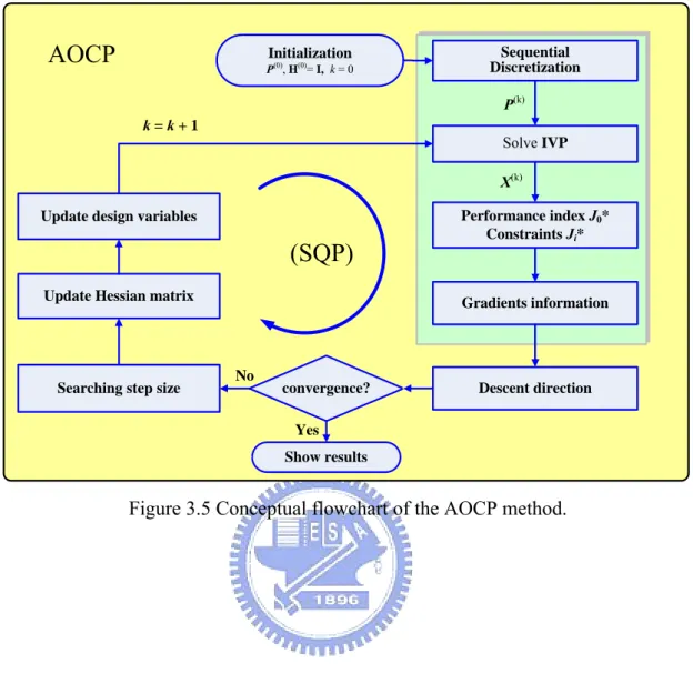
3.4.7 Computational Algorithm of AOCP ...38
3.5 Summary...40
CHAPTER 4 A CONVENIENT SOLVER FOR SOLVING OPTIMAL CONTROL PROBLEMS...47
4.1 Introduction ...47
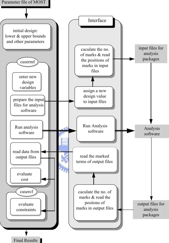
4.2 Multifunctional Optimization System Tool - MOST...47
4.3 Structure of the Proposed OCP Solver ...49
4.4 The OCP Solver in Cooperation with MOST...51
4.5 User Interface for the OCP Solver...52
4.6 Systematic Procedure for Solving the OCP...52
4.7 Illustrative Examples ...53
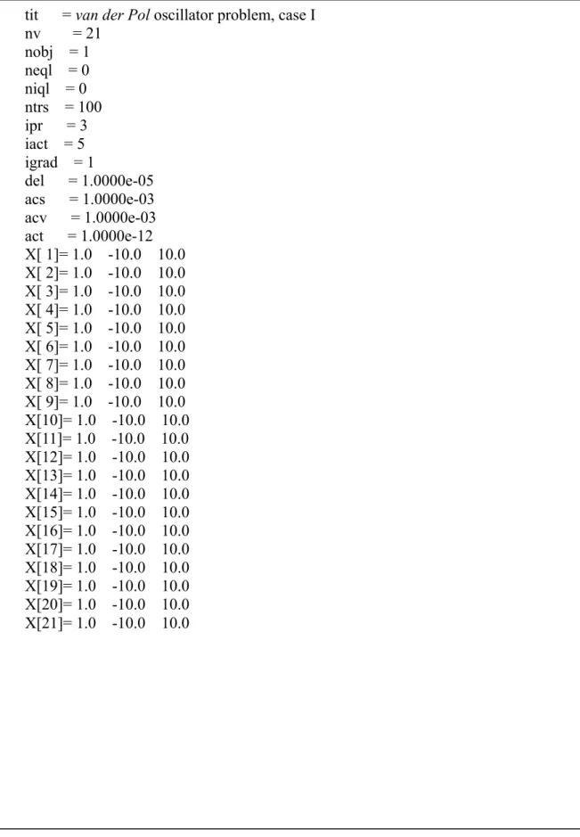
4.7.1 The van der Pol Oscillator Problem ...53
4.7.2 Time-optimal Control Problem: Overhead Crane System...55
4.8 Numerical Study ...58
4.9 Summary...59
CHAPTER 5 A COMPUTATIONAL SCHEME FOR SOLVING THE DISCRETE-VALUED OPTIMAL CONTROL PROBLEM ... 85
5.1 Introduction ...85
5.2 Problem Formulations ...86
5.2.1 Optimal Discrete-valued Control Problems ...86
5.2.2 Mixed-Discrete Optimal Control Problems...87
5.2.3 Time-Optimal Control Problems ...88
5.3 Mixed-Integer NLP Algorithm for Solving TOCP ...89
5.3.1 Integrating the AOCP and Enhanced Branch-and-Bound Method...89
5.3.2 Algorithm for Solving Discrete-valued Optimal Control Problems...90
5.4 Two-Phase Scheme for Solving TOCP...92
5.5 Illustrative Examples ...93
5.5.1 Third-Order System...93
5.5.2 Fourth-Order Systems: A Flexible Mechanism ...95
5.5.3 F-8 Fighter Aircraft...96
5.6 Summary...97
CHAPTER 6 ENGINEERING APPLICATIONS ...107
6.1 Flight Level Control Problem...107
6.1.1 Aircraft Model ...107
6.2 Vehicle Suspension Design Problem ... 111
6.2.1 Derivation of the Vehicle Model ... 112
6.2.2 Numerical Examples ... 117
6.3 Summary... 119
CHAPTER 7 CONCLUSIONS AND FUTURE STUDY... 136
7.1 Concluding Remarks ...136
7.2 Future Study ...137
REFERENCE ... 140
LIST OF TABLES
Table 2.1 Comparison of the methods for solving optimal control problems. ...20
Table 4.1 Pseudo-code for the CTRLMF module of the AOCP algorithm. ...61
Table 4.2 MOST input file for the van der Pol oscillator problem. ...62
Table 4.3 Parameter file for the van der Pol oscillator problem. ...63
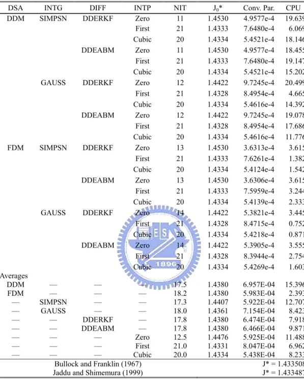
Table 4.4 Performance comparison of various numerical schemes for the oscillator problem, case I...64
Table 4.5 Various dynamic constraint treatments for the oscillator problem, case III. ...65
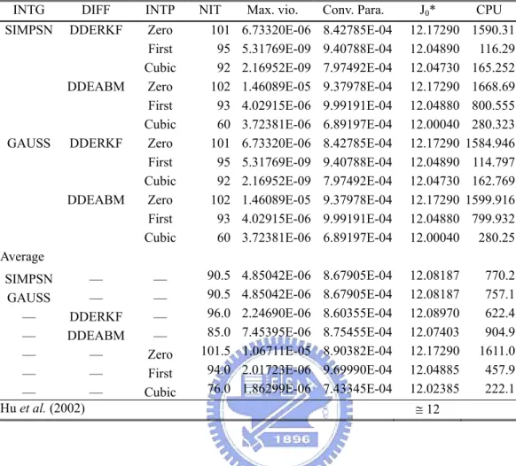
Table 4.6 Comparison of various numerical schemes for the overhead crane system. ...66
Table 5.1 Results of various methods for the F-8 fight aircraft problem. ...98
Table 5.2 Optimal results for the fourth-order system...99
Table 6.1 User subroutines for the flight level tracking problem...121
LIST OF FIGURES
Figure 2.1 Solution process based on indirect methods. ...21
Figure 2.2 Solution process based on direct methods. ...22
Figure 3.1 Methods for continuous constrained NLPs (Wu, 2000)...42
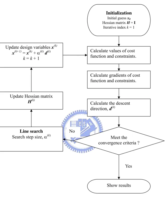
Figure 3.2 Conceptual flowchart of the SQP method...43
Figure 3.3 Problem-transcribing Process...44
Figure 3.4 Dynamic constraint treatments...45
Figure 3.5 Conceptual flowchart of the AOCP method...46
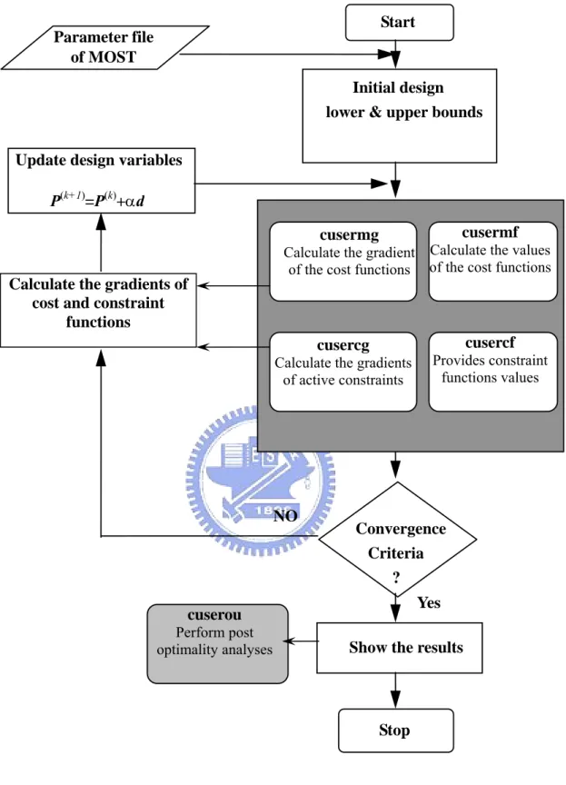
Figure 4.1 The architecture of MOST...67
Figure 4.2 Architecture of the interface coupler...68
Figure 4.3 Architecture of the new interface coupler – IAOS...69
Figure 4.4 Structure chart of the OCP Solver. ...70
Figure 4.5 CTRLMF module...71
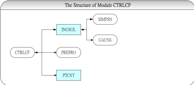
Figure 4.6 CTRLCF module...72
Figure 4.7 CTRMG module. ...73
Figure 4.8 CTRCG module. ...74
Figure 4.9 Connection architecture of MOST and OCP solver. ...75
Figure 4.10 User interfaces for MOST and the OCP solver. ...76
Figure 4.11 Flowchart for the OCP solver...77
Figure 4.12 Control and state trajectories for van de Pol oscillator problem, case I. ...78
Figure 4.13 Control and state trajectories for van de Pol oscillator problem, case II. ...79
Figure 4.14 Control and state trajectories of van de Pol oscillator problem, case III. ...80
Figure 4.15 Schematic of the overhead crane system (Hu et al., 2002)...81
Figure 4.16 State trajectories of the overhead crane system. ...82
Figure 4.17 Control trajectories for overhead crane system...83
Figure 4.18 State trajectories with different initial guess for overhead crane system...84
Figure 5.1 Conceptual layout of the branching process. ...100
Figure 5.2 Flow chart of the algorithm for solving discrete-valued optimal control problems. ...101
Figure 5.3 Control trajectories for the third-order system...102
Figure 5.4 State trajectories for the fourth-order system (Phase II). ...103
Figure 5.5 Control trajectories for the fourth-order system. ...104
Figure 5.7 Trajectories of the states and control input for the F-8 fighter aircraft. ...106
Figure 6.1 Aircraft model (Lygeros, 2003)...124
Figure 6.2 Numerical results for the tracking problem. ...125
Figure 6.3 Trajectories for the minimum time problem. ...126
Figure 6.4 Six-degrees-of-freedom vehicle model ...127
Figure 6.5 Sinusoidal displacement functions...128
Figure 6.6 Vehicle speed histories for straight-ahead accelerating. ...129
Figure 6.7 Vehicle speed histories for straight-ahead braking...130
Figure 6.8 Driver’s seat acceleration for straight-ahead braking. ...131
Figure 6.9 Road displacement profiles for model validation (Haug and Arora 1979). ...132
Figure 6.10 Road displacement profiles for emergency braking...133
Figure 6.11 Vehicle speed and acceleration histories for emergency braking...134
Figure 6.12 Seat acceleration and pitch angle histories for emergency braking. ...135
NOMENCLATURE
b design variablesd descent direction defined in SQP algorithm k iteration counter
s the wing surface area t0 start time
tf terminal time
u control variable vector
uc piecewise continuous control variable vector
ud discontinuous control variable vector
x state variable vector
BBk BFGS approximation of Hessian matrix CL dimensionless lift coefficient
CD dimensionless drag coefficient
D the aerodynamic drag force of a aircraft
H Hamiltonian function
HL Hessian matrix of the Lagrangian function
I interpolation function of control variables
Jmax Cost bound of mixed-integer NLP
J0 function of performance index (cost function) L the aerodynamic lift force of a aircraft
Lc (augmented) Lagrangian function N number of time intervals
Ns maximum iteration number of AOCP algorithm Ne number of equality constraints
NT number of inequality constraints
P extended design variable vector SD discretized control variable vector
S Parameter vector of interpolation function for controls T the thrust exerted by the aircraft engine
T time grid vector
Ti ith time grid point
U class of all such admissible controls
Ud class of all discontinuous admissible controls
α step size of SQP algorithm
ε convergence parameter of SQP algorithm
λ vector of Lagrange multipliers
( ) 1
l
ζ ith parameter of interpolation function for l time grid ρ the air density
Φi function of terminal state
Li integral part of performance index and functional constraints
CHAPTER 1
INTRODUCTION
1.1 Dynamic Optimization and Optimization Control Problems
Over the past decade, applications for dynamic systems in engineering have increased significantly. In most applications, the designs, which are based on a static model and obtained by traditional optimization methods, cannot work perfectly in dynamic cases because of their nonlinear behaviors. Therefore, researchers have devoted themselves to find an optimal design that is able to meet dynamic requirements.
Most engineering applications are modeled dynamically using differential algebraic equations (DAE) whose formulation consists of (a) differential equations that describe the dynamic behavior – such as mass and energy balances – of the state of a given system and (b) algebraic equations that ensure physical and dynamic relations. Usually, the dynamic behaviors of a given system can be influenced by the choice of certain control variables. For instance, a vehicle can be controlled by the steering wheel, the accelerator pedal, and the brakes. At the same time, the state and/or control variables cannot assume any value but are subject to certain restrictions, often resulting from safety regulations or physical limitations, such as the altitude of an aircraft being above ground level or the steering angle of a vehicle having a maximum limitation. In addition, engineers are particularly interested in those state and control variables that fulfill all restrictions while also minimizing or maximizing a given objective function. These problems are typically ones of dynamic optimization. By applying modeling and optimization technologies, a dynamic optimization problem can be reformulated as an optimal control problem (OCP).
Even though optimal control problems arise in various disciplines, not all engineers are familiar with optimal control theory. On the other hand, most optimal control problems are interpreted as an extension of nonlinear programming (NLP) problems to an infinite number of variables and solved by numerical methods. For engineers who are inexperienced in
numerical techniques, implementing these numerical techniques is another obstacle in solving dynamic optimization problems. Consequently, a general-purpose solver for optimal control problems coupled with a systematic procedure could assist engineers in solving various optimal control problems.
Time-optimal control problems (TOCP) have attracted the interest of researchers in optimal control because, even they often arise in practical applications, their solutions are difficult. In practical applications, one of the most common types of control function is the piecewise-constant function by which a sequence of constant inputs is used to control a given system with suitable switching times. Nevertheless, many methods proposed in the literature – for example, the switching time computations algorithm (Lucas and Kaya, 2001) – assume that the number of switching times is known before their algorithms are applied. In reality, however, the number of switching times is generally unknown before most control problems are solved. Therefore, an efficient algorithm for determining the switching times of TOCP becomes important and attracts the interest of researchers.
1.2 Literature Review
1.2.1 Methods for Optimal Control Problems
Optimal control problems can be solved by a variational method (Pontryagin et al., 1962) or by nonlinear programming approaches (Huang and Tseng, 2003, 2004; Hu et al., 2002; Jaddu and Shimemura, 1999). The variational or indirect method is based on the solution of first-order necessary conditions for optimality obtained from Pontryagin’s maximum principle (Pontryagin et al., 1962). For problems without inequality constraints, the optimality conditions can be formulated as a set of differential-algebraic equations, often in the form of a two-point boundary value problem (TPBVP). The TPBVP can be addressed using many approaches, including single shooting, multiple shooting, invariant embedding, or a discretization method such as collocation on finite elements. On the other hand, if the problem
requires that active inequality constraints be handled, finding the correct switching structure, as well as suitable initial guesses for the state and costate variables, is often very difficult.
Much attention has been paid in the literature to the development of numerical methods for solving optimal control problems (Hu et al., 2002; Pytlak, 1999; Jaddu and Shimemura, 1999; Teo, and Wu, 1984; Polak, 1971), the most popular approach in this field is the reduction of the original problem to a NLP problem. Nevertheless, in spite of extensive use of nonlinear programming methods to solve optimal control problems, engineers still spend much effort reformulating nonlinear programming problems for different control problems. Moreover, implementing the corresponding programs for the nonlinear programming problem is tedious and time consuming. Therefore, a general OCP solver coupled with a systematic computational procedure for various optimal control problems has become an imperative for engineers, particularly for those who are inexperienced in optimal control theory or numerical techniques.
Additionally, in many practical engineering applications, the control action is restricted to a set of discrete values. These systems can be classified as switched systems consisting of several subsystems and switching laws that orchestrate the active subsystem at each time instant. Optimal control problems for switched systems, which require solution of both the optimal switching sequences and the optimal continuous inputs, have recently drawn the attention of many researchers. The primary difficulty with these switched systems is that the range set of the control is discrete and hence not convex. Moreover, choosing the appropriate elements from the control set in an appropriate order is a nonlinear combinatorial optimization problem. In the context of time optimal control problems, as pointed out by Lee et al. (1997), serious numerical difficulties may arise in the process of identifying the exact switching points. Therefore, an efficient numerical method is still needed to determine the exact control switching times in many practical engineering problems.
1.2.2 Time-Optimal Control Problems
The TOCP is one of most common types of OCP, one in which only time is minimized and the control is bounded. In a TOCP, a TPBVP is usually derived by applying Pontryagin’s maximum principle (PMP). In general, time-optimal control solutions are difficult to obtain (Pinch, 1993) because, unless the system is of low order and is time invariant and linear, there is little hope of solving the TPBVP analytically (Kirk, 1970). Therefore, in recent research, many numerical techniques have been developed and adopted to solve time-optimal control problems.
One of the most common types of control function in time-optimal control problems is the piecewise-constant function by which a sequence of constant inputs is used to control a given system with suitable switching times. Additionally, when the control is bounded, a very commonly encountered type of piecewise-constant control is the bang-bang type, which switches between the upper and lower bounds of the control input. When the controls are assumed to be of the bang-bang type, the time-optimal control problem becomes one of determining the switching times, several methods for which have been studied extensively in the literature (see, e.g., Kaya and Noakes, 1996; Bertrand and Epenoy, 2002; Simakov et al., 2002). However, as already mentioned, in contrast to practical reality, these methods require that the number of switching times be known before their algorithms can be applied. To overcome the numerical difficulties arising during the process of finding the exact switching points, Lee et al. (1997) proposed the control parameterization enhancing transform (CPET), which they also extended to handle the optimal discrete-valued control problems (Lee et al., 1999) and applied to solve the sensor-scheduling problem (Lee et al., 2001).
In similar manner, this dissertation focuses on developing a numerical method to solve time-optimal control problems. This method consists of the two-phase scheme: first, switching times are calculated using existing optimal control methods; and second, the
resulting information is used to compute the discrete-valued control strategy. The proposed algorithm, which integrates the admissible optimal control problem formulation with an enhanced branch-and-bound method (Tseng et al., 1995), is then implemented and applied to some examples.
1.3 Objectives
The major purpose of this dissertation is to develop a computational method to solve the time-optimal control problems and find the corresponding discrete-valued optimal control laws. The other purpose of this dissertation is to implement a general OCP solver and provide a systematic procedure for solving OCPs that provides engineers with a systematic and efficient procedure to solve their optimal control problems.
1.4 Outlines
The dissertation is organized as follows. Chapter 2 introduces the formulations for various optimal control problems and the general methods for solving such problems. Also briefly discussed are problem-solving procedures and the difficulties with direct and indirect methods. Chapter 3 specifically addresses the computational methods for solving optimal control problems and presents the theoretical basis and numerical preliminaries for developing a general optimal control problem solver. The architecture of the OCP solver and the systematic procedure for solving the OCP are described in Chapter 4, which also present the details of the implementation and user interface of the proposed solver. Here, the van der Pol oscillator problem with various types of terminal conditions and the time-optimal control problem of overhead crane control are used to demonstrate and verify the capability and accuracy of the proposed OCP solver. Chapter 5 introduces a two-phase scheme that integrates the admissible optimal control problem method and the enhanced branch-and-bound algorithm to efficiently solve the bang-bang control problems in the field of engineering. In Chapter 6, the proposed
solver is applied to two practical engineering applications: the flight level control problem and the vehicle suspension design problem. Finally, Chapter 7 draws some conclusions and makes suggestions for further research.
CHAPTER 2
METHODS FOR SOLVING OPTIMAL CONTROL PROBLEMS
2.1
Introduction
Optimal control theory has been of considerable importance in a wide variety of disciplines. Over the years, the theory has been developed for various applications in many different fields, e.g., mechanical systems (Kim and Ha, 2001), automotive vehicle design (Panagiotis, 2000; Jalili and Esmailzadeh, 2001), and manufacturing processes (Samaras and Simaan, 2001). However, because most real-world problems are becoming too complex to be solved analytically (Kirk, 1970), using computational algorithms to solve them is becoming inevitable. As a result, several successful families of algorithms are now available in the literature.
Techniques for the numerical solution of optimal control problems can be broadly divided into direct and indirect methods (Bock, 1978; Stryk and Bulirsch, 1992). In the direct method, the state and/or control variables are parameterized using a piecewise polynomial approximation. Inserting these approximations into the cost functional, dynamic equations, and constraints and boundary conditions leads to a static parameter optimization problem. On the other hand, the indirect method is based on the solution of the first-order necessary conditions for optimality obtained from Pontryagin’s maximum principle (Pontryagin et al., 1962) or derived from the Hamilton-Jacobi-Bellman equation (Bellman, 1957).
Two early methods commonly used to solve optimal control problems are Bellman’s dynamic programming (Bellman, 1957) and Pontryagin’s maximum principle (Pontryagin et al., 1962). Dynamic programming, developed by Bellman in the late 1950s (Bellman, 1957; Bellman and Dreyfus, 1962; Bellman and Kalaba, 1965), is a computational technique that extends the decision-making concept to sequences of decisions, which together define an optimal policy and trajectory. Subsequently, Soviet mathematician Pontryagin and his
colleagues (Pontryagin et al., 1962) developed the calculus of variations approach using a maximum principle. Although both the dynamic programming method and PMP have been used to solve optimal control problems, many practical problems described by strongly nonlinear differential equations cannot be easily solved by either technique. As a result, many approximation methods based on NLP methods are used to solve these practical problems (see, e.g., Lin, 1992; Pytlak, 1999; Jaddu and Shimemura, 1999; Hu et al., 2002).
A nonlinear programming problem consists of a multivariable function subject to multiple inequality and equality constraints. The solution to the nonlinear programming problem is found by solving the Kuhn-Tucker points of equalities given by the first-order boundary conditions. Conceptually, this procedure is analogous to solving optimal control problems using Pontryagin’s maximum principle. Depending on the discretization technique applied, methods that apply NLP solvers can be classified into two groups: simultaneous or sequential strategies. In the simultaneous methods, the state and control variables are fully discretized and thus usually lead to large-scale NLP problems that require special solution strategies (Cervantes and Biegler, 1998; Betts and Huffman, 1992). However, in sequential methods – also known as control variable parameterization methods – only the control variables are discretized. Based on initial conditions and a set of control parameters, the system equations are integrated with an ordinary differential equation (ODE) solver at each iteration to produce cost functional (performance index) and constraint values used by a nonlinear programming solver to find the control parameterization’s optimal coefficient values. The sequential approach is a feasible path method, i.e., in each of iteration, the system equation is solved. However, this procedure is robust only when the system contains stable modes. Otherwise, finding a feasible solution for a given set of control parameters may be difficult. In this dissertation, a different discretization technique – the shooting method – is implemented and used in conjunction with sequential quadratic programming (SQP) to solve various types of
optimal control problems.
The shooting method serves as a bridge between sequential and simultaneous approaches by partitioning the time domain into smaller time intervals and integrating the system equations separately in each interval. Control variables are treated in the same manner as in the sequential approach. Moreover, to obtain gradient information, sensitivities are obtained for both the control variables and the initial state conditions in each time interval. Finally, equality constraints are added to the nonlinear program in order to link the time intervals and ensure that the states are continuous across each time interval. This method allows inequality constraints for both the state and the controls to be imposed directly at the grid points. Thus, the admissible optimal control problem (AOCP) formulation based on the shooting method is adopted as the core of the proposed method.
2.2 Canonical Formulation of Optimal Control Problems
Considering a dynamical system described by the following nonlinear differential equations on [0, tf ]:
(
t
, , ( ), ( ) ,
t
t
)
=
x
f
b x
u
t
∈ ⎣
⎡
0,
t
f⎤
⎦
(2.1)with the initial condition
0
(0)=
x x , (2.2)
where tf is the terminal time, b \∈ π is the vector of design variables,
[
]
T1 2
( ) ( ), ( ), , ( ) m m
t ≡ u t u t u t
u " ∈ \ is a vector of the control functions and
[
]
T 1 2 ( ) ( ), ( ), , ( ) n n t ≡ x t x t x t x " ∈ \ nis a vector of the state variables. The function is assumed to be continuously differentiable with respect to all its arguments, and is a given vector in . It is assumed that the process starts from t
: × π× n× m
f \ \ \ \ 6 \
0
x \n
0 = 0 and ends at the fixed terminal time tf > 0. A process that starts from t0 ≠ 0 may be transformed to satisfy this assumption by suitable shifting on the time axis. Let U be the class of all such
admissible controls. Then an optimal control problem may be stated formally as follows: Given the dynamical system expressed in Eqs. (2.1) and (2.2), find u ∈ U such that the cost
functional (performance index)
(
)
(
)
0 0 , ( ), 0 0 , ( ), ( ), f t f f J = Φ b x t t +∫
L b u t x t t dt (2.3)is minimized subject to the constraint
(
, ( ),)
0(
, ( ), ( ),)
0; 1,..., 0; 1,...., f t e i i f f i e T i N J t t t t t dt i N N = = ⎧ = Φ + ⎨≤ = + ⎩∫
b x L b u x (2.4)and the following continuous inequality constraint on the function of the state and control:
(
, ( ), ( ),)
0; 1,...,j t t t j q
ψ
b u x ≤ = ,∀ ∈ ⎣
t
⎡
0,
t
f⎤
⎦
. (2.5)where Φ0, L0, Φi, Li and ψjare continuously differentiable with respect to their respective
arguments. This problem is referred to as problem (PU). A control u ∈ U is said to be a
feasible control if it satisfies constraints (2.4) and (2.5).
The preceding definition extends the original Bolza problem to account for inequality constraints because the original Bolza formulation, containing only equality constraints, is not general for the OCP. It also fails to treat the design variables b, which may serve a variety of useful purposes apart from the obvious design parameters, e.g., weight and velocity of a vehicle. Moreover, when the terminal time tf is unconstrained (for optimization), a free-time
problem occurs. Otherwise, a fixed-time problem is given. In addition, the initial conditions are separated from the functional constraints in Eq. (2.4) for practical considerations, and the terminal conditions are treated as equality constraints in the first term of Eq. (2.4). The differential equations for the system in Eq. (2.1) are written in general first-order form. Equation (2.5) represents the mixed state and control inequality dynamic constraints.
According to the constraints encountered in practical applications, most constraints can be classified under one of the following categories (Teo et al., 1991):
Type 1. Control bounds:
min ≤ ( )t ≤ max
u u u ,
∀ ∈ ⎣
t
⎡
0,
t
f⎤
⎦
(2.6)Type 2. Terminal state constraint with fixed terminal time:
(
, ( ),)
0; 1,..., 0; 1,...., e i f f e T i N t t i N N = = ⎧ Φ ⎨≤ = + ⎩ b x , tf is fixed. (2.7)Type 3. Terminal state constraint with free terminal time:
(
, ( ),)
0i tf tf
Φ b x =
=
, tf is unspecified. (2.8)
Type 4. Interior point state constraint:
(
, ( ),)
0i t tl l
Φ b x ,0 < tl < tf (2.9)
Type 5. Integral constraint:
(
)
0 0; 1,..., , ( ), ( ), 0; 1,...., f t e i e T i N t t t dt i N N = = ⎧ ⎨≤ = + ⎩∫
L b u x (2.10)Type 6. Continuous equality constraint on the function of the state and control:
(
, ( ), ( ),)
0i t t t
Φ b x u = ,
∀ ∈ ⎣
t
⎡
0,
t
f⎤
⎦
(2.11)Type 7. Continuous inequality constraint on the function of the state and control:
(
, ( ), ( ),)
0i t t t
Φ b x u ≤ ,
∀ ∈ ⎣
t
⎡
0,
t
f⎤
⎦
(2.12)To develop a general optimal control solver, any constraint of type 2 to type 7 can be regarded as a special case of Eqs. (2.4) and (2.5).
2.3 First-Order Necessary Condition – Euler Lagrangian Equation
The first-order necessary condition for optimality, known as the Euler-Lagrangian equation, can be found in many research studies (e.g., Teo et al., 1991; Kirk, 1970). Given an optimal control problem where control u ∈ U is chosen such that the cost functional defined
(
)
(
)
0 0 ( ), 0 0 ( ), ( ), f t f f J = Φ x t t +∫
L u t x t t dt (2.13)where Φ0 and L0 are continuously differentiable with respect to their respective arguments. It should be noted that the cost functional may be regarded as depending explicitly only on u, as x is implicitly determined by u from Eqs. (2.1) and (2.2). In addition, the design variables vector, b, is treated as a constant and is not involved. The system equations (2.1) and (2.2) can be appended to the cost functional by introducing the appropriate Lagrange multiplierλ∈ \n:
( )
(
( )
)
{
(
( ) ( )
)
( )
( )
(
( ) ( )
)
( )
}
0 0 0 0 f t f f T J t t t t t t t t t t = Φ + dt ⎡ ⎤ + ⎣ − ⎦∫
u x , , x ,u λ f , x ,u x L (2.14)The Hamiltonian function is defined as follows:
(
)
0(
)
(
)
H , x,u, λt = t, x,u +λ f , x,uT t
L (2.15)
It should again be noted that, if the system equation is satisfied, the appended cost functional J is indifferent to the original0 . The time dependent Lagrange multiplier is referred to as the costate vector, also known as the adjoint vector.
0
J
Substituting Eq. (2.15) into Eq. (2.14) and integrating the last term by parts, the cost functional becomes
( )
(
( )
)
(
( )
)
( )
(
( )
)
( )
( ) ( ) ( )
(
)
{
( )
( )
( )
}
0 0 0 0 0 u x λ x λ x H , x ,u , λ λ x f T T f f f T t J t t t t t t t t t d = Φ − + +∫
+ t (2.16)For a small variation c in u, the corresponding first-order variations in x and J are 0 δx
( )
(
( )
)
(
( )
)
( )
(
( )
)
( )
( ) ( ) ( )
(
)
( )
( )
( )
( ) ( ) ( )
(
)
( )
0 0 0 0 0 x u λ x λ x x H , x ,u , λ λ x x H , x ,u , λ u u f T T f f T t t J t t t t t t t t t t t t dtδ
δ
δ
δ
⎡∂Φ ⎤ =⎢ − ⎥ + ∂ ⎢ ⎥ ⎣ ⎦ ⎧⎡∂ ⎤ ⎪ + ⎨⎢ ∂ + ⎥ ⎢ ⎥ ⎪⎣ ⎦ ⎩ ⎫ ∂ ⎪ + ⎬ ∂ ⎪⎭∫
tδ
(2.17)Since λ t
( )
is arbitrary so far, it can be set as( )
( )
λ H , x(
( ) ( ) ( )
,u , λ)
x T t t t t t = −∂ ∂ (2.18)with boundary condition:
( )
(
)
0(
x( )
)
λ x T f f t t =∂Φ ∂ (2.19)As the initial condition x(0) is fixed, δx
( )
0 vanishes and Eq. (2.17) reduces to( )
(
( ) ( ) ( )
)
( )
0 0 * H , x ,u , λ u u u f t t t t t J tδ
= ⎧⎪⎨∂δ
⎫⎪⎬dt ∂ ⎪ ⎪ ⎭ ⎩∫
(2.20)For a local minimum, it is necessary that δJ0 vanishes for arbitraryδx. Therefore, it is necessary that
( ) ( ) ( )
(
)
0
H , x
,u
, λ
u
t
t
t
t
∂
=
∂
(2.21)for all t∈ ⎣⎡0,tf⎤⎦ , except on a finite set. It should be noted that this holds only if no bounds on u exist; otherwise, the Pontryagin’s maximum principle to be discussed later will be
applied. Equations (2.1), (2.2), (2.18), (2.19), and (2.21) are the well-known Euler-Lagrangian equations whose results can be summarized in the following theorem.
Theorem 2.1 If u*(t) is a control that yields a local minimum for the cost functional (2.13), and x*(t) and λ*(t) are the corresponding state and costate, then it is necessary that
( )
(
x t)
(
( ) ( ) ( )
)
= f t(
, x*( ) ( ) ( )
t ,u* t , λ* t)
( )
(
)
(
( ) ( ) ( )
)
* * * * T T ⎡∂ t t t t ⎤ ⎢ ⎥ = ∂ ⎢ ⎥ ⎣ ⎦ H , x ,u , λ λ (2.22a)( )
* 00
=
x
x
(2.22b) * * * * T t t t t t = −⎡⎢∂ ⎤⎥ ∂ ⎢ ⎥ ⎣ ⎦ H , x ,u , λ λ x (2.22c)( )
0(
*( )
)
T f f t t ⎡∂Φ ⎤ ⎢ ⎥ = ⎢ ∂ ⎥ ⎣ ⎦ x λ x 0, (2.22d)and, for all t∈ ⎣⎡ tf⎦⎤, except possibly on a finite subset of ⎡⎣0, tf⎤⎦
( )
,( ) ( )
(
)
0
H , x
,u
, λ
u
t
t
t
t
∂
=
∂
(2.22e)It should be noted that Eqs. (2.22a)-(2.22d) constitute 2n differential equations with n boundary conditions for x* specified at t = 0 and n boundary conditions for λ* specified at t = tf. This is referred to as a two-point boundary value problem. In principle, the dependence
on u* can be removed by solving u* as a function of x* andλ* from the m algebraic equations in Eq. (2.22e) via the implicit function theorem, provided that the Hessian
H H u u T uu ∂ ∂⎡ ⎤ ≡ ⎢ ⎥
∂ ⎣∂ ⎦ is nonsingular at the optimal point.
2.4 Methods for Solving Optimal Control Problems 2.4.1 Indirect Methods
As mentioned in Section 1.2.1, the indirect method is based on the solution of the first-order necessary conditions for optimality obtained from Pontryagin’s maximum principle (Pontryagin et al., 1962), which has been modified and applied in various applications (see,
e.g., Xu and Antsaklis, 2004; Chyba et al.,2003; Steindl and Troger, 2003). For problems without inequality constraints, the optimality conditions can be formulated as a set of differential-algebraic equations (DAEs). Obtaining a solution to DAEs requires careful attention to the boundary conditions because the state variables frequently have specified initial conditions and costate (adjoint) variables whose final conditions result in a TPBVP that is notoriously difficult to solve analytically and requires the use of iterative numerical techniques (Kirk, 1970). On the other hand, if the problem requires that active inequality constraints be handled, finding the correct switching structure together with suitable initial guesses for state and costate variables is often very difficult because of a lack of physical significance and the need for prior knowledge of the control’s switching structure. Many numerical techniques, including single shooting, invariant embedding, and multiple shooting, can be used to solve TPBVP, but PMP does not deal well with nonlinear optimal control problems. Figure 2.1 shows a solution process based on indirect methods.
Pontryagin’s Maximum Principle
According to the Euler-Lagrangian equation for the unconstrained optimal control problem of Section 2.3 depicts that the Hamiltonian function must necessarily be
stationary with respect to the control, i.e. H 0
u
∂ =
∂ at optimality. However, the optimality condition obtained in Section 2.3 does not have to be satisfied if the control is constrained to lie on the boundary of a subset Us. Here, Us is a compact subset of . Then, the Pontryagin’s maximum principle can be described by the following theorem:
r
\
Theorem 2.2 Given the problem, where the cost functional (2.13) is to be minimized over U subjected to the system equations (2.1) and (2.2), if u*(t) ∈ U is an optimal control, and x*(t) and λ*(t) are the corresponding state and costate, then it is necessary that
( )
(
*)
(
*( ) ( ) ( )
* *)
(
*( ) ( ) ( )
* *)
T t t t t t =⎡⎢∂ ⎤⎥ = f t t t t ∂ ⎢ ⎥ ⎣ ⎦ H , x ,u , λ x , x ,u , λ λ( )
* 00
=
x
x
( ) ( )
(
)
T (2.23a) (2.23b)( )
(
)
*( )
* * T t t ⎡ ⎤ ⎢ ⎥ ⎢ ⎥ ⎣ ⎦ ,u , λ x( )
* t = − ∂ t t ∂ H , x λ (2.23c)( )
(
*)
0 f T t t ⎡∂Φ ⎤ ⎢ ⎥ = x λ 0, f ⎢ ∂ ⎥ ⎣ x ⎦ (2.23d)and, for all t∈⎣⎡ tf⎦⎤, except possibly on a finite subset of ⎡⎣0, tf⎤⎦
( )
,( ) ( )
(
t
*t
*t
*t
)
≤
(
t
*( ) ( ) ( )
t
t
*t
)
H , x
,u
, λ
H , x
,u
, λ
(2.23e) for all t∈ ⎣⎡0,tf⎤⎦ . Dynamic ProgrammingDynamic programming (DP), based on Bellman’s principle of optimality (Bryson and Ho, 1975; Bellman and Dreyfus, 1962; Bellman, 1957), requires solution of the Hamilton-Jacobi-Bellman partial differential equation in a domain of the state space that contains the optimal solution. In dynamic programming, the optimal control problem is expressed as a state-variable feedback in graphical or tabular form. Optimal control strategies must be determined by working backward from the final stages. In other words, this method operates in sweeps through the state set, performing a full backup operation on each state. Each backup updates the value of one state based on the value of all possible successor states. The computational procedure for dynamic programming can be described briefly by the following steps.
In this step, the time interval, [t0, tf], is divided into N equal spaced intervals, Δt, and
the performance index and state equations are converted into discrete form. Then, by applying the principle of optimality, the performance index can be converted into recurrent form:
(
)
(
)
( ){
(
)
* , D * ( 1), min , ( ), ( ) ( ( , ( ), ( )))} N k N u N k N k N N k N k N k t N k N k − − − − − = − − + Δ ⋅ − − J x b u x J f b x u L (2.24) Step 2: Quantizing the admissible state and control values into a finite number of levels. Step 3: Calculating and storing the minimum values of the performance index of each stagefrom final state to initial state. In each stage, every quantized control value is tried at each quantized state value to discover the corresponding state values of the next stage. Additionally, the value of the performance index from current stage to final stage is calculated and compared. The minimum performance index is then chosen and stored. If the corresponding state values of the next stage are not in the quantized grid points, interpolation is required.
Step 4: Showing the results.
2.4.2 Direct Methods
Direct methods try to solve the dynamic optimization problem directly without explicitly solving the necessary conditions. Usually, these methods are based on an iterative procedure that generates approximations to the optimal solution of the dynamic optimization problem within each iteration step. For instance, the SQP method uses quadratic subproblems to approximate a general nonlinear programming problem locally.
As mentioned in Section 2.1, most direct methods that apply NLP solvers can be classified into simultaneous and sequential strategies. The important question for these numerical direct methods is whether these iterative approximate algorithms converge to a solution of the original problem or not. A solution process based on such methods is shown in Figure 2.2 and
their details will be introduced in Chapter 3.
2.5 Summary
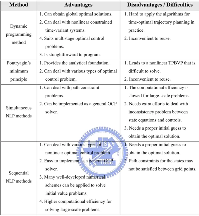
The primary objective of this chapter has been to survey methods of the optimal control problems and provide formulations of various types of optimal control problems. The first-order necessary condition (Euler-Lagrangian equation) has also been briefly introduced to provide the theoretical foundation for Pontryagin’s maximum principle. In addition, the chapter has described two typical methods for solving optimal control problems – indirect and direct approaches – whose advantages and drawbacks are listed in Table 2.1. Understanding the advantages of and difficulties with these methods will help engineers apply them to problem solving.
As regards applicability, dynamic programming (DP) is sometimes thought to be limited because of “the curse of dimensionality” (Bellman, 1957), i.e., the fact that the number of states often grows exponentially with the number of state variables. In reality, even though large state sets do create difficulties, these are the inherent difficulties of the problem not of DP as a solution method. In fact, the DP method can be used with today’s computers to solve optimal control problems with millions of states. In particular, dynamic programming can deal with multistage optimal control problems that are difficult to solve using other methods. Nevertheless, even though dynamic programming can be used to solve optimal control problems in nonlinear time-variant systems, using it to deal with time-optimal trajectory planning is difficult in practice because it relies on the exact dynamic models of the system. Yet, unfortunately, the time-optimal control problem is a very common application of the optimal control problem.
In contrast, Pontryagin’s maximum principle, which provides the analytical foundation for this study, can deal with various types of optimal control problem. However, in any such control problem, PMP unfortunately leads to a nonlinear two-point boundary value problem
that, as earlier mentioned, is notoriously difficult to solve analytically and requires the use of iterative numerical techniques (Kirk, 1970).
Furthermore, neither DP nor PMP can serve as a convenient and complete method for reformulating different control problems. Rather, engineers either have to derive the state equations, costate equations, and boundary conditions from PMP or have to reformulate the discrete form of the system equations and performance index by applying the DP algorithm. Engineers must then also implement numerical programs to solve the TPBVP using PMP or execute recurrence equations using DP. For engineers inexperienced in optimal control theory or numerical techniques, carrying out these theoretical derivations and program implementations is difficult. Thus, a general-purpose solver is needed for various types of optimal control problems.
From a practical viewpoint, of the two types of NLP methods compared in Section 2.1 (simultaneous and sequential strategies), the sequential NLP methods are the best for developing a general-purpose problem solver.
Table 2.1 Comparison of the methods for solving optimal control problems.
Method Advantages Disadvantages / Difficulties
Dynamic programming
method
1. Can obtain global optimal solutions. 2. Can deal with nonlinear constrained
time-variant systems.
4. Suits multistage optimal control problems.
3. Is straightforward to program.
1. Hard to apply the algorithms for time-optimal trajectory planning in practice.
2. Inconvenient to reuse.
Pontryagin’s minimum
principle
1. Provides the analytical foundation. 2. Can deal with various types of optimal
control problem.
1. Leads to a nonlinear TPBVP that is difficult to solve.
2. Inconvenient to reuse.
Simultaneous NLP methods
1. Can deal with path constraint problems.
2. Can be implemented as a general OCP solver.
1. The computational efficiency is slowed for large-scale problems. 2. Needs extra efforts to deal with
inconsistency problem between state equations and controls. 3. Needs a proper initial guess to
obtain the optimal solution.
Sequential NLP methods
1. Can deal with various types of nonlinear optimal control problem. 2. Easy to implement as a general OCP
solver.
3. Many well-developed numerical schemes can be applied to solve initial value problems.
4. Higher computational efficiency for solving large-scale problems.
1. Needs a proper initial guess to obtain the optimal solution. 2. Path constraints for the states may
Dynamic Optimization Problem Necessary Conditions Complementarity Problem Algorithm Candidate
Check for optimality (sufficient conditions)
Dynamic Optimization Problem
Iterative / approximative Algorithm (SQP)
Solution
Check for convergence or optimality (sufficient / necessary conditions)
CHAPTER 3
COMPUTATIONAL METHODS AND NUMERICAL PRELIMINARIES
FOR SOLVING OCP
3.1 Introduction
The rapid advancements in modern computers have brought about a revolution in the solutions to many physical and engineering problems, including optimal control problems. However, most real-world problems are becoming too complex to allow analytical solution; thus, computational methods must inevitably be used in solving them. As a result, computational methodology has attracted the interest of many engineers and mathematicians, and over the last two decades, many state-of-the-art computational methods for optimal control theory – including collocation transcription and the AOCP method – have been developed (see, e.g., Betts, 1998 and 2001; Hu et al., 2002; Jaddu and Shimemura, 1999; Lin, 1992; Pytlak, 1999).
Some earlier computational methods for solving optimal control problems were based on the indirect approach that assumes the direct solution of a set of necessary optimality conditions resulting from Pontryagin’s maximum principle. The adjoint (co-state) equations are combined with the original state equations to form a TPBVP. This problem may be efficiently solved using the shooting method discussed earlier, which guesses the unknown initial values of the adjoint variables, integrates both system and adjoint equations forward, and then reestimates the initial guesses from residuals at the end point (Bulirsch, 1971; Lastman, 1978). Nevertheless, because of difficulties arising from the sensitivity and instability of the solutions to the initial guesses, Bulirsch and his coworkers (1971, 1980) introduced multiple shooting algorithms to improve convergence and stability. Multiple shooting refers to the breaking up of a trajectory into subintervals, on each of which an initial-value problem is defined. The solutions are then adjusted in successive iterations until the boundary conditions and continuity properties at the ends of the subintervals are satisfied.
Multiple shooting is much more successful than its ancestor, the simple shooting method, in which a single initial-value problem is defined. However, even though especially good convergence properties are attributed to multiple-shooting algorithms, the necessity to define the proper control structure and initialize the adjoint variables within a sufficient vicinity of the optimal values still remains a serious limitation.
To avoid the drawbacks of shooting techniques, the direct methods have been studied extensively during the last two decades (Betts, 1993; Barclay, 1997; Gill et al., 2002). One of the most widely used methods for solving optimal control problems is the direct method whose basis is the transformation of the optimal control problem into a NLP problem using either the discretization or parameterization technique (see, e.g., Goh and Teo, 1988; Xu and Antsaklis, 2004; Jaddu, 2002; Lee et al., 1999).
When the discretization technique is applied, the optimal control problem is converted into a nonlinear programming problem with a large number of unknown parameters and constraints (Betts, 1998). On the other hand, parameterizing the control variables (Goh and Teo, 1988; Teo et al., 1991) requires integration of the system equations. Moreover, the simultaneous parameterization of both the state variables and the control variables also results in a nonlinear programming problem with a large number of parameters and equality constraints.
As a prelude to discussing computational methods for solving optimal control problems, the following sections introduce some fundamental NLP concepts. Also introduced is one of the best and most frequently applied NLP methods for solving optimal control problems, sequential quadratic programming (see Barclay, et al., 1998; Betts, 2000; Gill et al., 2002; Kraft, 1994; Stryk, 1993). Subsequently, the AOCP method, which uses the discretization technique to convert an OCP into a NLP problem, is proposed, and then a standard SQP algorithm is applied to solve it. Also discussed are the dynamic constraint treatments and
design sensitivity analysis used in AOCP.
3.2 Nonlinear Programming Problem
Mathematically, the general form of a constrained NLP problem can be expressed as follows: minimize f(x) subject to g(x) ≤ 0 , xT = (x 1, …, xn) h(x) = 0 (3.1)
where f(x) is the objective function, and h(x) and g(x) are the equality and inequality constraint functions, respectively. It should be noted that in the inequality constraint functions
g(x), the simple bounds of the design variables (xL ≤ x ≤ xU) are considered and classified.
Because maximization problems can be converted to minimization ones by negating their objectives, only minimization problems are considered here, without loss of generality.
A general continuous constrained NLP problem is defined in Eq. (3.1) in which x is a vector of continuous variables. Over the past three decades, a variety of methods has been produced in a wide body of research to solve the general constrained continuous optimization problem (Betts, 2001; Michalewicz et al., 1996; Horst and Tuy, 1993; Floudas and Pardalos, 1992; Hansen, 1992). Based on different problem formulations, existing methods can be classified into three categories: penalty formulations, direct solutions, and Lagrangian methods. Figure 3.1 classifies these methods according to their formulations, and the details of these methods and their comparisons can be found in Wu (2000). Here, the SQP method based on the Lagrangian method and adopted as an NLP solver in the AOCP algorithm is introduced briefly.
constraints are first transformed into their equal equivalents before Lagrangian methods are applied. For example, an inequality constraint can be transformed into an equality constraint by adding a slack variable (Luenberger, 1984). Thus, a general continuous equality constrained optimization problem can be formulated as follows:
minimize f(x)
subject to
h(x) = [h1(x), …, hm] T = 0
(3.2)
where xT = (x1, …, xn) is a vector of the continuous variables. Both f(x) and h(x) are assumed to be continuous functions that are at least first-order differentiable. The augmented Lagrangian function in continuous space in Eq. (3.2) is then defined as
( )
( )
( )
1( )
22
Lc x λ, ≡ ∇xf x + ∇λT xh x + h x (3.3)
where λ is a vector of the Lagrange multipliers. Compared to the conventional Lagrangian function in continuous space defined as
(
)
( )
T(
c x λ ≡ f x +λ h x
L ,
)
, the augmentedLagrangian function reduces the possibility of ill conditioning and is, therefore, more stable. Various continuous Lagrangian methods have been developed to find the (local) optimum, all based on first-order necessary conditions. To state these conditions, the concept of regular points must first be introduced.
Definition 3.1. A point x, which satisfies constraints h(x) = 0, is said to be a regular point (Luenberger, 1984) if the gradient vectors ∇h1
( )
x ,∇h2( )
x ,…,∇hm( )
x at point x are linearly independent.First-order necessary conditions for continuous constrained NLP problems.
Letting x be a (local) optimal solution of f(x) subject to constraints h(x) = 0, and assuming that x is a regular point, then there exists λ \∈ msuch that