利用漸近邊界條件分析表面波於皺褶結構之色散

國

立

交

通

大

學

電信工程研究所

碩 士 論 文

利用漸近邊界條件分析表面波於皺褶結構之色散

Surface Wave Dispersion Analysis of Planar Corrugated

Surfaces by Asymptotic Corrugations Boundary Conditions

研 究 生：嚴大龍 (Ta-Lung Yen)

指導教授：黃謀勤 博士 (Dr. Malcolm Ng Mou Kehn)

i

利用漸近邊界條件分析表面波於皺褶結構之色散

學生：嚴大龍

指導教授

：

黃謀勤 博士

國立交通大學電信工程研究所碩士班

摘

要

電磁能隙(Electromagnetic Bandgap, EBG)結構在近年來被廣泛的研究

與 應 用 ， 而 皺 褶 性 結 構 是 其 代 表 之 一 。 在 探 討 EBG 結 構 時 ， 色 散 圖

(Dispersion diagram)和反射相位(Reflection phase)是兩個最重要的特

性。在此篇論文中，我們將研究如何準確及快速地獲得皺褶性結構的色散

圖，藉由近似法和邊界條件，從基本向量勢與電磁場的關係中推導出其特

徵方程式，從方程式進而得到完整的色散圖。接著我們會與傳統獲取色散

圖的方法: 橫向共振技術 (Transverse Resonance Technique, TRT)以及

模擬軟體來做比較，藉此來評估其準確性及快速性。我們最後也實際建造

了一個皺褶性結構，藉由散射參數來間接證明此特徵方程式所得的色散

圖。

傳統上研究皺褶性結構時，會著重當波行進方向為在皺褶結構表面上 0

度或者 90 度時的情況，也就是所謂的軟和硬表面(Soft/Hard surfaces)。

此篇論文會進一步探討波斜向入射時的情況。藉由觀察皺褶性結構的色散

圖，我們將會發現其與一般週期性結構不一樣的地方，故我們亦會研究此

特性對於不同方向的表面波在皺褶性結構上行進時會有何影響。

在量測階段時，通常無法直接獲取色散圖，而必須透過散射參數來間接

說明，然而我們希望能夠透過量測還原出色散圖。因此在此篇論文，我們

探討散射參數與波數之間的關係，期許可以將量測的散射參數有效地還原

成色散圖。目前我們已經可以將模擬的散射參數數據還原成色散圖，期許

將來可以應用在實際地量測數據。

-ii-

Surface wave dispersion analysis of planar corrugated surfaces by asymptotic

corrugations boundary conditions

Student：

嚴大龍

Advisor：Dr. Malcolm Ng Mou Kehn

Institute of Communications Engineering

National Chiao Tung University

ABSTRACT

Electromagnetic bandgap (EBG) structures had been widely investigated in

literature in recent years, and the planar corrugated surface is one of them. In

studying such structures, the dispersion and reflection phase diagrams are two of

the most important characteristics. In this thesis, we will study how to retrieve

the dispersion diagram of the corrugations accurately and rapidly. By an

asymptotic method and the use of classical vector potentials, we can derive the

characteristic equation, thereby obtaining the surface-wave dispersion diagram.

To demonstrate its accuracy and quickness, the method we proposed will be

compared to a full wave simulator and the transverse resonance technique (TRT),

the latter being a traditional method for getting the dispersion diagram. Finally,

we fabricated a corrugation, and measure its scattering parameters to indirectly

verify the dispersion diagram obtained by the method we proposed.

In traditional studies of corrugations, surface-wave propagations along only

the two principal directions are considered, pertaining to the so-called soft and

hard surfaces. In this thesis, we will further explore the situation whereby the

wave propagates obliquely on the surface. By observing the dispersion diagram

of the corrugations, we will notice its difference compared to normal periodic

structures, and then explain the wave propagation properties on the corrugation

surface.

At the measurement stage, it is difficult to get the dispersion diagram directly,

and usually the scattering parameters are used to explain the width and position

-iii-

in the frequency spectrum of the bandgaps. In the thesis, the relationship of the

scattering parameters and wavenumbers are discussed, so that the measured

scattering parameters can be transformed to the dispersion diagram effectively.

So far we succeed in transforming the simulated scattering parameters to the

dispersion diagram, and we hope this method can be applied to measured data in

the future.

-iv-

誌謝

首先感謝我的指導教授 黃謀勤博士在我碩士生涯這兩年的指導與栽

培，無論何時去他的辦公室請教問題，總是願意撥空來指導我，並且在研

究上給予我專業的知識以及正確的方向。也謝謝他給予我機會讓我參加國

外的會議論文研討，讓我見識到了來自各國學者精闢的報告，同時第一次

以英文演說也是一個難忘的經驗。

另外，我也要感謝我實驗室的同學樞彥，由於我們是 黃謀勤博士第一

屆的學生，在這兩年中樞彥幫忙處理了很多實驗室的事情，讓實驗室的運

作漸漸步上軌道。同時在研究的過程，我們也常常彼此互相討論交流，在

這過程讓我收穫良多。也謝謝光子晶體實驗室的正元、芳銚、和宜哲學長，

在我研究遇到瓶頸或者軟體操作上有問題時，都能適時給予寶貴的意見與

幫助。也謝謝實驗室的學弟妹:建融、博丞、怡嘉、以及 Lallah，你們的加

入讓實驗室的氣氛更熱鬧、更有活力。

最後，我要謝謝我的家人，在這兩年來的支持與鼓勵，他們從不給我

壓力，讓我每次回高雄時都覺得像充了一次電，回學校時更能專心在我的

研究上，你們的疼愛與關懷使我備感溫馨。

-v-

TABLE OF CONTENTS

CHINESE ABSTRACT

………

i

ENGLISH ABSTRACT

………

ii

ACKNOWLEDGEMENT ………

iv

TABLE OF CONTENTS ………

v

LIST OF FIGURES

………

vi

CHAPTER 1

Introduction………

1

CHAPTER 2

Theory………

4

2.1

Characteristic equation of the corrugation……

4

2.2

Refinement factor of the characteristic equation 11

2.3.1

An arbitrary example………

12

2.3.2

ACBC method compared to CST………

14

2.4

Influence of Refinement factor ………

17

2.5

ACBC method compared to TRT………

19

2.6

Field distributions………

22

CHAPTER 3

Sectorial bandgap………

25

3.1

Dispersion diagram corresponding to Brillouin

zone………

25

3.2

Concept of sectorial bandgap………

27

3.3

Sectorial bandgap corrugations design………

29

3.4

Simulation results………

33

3.5

Measurement results………

36

CHAPTER 4

Relationship between the scattering parameters

and dispersion diagram………

41

4.1

Introduction……… 41

4.2

Theory………

43

4.3

Verification ………

47

CHAPTER 5

Conclusion………

50

-vi-

LIST OF FIGURES

Figure 1

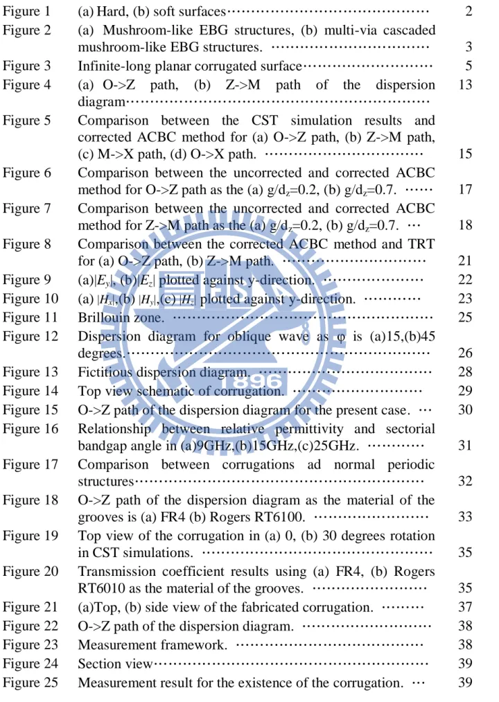
(a) Hard, (b) soft surfaces………

2

Figure 2

(a) Mushroom-like EBG structures, (b) multi-via cascaded

mushroom-like EBG structures. ………

3

Figure 3

Infinite-long planar corrugated surface………

5

Figure 4

(a) O->Z path, (b) Z->M path of the dispersion

diagram………

13

Figure 5

Comparison between the CST simulation results and

corrected ACBC method for (a) O->Z path, (b) Z->M path,

(c) M->X path, (d) O->X path. ………

15

Figure 6

Comparison between the uncorrected and corrected ACBC

method for O->Z path as the (a) g/d

z

=0.2, (b) g/d

z

=0.7. ……

17

Figure 7

Comparison between the uncorrected and corrected ACBC

method for Z->M path as the (a) g/d

z

=0.2, (b) g/d

z

=0.7. …

18

Figure 8

Comparison between the corrected ACBC method and TRT

for (a) O->Z path, (b) Z->M path. ………

21

Figure 9

(a)|E

y

|, (b)|E

z

| plotted against y-direction. ………

22

Figure 10

(a)

|Hx|

,(b)

|Hy|

,(c)

|Hz|

plotted against y-direction. …………

23

Figure 11

Brillouin zone. ………

25

Figure 12

Dispersion diagram for oblique wave as φ is (a)15,(b)45

degrees.………

26

Figure 13

Fictitious dispersion diagram. ………

28

Figure 14

Top view schematic of corrugation. ………

29

Figure 15

O->Z path of the dispersion diagram for the present case. …

30

Figure 16

Relationship between relative permittivity and sectorial

bandgap angle in (a)9GHz,(b)15GHz,(c)25GHz. …………

31

Figure 17

Comparison between corrugations ad normal periodic

structures………

32

Figure 18

O->Z path of the dispersion diagram as the material of the

grooves is (a) FR4 (b) Rogers RT6100. ………

33

Figure 19

Top view of the corrugation in (a) 0, (b) 30 degrees rotation

in CST simulations. ………

35

Figure 20

Transmission coefficient results using (a) FR4, (b) Rogers

RT6010 as the material of the grooves. ………

35

Figure 21

(a)Top, (b) side view of the fabricated corrugation. ………

37

Figure 22

O->Z path of the dispersion diagram. ………

38

Figure 23

Measurement framework. ………

38

Figure 24

Section view………

39

Figure 25

Measurement result for the existence of the corrugation. …

39

-vii-

Figure 26

Comparison for the results as the corrugation rotates 0

degree and 30 degrees. ………

40

Figure 27

Equivalent circuit model of an infinite long periodically

loaded transmission line. ………

42

Figure 28

Two port network. ………

44

Figure 29

Multi-reflections in the material. ………

44

Figure 30

Comparison between the new material and the corrugation

for S

21

. ………

47

Figure 31

Scattering parameters for the relative permittivity of the

grooves as (a) 10.2, (b) 6.15.………

48

Figure 32

Comparison between the corrected ACBC method and

retrieving method from scattering parameters as the relative

1

I. Introduction

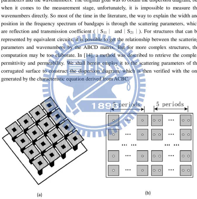
Corrugations have been an objective of keen interest in electromagnetic theory for many decades. Elliott was one of the earliest pioneers, who studied the surface wave propagation over a corrugated metallic ground plane, and has been concerned with the problem where the directions of wave propagation across the surface is normal to the corrugations [1]. Since the wave propagation direction will not always be normal to the corrugation, Hougardy and Hansen studied the surface wave propagation along an oblique angle with the orientation of the corrugations [2].

Theoreticians and computational enthusiasts were not the only ones captivated by this structure. Experimentalists and practical engineers have, likewise for the past many years, been making use of corrugations to develop improved microwave devices such as waveguides and antenna. The most known applications for corrugation are soft and hard surfaces, and the ideas were first introduced by Kildal [3] [4]. These surfaces triggered interests from enormous researchers because they can control the behavior of wave propagation over them. In other words, wave propagation can either be suppressed (soft) or enhanced (hard) on these surfaces, as shown in Fig.1. For examples, the soft surface is often called “chokes” and used to reduce the cross-polarization and sidelobes in particular directions. The hard surface is used to design hard horns which have high aperture efficiency or reduce scattering from masts that block the radiation field of an antenna [5].

The soft and hard surfaces have similar notions with the electromagnetic bandgap (EBG) structures, whereby both demonstrate the wave propagation existed in some frequency band and prohibited in others. In [6], the EBG structures are defined as artificial periodic objects that prevent/assist the propagation of electromagnetic waves in a specified band of frequency “for all incident angles” and all polarization states, while only for some specular angles for soft and hard surfaces. The EBG structures have become a popular topic in the antenna community since its useful application. The attracting features include designing an efficient low profile wire antenna near a ground plane [7], being applied for high gain resonator antennas [8], and for surface wave suppression [9]. Despite the numerous works on corrugated surfaces found in literature, none has studied them in terms of the dispersion diagram conveying the surface-wave passband and stop-band properties, or presented characteristic equations from which the aforementioned diagram is obtained. Field distributions of the surface wave modes supported by the corrugations are also nowhere to be found.

The main properties when investigating the periodic structures will be the dispersion diagram and reflection phase. In this thesis, we will focus on the points with the dispersion diagram of the corrugation. Due to the complexity of the EBG structures, it is usually difficult to characterize them by analytical methods. So we can utilize approximate boundary

2

conditions (ABC) to provide an approximate relationship between the electric and magnetic field on a chosen surface. The simplest case might be the first order impedance conditions, sometimes referred to as SIBC (Standard Impedance Boundary Conditions), which are applicable at the surface of a lossy dielectric. For some cases, the accuracy of SIBC is not sufficient, so generalized impedance boundary condition (GIBC) with more degrees of freedom is proposed to have higher accuracy. The works in [10] and [11] have used such approximate impedance boundary conditions to study corrugated surfaces. In fact, some approximations have been around for a long time, even though the classical condition Etan =0 at the surface of a metal is regarded as exact, but actually it is also the approximation even at microwave frequencies.

In early periods, in order to analyze corrugated and strip-loaded surface accurately, the fields must be expanded to Floquet modes or parallel plate waveguides modes which are very difficult and complicated. In [12], Kildal presented asymptotic corrugation and strip-loaded boundary conditions (ACBC and ASBC) for analysis of corrugated and strip-loaded surfaces, respectively. In this thesis, ACBC is used to derive the characteristic equation and thus obtain the dispersion diagram of planar corrugated surfaces, which has not been studied in other literatures so far. After observing the dispersion diagram, the unique and special characteristic of the corrugation will be discussed.

So far in the literature, most of the studies for periodic structures were working on achieving entire bandgap capabilities, especially seeking for a wider bandgap, for example, the mushroom-like surface and its modified types [13][14], as shown in Figs 2. However, not all applications require the suppression of surface-wave propagation in all directions on the surface. In fact, there may potentially be numerous situations where such entire bandgap

(a)

(b)

3

behavior is actually not needed at all, and some may even require suppression along only some directions but permission in all others. In other words, surface-waves are suppressed in certain directions but prohibited in other directions. The corrugated surface is one object we found which can achieve this idea. The reason is that corrugations can simultaneously process different bandgaps with respect to the different angles of incident surface waves. The phenomenon may also occur in other periodic structures, but we will show later that corrugations can reach the best effect.

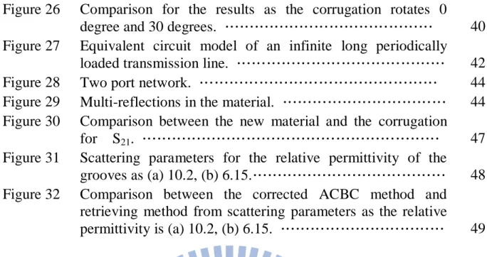
In the final section of this thesis, we will introduce the relationship between the scattering parameters and the wavenumbers. The original goal was to obtain the dispersion diagram, but when it comes to the measurement stage, unfortunately, it is impossible to measure the wavenumbers directly. So most of the time in the literature, the way to explain the width and position in the frequency spectrum of bandgaps is through the scattering parameters, which are reflection and transmission coefficient (︱S11︱ and︱S21︱). For structures that can be

represented by equivalent circuits, it is possible to get the relationship between the scattering parameters and wavenumbers by the ABCD matrix. But for more complex structures, the computation may be too elaborate. In [14], a method was described to retrieve the complex permittivity and permeability. We shall herein employ it to the scattering parameters of the corrugated surface to construct the dispersion diagram, which is then verified with the one generated by the characteristic equation derived from ACBC.

(a) (b)

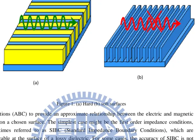
Figure 2: (a) Mushroom-like EBG structures, (b) multi-via cascaded mushroom-like EBG structures.

4

II. Theory

2-1 Characteristic equation of the corrugation

The total E and H field are obtained by the superposition of the individual field due to A and F, where A and F represent the magnetic and electric vector potential, respectively.

1 1 [ ( )] ( ) A F E E E j A



j A F





         (1) 1 1 ( ) [ ( )] A F H H H A j F



j F





         (2)

(1) and (2) can be expanded and be written as

2 2 2 2 2 2 2 2 2 2 2 2 1 1 [ ( ) ( )] 1 1 [ ( ) ( )] 1 1 [ ( ) ( )] y y x z z x x y x z x z y y y y x z x z z A F A A F E a j A j x x y x z y z A A A F F a j A j x y y y z z x A F A A F a j A j x z y z z x y



















                                                         (3a) 2 2 2 2 2 2 2 2 2 2 2 2 1 1 [ ( ) ( )] 1 1 [ ( ) ( )] 1 1 [ ( ) ( )] y y x z z x x y x z x z y y y y x z x z z F A F F A H a j F j x x y x z y z F F F A A a j F j x y y y z z x F A F F A a j F j x z y z z x y



















                                                         (3b)

Since we want the field expressions that are independent of the coordinate system, for the transverse magnetic (TM) modes, it is acceptable to let the vector potential A have only a component, and the remaining components of A as well as all of F are set to be zero. To express the surface waves on the corrugation in Fig. 3, we derive the field expressions that are TM to y. Let ( , , ) y y Aa A x y z (4a) 0 F  (4b)

5 Then 2 1 y x A E j x y       , 1 y x A H z      2 2 2 1 ( ) y y E j A y        , Hy0 2 1 y z A E j y z       , 1 y z A H x     (5)

Similarly, we let the F vector potential have only a component in the y direction, and set the remaining components F and A as zero, then we can get the transverse electric (TEy) modes. Let A0 (6a) ( , , ) z z Fa F x y z (6b) Then x 1 y F E z     , 2 1 y x F H j x y       E_y 0, 2 2 2 1 ( ) y y H j F y        E_z 1 Fy x      , 2 1 y z F H j y z       (7)

The next step is to discuss the fields for two cases, in the groove region and above the corrugations, respectively, and two different modes for each case. At first, we consider the fields within the grooves of TEy and TMy modes, and the boundary conditions are as follows:

Figure 3: Infinite-long planar corrugated surface.

p

a

o

6 ( ) 0 2 x g E z   ,E y_x( 0)0 ( ) 0 2 y g E z   ,E y_z( 0)0 (8) Also we assume the expression of the vector potential A is as:

cos sin cos sin

( , , ) [ cos( ) sin( )]{ cos[ ( )] sin[ ( )]}

2 2 xo jk x y y y y y z z z z g g F x y z e C k y C k y C k z C k z (9)

Then with (9) substituted into (5) and (7),

TE y TE _xo y TM TM groove TE groove z y x jk x groove groove groove x TM z y groove A S S E _p e g H A C C           _{ }     _{ }           (10a) 0 y TE y TM groove y groove y E H          (10b) TE y TE xo o y TM TM groove TE groove z y z _{jk x groove} x groove groove z TM z y groove A C S E jk e H A S C          _{ }  _{   }           (10c) xo y TE o TE TE y TM TM TM

groove jk x groove groove

x _{x TE y z y}

groove groove groove

groove groove x TM y z y H _{k e A k C C} u E   A k S S    _{ }        _{ }   (10d) 2 2 2 2 [ ( ) ] [ ( ) ] xo y TE TE TE y TE TM TM

groove _{jk x groove groove}

y _{TE groove y z y}

groove groove groove

groove groove y TM groove y z y H _{e A k k C S} j u E   A k k S C    _{  }        _  _   (10e) xo y TE TE TE y TE TM TM jk x

groove _{groove groove}

z _{TE y z y}

groove groove groove

groove groove z TM y z y p e H _{g A k S C} j u E A k C S       _{ }         _{ }   (10f) where cos[ ( )] 2 sin[ ( )] 2 z z p g z C g S p g z g    _              _     , and cos( ) sin( ) T T T T groove y y groove y y C k y S k y                     

7

in which ξ may be the E or H, and p is the 0,1,2….

Next we discuss the fields in the region above corrugations (y > d), and assume its vector potential A is as follows: ( ) ( , , ) e above above y z xo jkTM y d jkTM z jk x above above y TM A x yd z A  e  e (11) Then using (5) and (7) to substitute for (11)

( ) e above above y z xo TE TE y _TE TE o y TE above _{jk x jk y d jk z above} above x _z TE above above x z E _{A j e e k} k E        _{ }        _{ }   (12a) 0 y TE y TM above y above y E H          (12b) ( ) 2 2 e ( ) above above y _{o TE} TE _xo y_TE z_TE y TE TE TE TE y TE above _above x _{jk y d jk z x y} jk x above above TE above y above y

above above _{above above}

above y z z H _{k k} A e e H k k j k k H         _{  }   _{ }  _{    }   _{ }    _{ }   (12c) ( ) 2 2 e ( ) above above y _{o TM} TM _xo y_TM z_TM y TM TM TM TM y TM above _above x _{jk y d jk z x y} jk x above above TM above y above y

above above _{above above}

above y z z E _{k k} A e e E k k j k k E         _{  }   _{ }  _{    }   _{ }    _{ }   (12d) ( ) e above above y z xo TM TM y _TM TM o y TM above _{jk x jk y d jk z above} above x _z TE above above x z H _{A j e e k} k H        _{ }         _{ }   (12e)

The unit vectors parallel and orthogonal to the corrugations are defined as a_p and a , _o

respectively. According to [12], the asymptotic corrugation boundary conditions are stated as follows: ˆ 0 groove p E a  (13a) ˆ 0 above p E a  (13b) ? above groove o o E a E a (13c) ? above groove p p H a H a (13d) Assuming pTE=0 and pTM=0, i.e. we only consider the dominant mode of TE and absence

8

of all the TM modes. When pTE=0, 0

y TE groove x E  in (10a), meanwhile 0 y TM groove x E  when we

ignore the TM modes, so the boundary conditions of (13a) is automatically satisfied. As for (13b), we require ( ) ( ) 0 y y TE TM above above x x E yd E yd  (14) For phase continuity, we can get univ ₀

x x k k and

TM TE

univ above above

z z z k k k . So we can obtain univ univ x z univ jk x jk z above z TE abv jk A e e     univ univ TM x z univ above x y jk x jk z above TM abv abv k k A e e j     0 (15a) Then TM univ

above above z above

TM univ above TE x y k A A k k   (15b) As for (13c), we require 0 = 0 ( ) ( ) ( ) ( ) y y y y TE TM TE TM TE TM

groove groove above above

z z z z

p p

E y d E y d E y d E y d



       (16) in which the second term on left hand side is vanished since we assumed that no TM modes exist within the groove. Using (10c), (12a), and (12d) to substitute in (16)





0 0 0 sin univ univ x z z TE

univ univ univ univ

TM x z x z z jk x jk id groove x groove TE y i groove above univ y z jk x jk z jk x jk z above x above TE TM d

abv abv abv

jk A e k d e k k jk A e e A e e j





 

       



(17)

wherei is the groove index,noting how the left-hand side quantity varies with z in a stepwise manner, with each term of its summation being a piecewise constant within the ith groove, i.e.

idz – g/2 < z < idz + g/2. Now we only focus on the ith groove, so the summation over the groove index on the left-hand side is removed, resulting in





0 0

0

2 2

sin zuniv z TM univz

TE

z z z

above univ

y z

jk id jk z

groove x groove above x above

TE y _d TE TM g g

id z id

groove abv abv abv

k k jk jk A k d e A A e j                     (18)

And as the period dz tends to zero, the

univ z jk z

e factor on the right-hand side of (18) becomes approximately _ejkunivz idz . This expresses that the continuous variation with z can be

approximated as a piecewise discrete constant over the ith groove of nearly zero width. Hence the resultant _ejkunivz idz gets canceled out on both sides, leading to

9





0 0 sin TM TE above univ y z

groove x groove above x above

TE y TE TM

groove abv abv abv

k k

jk jk

A k d A A

j

      (19a)

Using (15b) to substitute for A_TMabove in (19a), yielding





2 2 2 ( ) sin o o TE univ x x z

groove groove above

TE y TE groove above k k k A k d A     (19b) As for (13d), we require 0 = 0 ( ) ( ) ( ) ( ) y y y y TE TM TE TM TE TM

groove groove above above

x x x x

p p

H y d H y d H y d H y d



       (20) in which again the second term on the left hand side is vanished.

To replace (20) in (10a), (10d, and (12e)





0 0 0 cos univ univ TE x z z TE

univ univ univ univ

TE x z x z z groove x y jk x jk id groove groove TE y i groove groove above univ x y jk x jk z jk x jk z above above z TE TM d

abv abv abv

k k A e k d e k k _jk A e e A e e j               



(21)

And as the same process from (17) to (19), we can modify (21), leading to





0 0

cos

TE TE

TE

groove above _univ

x y x y

groove groove above above z

TE y TE TM

groove groove abv abv abv

k k k k jk

A k d A A

j

    

    (22a)

Using (15b) to substitute for A_TMabove in (22a), yielding





2 2 2 0 ( ) cos o TE TM TE TE o TM

above above univ

groove _above

x y y above above z

x y

groove groove TE

TE y above

groove groove above above x y

k k k k k k _jA A k d k k           (22b)

As observed, we can see that since the left hand side is pure real (

TE

groove y

k is real), the right

hand side must be real. In order for this, the

TE above y k and TM above y

k must be pure imaginary such

that their product in numerator becomes real, whereas the remaining

TM

above y

k in denominator

causes the whole right hand side equation to be imaginary. This conforms with what we expect of TE above y k and TM above y

k , being wavenumbers along vertical direction perpendicularly away

from corrugation xz-surface, which should be indeed be imaginary in order for surface wave along xz plane surface of corrugation, i.e. decaying fields as one observe perpendicularly away from corrugation surface. Hence

10 TE TE above above y y

k

 

j



and TM TM above above y y

k

 

j



(23) Thus, with two replacement made, (22b) becomes





2 2 2 0 ( ) cos o TE TM TE TE o TM

univ above above

groove

above z x y y

x y

groove groove above

TE y TE above

groove groove above above x y

k k k k k A k d A k          (24) Dividing (19b) by (24)

 

 

2 2 2 2 2 tan( ) o TM o o TE TE _{o TE TM} above univ above x y x z groove x groove y

groove _{univ above above}

y _{above z x y y} k k k k k d k _{k k k}       _        (25)

The general formula for

TE groove y k is given by

  

2



2 2 TE

groove univ groove

y groove groove x z

k      k  k (26a)

Again we only consider the dominant mode under ACBC, which means pTE=pTM=0, so kzgroove

is zero, i.e. 0 groove z TE TM k  p  g p  g  , under ACBC (26b) So (26a) becomes

 

2 2 TE groove univ y groove groove x k      k , under ACBC (26c) We may equate both TE and TM attenuation constants along the vertical y direction for the upper half-space region above corrugation as the explanation just after (14), yielding

TE TM

above above above

y y _say y

   (26d)

With



_above

    

2 _univ 2 _univ 2 ₂

y kx kz abv abv

      (26e) At last, based on (26a) to (26e), we can modify (25) as

 

 

 

 

2 2 2 2 2 2 2 2 2 2 2 2 2 2 tan( ) 0 o o o o o univ univ above x z x z above groove groove x univ univ groove x above z x z above k k k k k k k d k k k k k k k  _  _   _   _{  }   _ _   _   (27) where 2

groove groove groove

k   f   ,k_above 2 f  _{abv abv} (28)

11

2-2 Refinement factor of the characteristic equation

The surface impedance looking down at y=d towards the PEC floor of the corrugations is defined as follows: ( ) ( ) y TE y TE groove TE _z groove s groove x E y d Z H y d      (29a)

substituting (10a) and (10f) into (29a), yielding





tan TE TE TE groove groove groove y s groove y Z j k d k    (29b) where TE groove groove ky

 is the familiar TEy modal impedance Zc

TE

, therefore obtaining the familiar input impedance of a shorted transmission line of length d.

Similarly, the input impedance looking up at y=d interface into the upper-half space is:

   

2 2 ₂ ( ) ( ) ( ) ( ) y y TE TE y y TE TE above above TE x z

above abv abv

s above above above

univ univ z x y x z above E y d E y d _{j j} Z H y d H y d _{k k k}              _{ } (30)

being the familiar TE modal impedance, where as

   

2 2 ₂ ( ) ( ) ( ) ( ) y y TM TM y y TM TM

above above univ univ _above

TM _{x z} x z above _y above s above above z x abv abv E y d E y d k k k Z H y d H y d j j                (31)

being the familiar TM modal impedance.

The whole Ex and Ez in the numerators of the expressions for these impedances seems exist,

but actually it is only under the ACBC conditions. As mentioned, ACBC is an approximate method to analyze corrugation, and its hypothesis is that we assume the ridge is tending to zero. For the real case, there exist widths for the ridges, so (27) may produce some errors in its results compared to the simulation or measurement The Ex and Ez vanish over the top PEC

surfaces of the metallic ridge, hence, it is fairly presumed that the Eabove fields on the corrugation surface may be corrected by an incremental (> 1) factor dz/g, where dz is the corrugation period and g is the groove-width. By doing this, in reality, the Eabove fields on the corrugation surface with the reduction factor (< 1) (as required by the fractional existence of the tangential E-field components over only apertures of the grooves, and vanishing over the ridge-top) will neutralize that aforementioned incremental factor, thereby maintaining the abovementioned impedances, since there is no for these impedances to be changed.

The equation containing Eabove should all be modified, which are (14) and (16), and it can be seen that this multiplicative correction factor would get canceled throughout (14), meaning that only (16) should be modified, which is

12

( ) ( ) ( )

y y y

TE TE TM

groove z above above

z z z d E y d E y d E y d g     _    _ (32a) again using (10c), (12a), and (12d) to substitute in (32a), obtaining





0 0 sin TM 0 TE above univ y z

groove x groove above z x above z

TE y TE TM

groove abv abv abv

k k

jk d jk d

A k d A A

g g j

       (32b)

so the last characteristic equation is also changed to

 

 

 

 

2 2 2 2 2 2 2 2 2 2 2 2 2 2 tan( ) 0 o o o o o univ univ above x z x z above groove z groove x univ univ groove x above z x z above k k k k k d k k d g _{k k k k k k k}  _  _   _   _{  }   _ _   _   (33)

Depending on which two of the following three quantities: (i) frequency f = ω/(2π), (ii)

univ x

k , and (iii) univ z

k we choose, the third quantity remains as the only unknown in this (33), which may then be solved for as roots of this characteristic equation. Doing so yields the required information for plotting various path-regions of the dispersion diagram (OZ,

ZM, MX, or XO). If we know the frequency and set univ

x

k as zero, we can get the root of univ

z

k , which is the OZ of the dispersion diagram, where Z refers to the Brillouin limit, π / dz. Similarly, setting the kuniv_z as Brillouin limits, and solve the root for, we can get ZM part.

The dispersion diagrams generated by the present ACBC-based method are compared with commercial full-wave simulator software: CST Microwave Studio® . Two arbitrary examples shall be studied as follow.

2-3-1 An arbitrary example

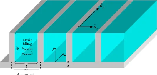
The parameters are as follow: period dz = 2mm, groove-width g = 0.85*dz, depth d = 8mm,

εrel,groove = 2 and μrel,groove = 1. As seen, the roots of the characteristic equation produce a dispersion trace which takes on the form of cyclic „peaking‟ of the kzuniv at various resonant frequencies in Fig. 4(a). Moreover, the trace just „grazes‟ the light-line, i.e. it is tangent to it, occurring at frequencies slightly above those whereby the trace has dropped back to its local minima and begun to rise again. In fact, the backward trace of the dispersion diagram in Fig. 4(a) is not exist, the reason why it appears is because the magnitude of the „backward‟ part is small, and even though it is small, the algorithm we used in Matlab still can detect these roots. The comparison to the CST simulation results will be shown in the next section, and we will see that no backward trace is shown in the simulation results.

Interesting aspect is now pointed out. The frequencies at which the peaks occur coincide perfectly with the so-called “soft” frequencies [3] of the corrugations, defined as

13

Figure 4 (a):OZ path of the dispersion diagram

14



2 1





4 ,



soft

n soft rel groove

f c n d 

(34) where n is an integer representing the order of the soft boundary condition, c is the speed of light in vacuum, dsoft is the depth of the corrugations at which the soft boundary condition holds, and εrel,groove is the relative permittivity of the dielectric filling the grooves.

2-3-2 ACBC method compared to CST

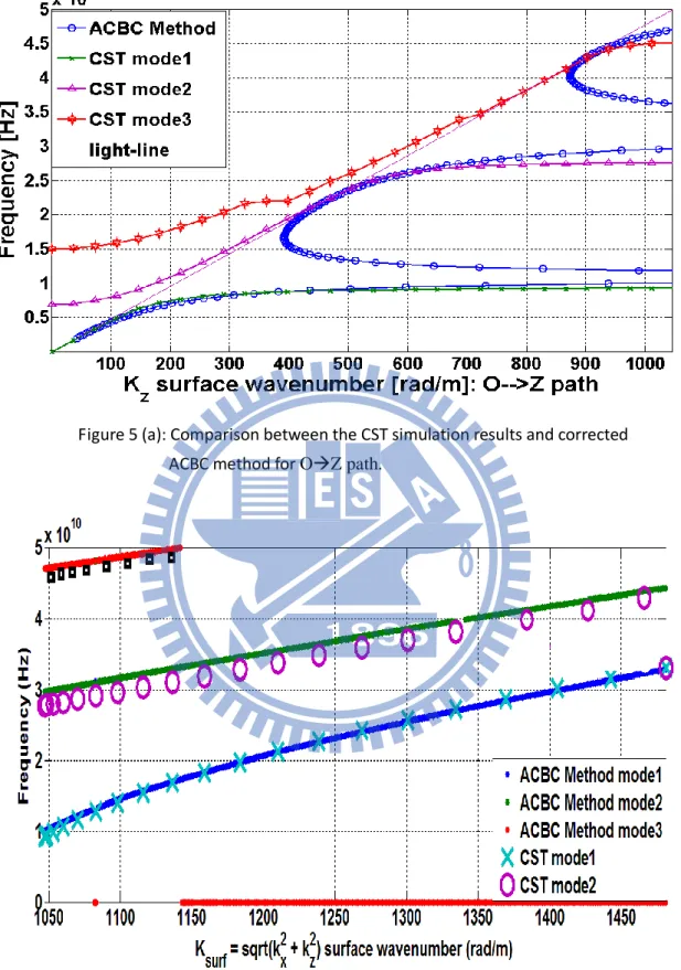
The parameters are as follow: period of the unit cell dz = 3mm, groove-width g = 0.55*dz, depth d = 4mm, εrel,groove = 3 and μrel,groove = 1. The dispersion diagram obtained in this section is from Eq. (38), which are corrected characteristic equation, but not Eq. (27), and we will see the good match between the corrected ACBC methods and CST. The comparison between the uncorrected and corrected ACBC methods will be discussed in the next section. As additional results and still on this second example, the dispersion graphs for three other paths of the typical “OXMYO” dispersion diagram typical of two-dimensional periodic EBG structures are given in Figs. 5(b), 5(c), and 5(d), providing the “XM”, “MY”, and “YO” (ZM, MX, and XO for the present example) portions, respectively. However, for the present case of corrugations, there is actually no periodicity in the direction (x here) along them. Nonetheless, we shall still set the Brillouin limit along this direction as π divided by the same period (along z) of the corrugations, thus assuming a square unit cell (although strictly, the unit cell is an infinitely long strip in the zx plane of the corrugations, infinitely long along x, the orientation of the corrugations). For the “OX” (OZ for the present example) part shown in Fig. 5(a), as observed, only the rising parts of the „peaking‟ trace after the „grazing‟ are relevant, which is because just as mentioned, the algorithm we use may detect some small deviated data which are negligible. But the comparisons between the present ACBC method and CST for all three graphs of Fig. 5(b) through 5(d) demonstrate fine agreement, thereby further substantiating the present technique.

15

Figure 5 (a): Comparison between the CST simulation results and corrected ACBC method for OZ path.

Figure 5 (b): Comparison between the CST simulation results and corrected ACBC method for ZM path.

16

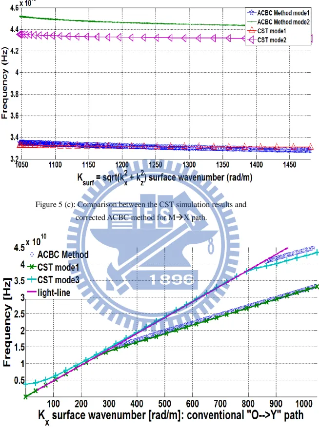
Figure 5 (c): Comparison between the CST simulation results and corrected ACBC method for MX path.

Figure 5 (d): Comparison between the CST simulation results and corrected ACBC method for OX path (conventional OY path.).

17

2-4 Influence of refinement factor

In this section, the accuracy of the refinement factor for the characteristics equation will be shown, and we study the OZ part first. The parameters we choose are as follows: dz = 1mm,

d = 5mm, εrel,groove = 3, μrel,groove = 1, and comparing two different example which are g/dz =0.2 and g/dz =0.7. Just as mentioned, ACBC is an “approximate” method to analyze the corrugation, and the approximation is that ridge tends to be zero. In other words, if the width of the ridge is larger in a period, the result showed by uncorrected ACBC methods will be more inaccurate, so that is why we need the refinement factor. Fig. 6(a) and Fig. 6(b) show the comparison of the dispersion diagram for the OZ part resulting from Eq. (27) (uncorrected ACBC methods) and Eq. (33) (corrected ACBC methods), and both are discussed in two cases which are g/dz =0.2mm and g/dz =0.7mm, respectively. Since the accuracy of the corrected ACBC methods has been proven in the last section, it will be used as a standard here. It can be seen that no matter what value of g/dz is, it does not affect the dispersion diagram resulting from ACBC method without correction method, and for which is not so practical. As the groove width gets smaller, which means the condition gets farther than the uncorrected ACBC, the improvement effects from the correction factor gets better. The similar situations also happened to the ZM part, which are shown in Fig 7(a) and Fig 7(b). In fact, from our simulation results for the entire parametric space, we found that the accuracy

Figure 6(a): Comparison between the uncorrected and corrected ACBC method for OZ path as the g/dz =0.2.

18

Figure 6(b): Comparison between the uncorrected and corrected ACBC method for OZ path as the g/dz =0.7.

Figure 7(a): Comparison between the uncorrected and corrected ACBC methods for ZM path as the g/dz =0.2.

19

of the unrefined ACBC method is properly satisfactory when g/dz is greater than 0.7, but degrades rapidly as the ratio falls below this threshold value, for which the refined dispersion relation of Eq. (33) would then be required.

2-5 ACBC method compared to TRT

Actually, the dispersion diagram of the corrugation has been investigated decades ago, which is transverse resonant technique (TRT). The characteristic equation is obtained by matching impedance in [15], whereas with the assumption that only the TM modal exist for y>d. We will briefly introduce how its characteristic equation comes.

The impedance looking upward is that of a TM wave propagating in the y-direction, yielding y upward o k Z   (35) the impedance looking down into the corrugation would be





tan r downward groove r jW Z k d W t     (36)

where W is the period and t is the ridge width, We can see that (36) is quite similar to (29b),

Figure 7(b): Comparison between the uncorrected and corrected ACBC methods for ZM path as the g/dz =0.7.

20

the former one is for TM modal while the latter one is for TE modal, and also (36) has already considered the incremental factor W

Wt .

So by TRT theory, matching impedance at y=d requires that

upward downward Z  Z (37) resulting in

 

2 2 ₂





0 0 0 0 4 4 rg tan 2 z g g rg W f k f fd W t                _{ }    (38)

for OZ part. And

 

_{ }

 

2 2 2 0 0 2 0 0 2 2 2 0 0 4 tan 4 4 x rg rg rg x rg z x W f k d f k W t k k f               _{  }   _{ }       (39) for ZM part.

Figs. 8 show the comparison between the ACBC method and TRT method which is from the book written by Carlton H Walter. The dimension is the same as Fig. 5(a). We can see from Fig. 8(a), for OZ part, TRT method matches well to the corrected ACBC methods, and also the information is obtained that corrected ACBC method really improves the accuracy for the uncorrected ACBC method (since we have already proved in Fig. 5(a) that corrected ACBC method matches well to the CST software, we use the former one as the standard). Just like the ACBC method, the cyclical „peaking‟ of the kz at various resonant frequencies is also exhibited by the TRT, and its traces also just „graze‟ the light-line, i.e. are tangent to it. However, Fig. 8(b) for oblique surface-wave propagation reveals that the TRT leads to severe errors in the dispersion diagrams. Only at the Bragg condition (Brillouin limit), i.e. left edge of Fig. 8(b) that links to the right edge of Fig. 8(a), will the accuracy of the TRT be satisfactory, but degrades rapidly as the surface wave vector departs from the principal direction. For such acute inaccuracies, even the uncorrected ACBC method of (27) provides better characterization of oblique surface wave propagation.

21

Figure 8(a): Comparison between the corrected ACBC method and TRT for OZ path.

Figure 8(b): Comparison between the corrected ACBC method and TRT for ZM path.

22

2-6 Field distributions

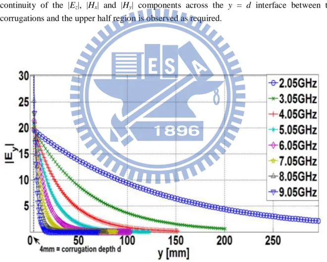
Fig. 9(a) and 9(b) show the variation of the magnitude of the E-field components against the vertical y-direction for various frequencies within the first surface wave passband (0 to 10GHz according to Fig. 5(a)), whereas the graphs of Figs. 10. are for the H-field components. As the frequency rises and moves deeper into the first surface-wave regime (2.05 through 9.05 GHz in 1GHz steps, as selected for plotting), the corresponding increased surface-wave phase constant univ

z

k beyond k_above  _{abv abv} and thus strengthened attenuation constant

above y

 along the vertical y direction is indeed demonstrated by the progressively steepened exponential decay of the various field components with increasing frequency. In addition, the continuity of the |Ez|, |Hx| and |Hy| components across the y = d interface between the corrugations and the upper half region is observed as required.

23

Figure 9(b): |Ez| plotted against y-direction

24

Figure 10(b): |Hy| plotted against y-direction

25

III. Sectorial band gap

3-1 Dispersion diagram corresponding to Brillouin zone

For most of the studies in the literature, the EBG structures usually are used to deal with the entire bandgap, i.e. within the certain frequency bands, the surface waves are all suppressed on the EBG surfaces. There are potentially some applications which do not need a bandgap for all directions but just certain directions. Despite not potentially able to provide entire bandgap, planar corrugated surfaces are classically known to possess the capacity of offering surface-wave pass-bands and stop-bands along the directions parallel and perpendicular to the grooves and ridges, respectively, which are known as hard and soft surfaces as mentioned. However, no works have yet studied their candidature for serving as sectorial bandgap structures. We will demonstrate that planar corrugations are able to exude this capability. By capitalizing on the rapid surface-wave solution provided by the ACBC, we shall use the planar corrugated surface as the vehicle to illustrate how sectorial bandgap structures can be designed efficiently. This is something which no other periodic structures without analytic surface-wave solutions can readily afford.

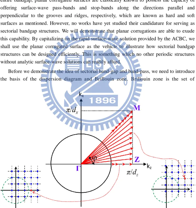
Before we demonstrate the idea of sectorial band-gap and band-pass, we need to introduce the basis of the dispersion diagram and Brillouin zone. Brillouin zone is the set of

φ

k

z

k

x

26

wavenumbers which can describe the propagation of electromagnet ic waves in two-dimension photonic crystals, as shown in Fig.11, where k0 is the wavenumber in free

space.Since we only consider the surface wave, the wavenumber which is vertical to the corrugation must be pure imaginary, which leads to

2 2

0

surface x z

k  k k k (40)

so we just need to consider the region outside the circle for the surface wave case. As shown in Fig 11, each arrow constitutes a certain surface wavenumber for a certain frequency, but for the most important aspect here, there is not just only one surface-wave vector-arrow for any one certain frequency. This will be discussed deeper later.

In Section II, we show four parts (O→Z, Z→M, M→X, and X→O) of the dispersion diagram. As mentioned, any one of these parts is obtained by fixing two of these three unknowns, (i) kx, (ii) kz and (iii) frequency, and then the roots for the remaining unknown are

solved for. If we set kx as an unknown, and set

tan( )

x z

k



k



(41)

where φ is the angle between the propagation path of the surface wave and the z axis. Then

27

the roots for kz are solved we can get the dispersion diagram for the surface waves

propagating along the path which has φ degrees with the z-axis. For the extreme case, we can take the X→O part as the 90 degrees cases turning from O→Z part. Two arbitrary different examples are shown in Fig. 12, the dimensions are as follows: dz = 3mm, d=4mm, εrel,groove = 3 and the values of φ are 10 and 45 degrees, respectively.

3-2 Concept of sectorial bandgap

Refer to the fictitious dispersion diagram in Fig. 13 below, which shows traces for various azimuth  (measured from the z-axis perpendicular to the corrugations) directions of surface-wave modal propagation, i.e. each trace pertaining to a certain fixed , with the original dispersion paths of OZ, Zbeyond included for reference. Let the frequency corresponding to the Brillouin limit be denoted as f1. The associated surface-wavevector at

this frequency is shown by the arrow in Fig. 14 with magnitude ksurf f1 = /dz and directed along z perpendicular to the corrugations. As the surface-wavevector enters the oblique nonzero  regime ( measured from the z-axis perpendicular to the corrugations), but with kz maintained at /dz, i.e. now the surface-wavevector component along z (kz) is no longer zero,

28

both the eigen-frequency and modal surface-wavenumber increases further, the relationship between them as indicated by the traces corresponding to ksurf values greater than ksurf f1 = /dz. For illustration, the surface wavevector at an example frequency of f2 (labeled in Fig. 13) is

represented in Fig. 14 by the arrow with magnitude ksurf f2. Due to symmetry about both horizontal and vertical axes, two arrows with magnitude ksurf f2 are shown in Fig. 14 (the same applies for other oblique surface-wavevectors). As the frequency rises further up to the point where the next higher-order surface-wave mode starts to emerge at f3 as shown in Fig. 13, the

surface-wavevector is directed towards an even larger  angle as represented by the arrow with magnitude ksurf f3 in Fig. 14.

As it can be seen in Fig.13, the original stopband region for zero angular span (phi=0) is between f1 and f3, and for the case when phi is “φb” degrees, the stopband zone is from f2 to f3,

so it means as the phi gets larger, the stopband areas get smaller. In other words, we can say that during the period from f2 to f3, there is “at least” “φb” degrees sectorial band gap area. It

is easily misunderstanding the above idea in another expression which is Brillouin zone as shown in Fig.14. The sectorial bandgap angle (SBGA, in degrees) is between f1 and f2, but not

between f2 and f3. Also by applying the above idea, we can define the boundary between the conventional soft and hard surfaces, which is the surface-wavevector ksurf f3 in Fig.14, i.e. the sectorial bandgap angle corresponding to the frequency which the next mode just appears.

Fr eq u en cy f1 f2 f3 O SBGW = f3 – f2 ksurf [rad/m]

k

surf f1

=



/d

Z Light line Specified Specified a b c a b c fa fb = d fc fd =

Figure 13: Fictitious dispersion diagram  = 0