心電圖訊號的渦漩和適應性多速率壓縮

國

立

交

通

大

學

電信工程學系

碩

士

論

文

心電圖訊號的渦漩和適應性多速率壓縮

Turbo and Adaptive Multirate Compressions of

Electrocardiogram Signals

研 究 生：施泓瑋

指導教授：蘇育德 博士

心電圖訊號的渦漩和適應性多速率壓縮

Turbo and Adaptive Multirate Compressions of

Electrocardiogram Signals

研 究 生：施泓瑋

Student：Hong-Wei Shih

指導教授：蘇育德 博士 Advisor：Dr. Yu T. Su

國立交通大學

電信工程學系碩士班

碩 士 論 文

A Thesis Submitted to

Department of Communication Engineering

College of Electrical and Computer Engineering

National Chiao Tung University

In Partial Fulfillment of the

Requirements for the Degree of

Master of Science

In Communication Engineering

Hsinchu, Taiwan, Republic of China

September 2006

心電圖訊號的渦漩和適應性多速率壓縮

研究生: 施泓瑋 指導教授: 蘇育德 博士 國立交通大學電信工程學系碩士班 中文摘要 本文提出兩種新型的心電圖訊號壓縮技術。第一種方式應用了迭代式 (iterative)通道解碼的渦輪原理(turbo principle)，而第二種方式則借用了最新的標 準語音編碼法，即適應性多速率寛頻編碼。後者可提供較佳的壓縮比但前者較適 合於合併式的訊源通道編碼。 無失真的壓縮是透過將渦輪編碼器輸出加以適當的穿刺(puncture)後再經迭 代式解碼還原。穿刺的比率會逐漸上升直到無法達到零失真還原為止。因為正交 轉換可提供心電圖訊號一種有用的表示法，能夠很簡單的區隔數據的重要性，我 們先用離散餘弦轉換(DCT)將心電圖數據轉換之後，再透過上述的渦輪壓縮過 程，依轉換後數據之重要性來作穿刺，穿刺後的數據復利用渦輪（迭代式）解碼 法去檢測訊源端的完整性和可回復性來確定資料源是可正確無誤的重建。為避免 壓縮後的數據因為在傳輸過程遭到雜訊干擾無法正確解碼，我們可以在傳輸端加 入部份原先穿刺掉的（通常是重要較高的部份）位元用來抵抗雜訊。這種合併訊 源通道的編碼方式只需要單一的編解器，在解碼器也不需要訊源的參數（如其先 驗機率分佈），即可從事迭代解碼。 除此之外，我們也利用所謂「適應性多速率寬頻編碼法」提出一種新穎的心 電圖壓縮方法。「適應性多速率寬頻編碼法」在語音壓縮方面己經有很顯著的成 功。我們修正了這種方法從另一種觀點來處理一維的心電圖訊源。我們是利用碼 激勵線性預測(CELP)編碼為基型(合成分析法)來作心電圖的編碼。首先，我們利 用長時距預測濾波器(Long Term Predictor)得到心電圖訊號的近似週期和增益。心 電 圖 訊 號 經 長 時 距 預 測 濾 波 器 後 的 訊 號 會 先 通 過 短 時 距 預 測 (Short Term Predictor)濾波器，再以後者的輸出建立碼簿(Codebook)。如此一來，我們只需傳 送長時距預測濾波器和短時距預測濾波器的係數以及建立出來的碼簿的索引便 可重建原始信號。電腦模擬的結果顯示這種方法對心電圖壓縮非常有效，在均方 根誤差百分比約為３％的要求下，可達到壓縮比率 30 左右。

Turbo and Adaptive Multirate Compressions of

Electrocardiogram Signals

Student : Hong-Wei Shih Advisor : Yu T. Su

Department of Communication Engineering National Chiao Tung University

Abstract

Several recent publications have shown that joint source-channel decoding could be a powerful technique. In the first part of this thesis, we propose the use of punctured turbo codes with the idea of unequal error protection (UEP) to perform lossless compression and joint source channel coding of ECG data using the discrete cosine transform (DCT), because orthogonal transforms provide alternate signal representations that can be useful for electrocardiogram (ECG) data compression. Compression is achieved by puncturing the turbo code to the desired rate. We use the turbo principle to iteratively estimate the source integration and to compensate the error due to compression. No information about the source distribution is required in the encoding processing. Moreover, the source parameters do not need to be known in the decoder, since that can be estimated jointly with the iterative decoding process. We also present an useful puncturing method, which ensures the compression of ECG data in a predetermined number of reconstruction attempts.

The second part of this thesis presents a novel approach for compression of ECG signals based on the adaptive multi-rate wideband codec method. Adaptive multi-rate wideband codec method has achieved prominent success in speech compression. Here we use a modified version of adaptive multi-rate wideband codec method for one dimensional

signals. We applied adaptive multi-rate wideband codec method on different records of ECG signal database. Numerical experiments show that this method has a very high efficient compression performance. Using the percent-root-mean-square distortion (PRD) measure, the coder is shown to give a compression ratio about 30 with a PRD less than 3.0%.

Contents

English Abstract i

Contents iii

List of Figures v

1 Introduction 1

2 Electrocardiogram Data Compression Method 3

2.1 Introduction to Electrocardiogram (ECG) . . . 5

2.2 Direct ECG Data Compression Schemes . . . 10

2.3 Transformation ECG Data Compression Schemes . . . 12

2.4 Transform Representation . . . 13

3 Joint Turbo Source and Channel Coding 16 3.1 Decremental Redundancy–Source Coding . . . 17

3.2 Source Decoding . . . 20

3.3 Designing the Puncture Table: A Dual of Unequal Error Protection . . . 21

3.4 Upper Bounds of Discrete Cosine Transform . . . 23

3.5 Joint Source and Channel Coding Using Unequal Protection . . . 25

3.5.1 Simulation Results . . . 31

4 Adaptive Multirate Approach for Electrocardiogram Compression 34 4.1 The Code Excited Linear Prediction Coder . . . 35

4.1.1 Linear Prediction Analysis . . . 35

4.1.2 Line Spectral Frequencies . . . 39

4.1.3 Codebook Generation . . . 41

4.2 Using the Idea of AMR-WB for Compression of ECG Signals . . . 45

4.2.1 Encoder . . . 45

4.2.2 Decoder . . . 48

4.2.3 Simulation Results . . . 49

5 Conclusion 53

List of Figures

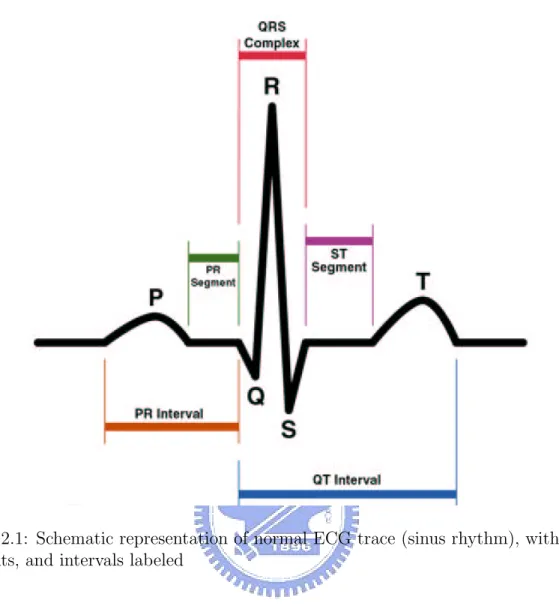
2.1 Schematic representation of normal ECG trace (sinus rhythm), with waves,

segments, and intervals labeled . . . 7

2.2 Input signal . . . 14

2.3 Signals spectrum after discrete cosine transform. . . 15

3.1 Lossless compression of a source block using turbo codes. Compression is achieved by puncturing and verifying the integrity of the reconstructed source sequence. . . 17

3.2 A parallel concatenation of rate 1 convolutional codes (CC) with an inter-leaver between them followed by heavy puncturing can be used to perform data compression of binary sources. . . 18

3.3 Puncturing scheme for decremental redundancy. . . 18

3.4 Parallel turbo source decoder. . . 20

3.5 Signals spectrum after discrete cosine transform. . . 25

3.6 Signals spectrum after discrete cosine transform. . . 26

3.7 Block diagram of turbo-principle-based ECG compression . . . 26

3.8 Block diagram of turbo-principle-based encoder . . . 31

3.9 Compression with joint turbo source and channel coding . . . 32

3.10 Average PRD comparison between proposed method and wavelet trans-form with arithmetic coding and rate-1/2 turbo coding . . . 33

4.2 Formant prediction. . . 37

4.3 Pitch prediction . . . 38

4.4 One dimensional VQ . . . 42

4.5 Two dimensional VQ . . . 42

4.6 Detailed block diagram of the encoder . . . 46

4.7 Detailed block diagram of the decoder . . . 47

4.8 ECG compression performance using the adaptive multi-rate wideband codec method . . . 50

4.9 ECG compression performance using the adaptive multi-rate wideband codec method . . . 51

4.10 ECG compression performance using the adaptive multi-rate wideband codec method . . . 52

Chapter 1

Introduction

Conventional source codes, e.g. Huffman codes or arithmetic codes, remove re-dundancy very efficiently and thus achieve compression rates very close the theoretical limit–the entropy rate of the source. However, these methods are very sensitive to errors such as those resulted from the re-synchronization process.

During the last decade, robust source coding techniques based on forward error correcting codes have been introduced. Approaches based on low-density parity-check (LDPC) codes were studied in [1], [2], whereas [3], [4] concentrated on source coding using turbo codes. Their common success relies on the usage of a probability-based message-passing algorithm during decoding.

It is well known that data compression and data transmission are essentially dual problems. In compression (source coding) we remove all the redundancy in the data to form the most compressed version possible whereas in transmission (channel coding) over noisy channels we add redundancy in a controlled fashion to combat errors in the channel.

Turbo codes form a class of very powerful channel codes that yield near-Shannon limit performance. The principle of turbo (iterative) decoding has been applied to areas other than channel codes. More recently, the turbo principle has been applied successfully to data compression of binary memoryless sources. Source coding schemes based on the turbo principle can be easily extended to obtain powerful joint source-channel codes for

point-to-point transmission [5]. In the first part of this thesis we present a joint turbo source and channel coding scheme for ECG signals. The spectral property of ECG signals is used for designing puncture patterns for turbo compression and a compression ratio of 10 is achieved.

An apparent similarity between speech and ECG signals suggests that it is feasible to apply speech coding technologies to ECG data compression. The so-called Adaptive Multi-Rate Wideband (AMR-WB) method has been proved to be very efficient for speech coding and has been adopted as an industrial standard. The main idea is to compact the signal energy in much less samples than in the original wave samples. In the second part of this thesis, we report our findings about a modified AMR-WB approach for ECG data compression.

The outline of this thesis is as follows. In the ensuing section, we describe the strategy we adopted in presenting the existing ECG data compression schemes and introduce some properties about the ECG wave. The concepts of decremental redundancy and the associated decoding method are presented and our coding scheme is introduced in Section 3,. In Section 4, we provide detailed description of the Adaptive Multi-Rate Wideband codec algorithm and apply it for ECG signal compression.

Chapter 2

Electrocardiogram Data

Compression Method

The main goal of any compression technique is to achieve maximum data volume reduction while preserving the significant signal morphology features upon reconstruc-tion. A broad spectrum of techniques for electrocardiogram (ECG) data compression have been proposed during the last four decades. Such techniques have been vital in reducing the digital ECG data volume for storage and transmission. These techniques are essential to a wide variety of applications ranging from diagnostic to ambulatory ECG’s. Due to the diverse procedures that have been employed, comparison of ECG compression methods is a major problem. Present evaluation methods preclude any direct comparison among existing ECG compression techniques. ECG data compression schemes are presented in two major groups: direct data compression and transforma-tion methods. The direct data compression techniques are: ECG differential pulse code modulation and entropy coding, AZTEC, Turning-point, CORTES, Fan and SAPA al-gorithms, peak-picking, and cycle-to-cycle compression methods. The transformation methods briefly presented, include: Fourier, Walsh, and K-L transforms. The theoreti-cal basis behind the direct ECG data compression schemes are presented and classified into three categories: tolerance-comparison compression, differential pulse code modu-lation (DPCM), and entropy coding methods.

different conditions and constraints. Independent databases, with ECG’s sampled and digitized at different sampling frequencies ( 100 − 1000 Hz) and precisions (8 − 12 bits), have been mainly employed. The reported compression ratios (CR) have been strictly based on comparing the number of samples in the original data with the resulting com-pression parameters without taking into account factors such as bandwidth, sampling frequency, precision of the original data, wordlength of compression parameters, recon-struction error threshold, database size, lead selection, and noise level.

Each compression scheme is presented in accordance to the following five issues: a) a brief description of the structure and the methodology behind each ECG compression scheme is presented along with any reported unique advantages and disadvantages. b) The issue of processing time requirement for each scheme has been excluded. In light of the current technology, all ECG compression techniques can be implemented in real-time environments due to the relatively slow varying nature of ECG signals. c) The sampling rate and precision of the ECG signals originally employed in evaluating each compression scheme are presented along with the reported compression ratio. d) Since most of the databases utilized in evaluating ECG compression schemes are nonstandard, database comparison has been excluded. We believe such information does not provide additional clarity and at times may be misleading. However, every effort has been made to include comments on how well each compression scheme has performed. The intent is to give the reader a feeling for the relative value of each compression technique. e) Finally, the fidelity measure of the reconstructed signal compared to the original ECG has been primarily based on visual inspection. Besides the visual comparison, many compression schemes have employed the percent root-mean-square difference (PRD). The PRD value for each compression scheme is presented whenever it is available. The PRD calculation

is as follows: P RD = v u u u u u u u t n X i=1

[xorg(i) − xrec(i)]2 n

X

i=1

x2_org(i)

∗ 100 (2.1)

where xorg and xrec are samples of the original and reconstructed data sequences.

2.1

Introduction to Electrocardiogram (ECG)

An electrocardiogram (ECG or EKG, abbreviated from the German Elektrokardio-gramm) is a graphic representation produced by an electrocardiograph, which records the electrical voltage in the heart in the form of a continuous strip graph. It is the prime tool in cardiac electrophysiology, and has a prime function in screening and diagnosis of cardiovascular diseases. An ECG is constructed by measuring electrical potential be-tween various points of the body using a galvanometer. Leads I, II and III are measured over the limbs: I is from the right to the left arm, II is from the right arm to the left leg and III is from the left arm to the left leg. From this, the imaginary point V is constructed, which is located centrally in the chest above the heart. The other nine leads are derived from potential between this point and the three limb leads (aVR, aVL and aVF) and the six precordial leads (V₁₋₆).

Therefore, there are twelve leads in total. Each, by their nature, record information from particular parts of the heart:

• The inferior leads (leads II, III and aVF) look at electrical activity from the vantage point of the inferior region (wall) of the heart. This is the apex of the left ventricle. • The lateral leads (I, aVL, V5 and V6) look at the electrical activity from the vantage

point of the lateral wall of the heart, which is the lateral wall of the left ventricle. • The anterior leads, V1 through V6, and represent the anterior wall of the heart, or

• aVR is rarely used for diagnostic information, but indicates if the ECG leads were placed correctly on the patient.

Understanding the usual and abnormal directions, or vectors, of depolarization and repolarization yields important diagnostic information. The right ventricle has very little muscle mass. It leaves only a small imprint on the ECG, making it more difficult to diagnose than changes in the left ventricle.

The leads measure the average electrical activity generated by the summation of the action potentials of the heart at a particular moment in time. For instance, during normal atrial systole, the summation of the electrical activity produces an electrical vector that is directed from the SA node towards the AV node, and spreads from the right atrium to the left atrium (since the SA node resides in the right atrium). This turns into the P wave on the EKG, which is upright in II, III, and aVF (since the general electrical activity is going towards those leads), and inverted in aVR (since it is going away from that lead).

A typical ECG tracing of a normal heartbeat consists of a P wave, a QRS complex and a T wave, is shown in Fig. 2.1. A small U wave is not normally visible.

1. Axis

The axis is the general direction of the electrical impulse through the heart. It is usually directed to the bottom left (normal axis: −30o _{to +90}o_{), although it can}

deviate to the right in very tall people and to the left in obesity.

• Extreme deviation is abnormal and indicates a bundle branch block, ventric-ular hypertrophy or (if to the right) pulmonary embolism.

• It also can diagnose dextrocardia or a reversal of the direction in which the heart faces, but this condition is very rare and often has already been diag-nosed by something else (such as a chest X-ray).

Figure 2.1: Schematic representation of normal ECG trace (sinus rhythm), with waves, segments, and intervals labeled

2. P wave

The P wave is the electrical signature of the current that causes atrial contraction. Both the left and right atria contract simultaneously. Its relationship to QRS complexes determines the presence of a heart block.

• Irregular or absent P waves may indicate arrhythmia. • The shape of the P waves may indicate atrial problems. 3. QRS

The QRS complex corresponds to the current that causes contraction of the left and right ventricles, which is much more forceful than that of the atria and involves

more muscle mass, thus resulting in a greater ECG deflection. The duration of the QRS complex is normally less than or equal to 0.10 second. The Q wave, when present, represents the small horizontal (left to right) current as the action potential travels through the interventricular septum.

• Very wide and deep Q waves do not have a septal origin, but indicate my-ocardial infarction that involves the full depth of the myocardium and has left a scar.

The R and S waves indicate contraction of the myocardium itself.

• Abnormalities in the QRS complex may indicate bundle branch block (when wide), ventricular origin of tachycardia, ventricular hypertrophy or other ven-tricular abnormalities.

• The complexes are often small in pericarditis or pericardial effusion. 4. T wave

The T wave represents the repolarization of the ventricles. The QRS complex usually obscures the atrial repolarization wave so that it is not usually seen. Elec-trically, the cardiac muscle cells are like loaded springs. A small impulse sets them off, they depolarize and contract. Setting the spring up again is repolarization (more at action potential). In most leads, the T wave is positive.

• Inverted (also described as negative) T waves can be a sign of disease, al-though an inverted T wave is normal in V1 (and V2-V3 in African-Americans/Afro-Caribbeans).

• T wave abnormalities may indicate electrolyte disturbance, such as hyper-kalemia or hypohyper-kalemia.

• This segment ordinarily lasts about 0.08 second and is usually level with the PR segment. Upward or downward displacement may indicate damage to the cardiac muscle or strain on the ventricles. It can be depressed in ischemia and elevated in myocardial infarction, and upslopes in digoxin use.

5. U Wave

The U wave is not always seen. It is quite small, and follows the T wave by definition. It is thought to represent repolarization of the papillary muscles or Purkinje fibers. Prominent U waves are most often seen in hypokalemia, but may be present in hypercalcemia, thyrotoxicosis, or exposure to digitalis, epinephrine, and Class 1A and 3 anti-arrhythmics, as well as in congenital long QT syndrome and in the setting of intracranial hemorrhage. An inverted U wave may represent myocardial ischemia or left ventricular volume overload.

6. QT interval

The QT interval is measured from the beginning of the QRS complex to the end of the T wave. A normal QT interval is usually about 0.40 seconds. The QT interval as well as the corrected QT interval are important in the diagnosis of long QT syndrome and short QT syndrome. The QT interval varies based on the heart rate, and various correction factors have been developed to correct the QT interval for the heart rate. The most commonly used method for correcting the QT interval for rate is the one formulated by Bazett and published in 1920. Bazett’s formula is QTc = √QT_RR , where QTc is the QT interval corrected for rate, and RR

is the interval from the onset of one QRS complex to the onset of the next QRS complex, measured in seconds. However, this formula tends to not be accurate, and over-corrects at high heart rates and under-corrects at low heart rates. 7. PR interval

of the QRS complex. It is usually 0.12 to 0.20 seconds. A prolonged PR indicates a first degree heart block, while a shorting may indicate an accessory bundle that depolarizes the ventricle early, such as seen in Wolff-Parkinson-White syndrome.

2.2

Direct ECG Data Compression Schemes

This section presents the direct data compression schemes developed specifically for ECG data compression, namely, the AZTEC, Fan/SAPA, TP, and CORTES ECG compression schemes.

1. The AZTEC Technique: The amplitude zone - time epoch coding (AZTEC) al-gorithm originally developed by Cox et al. [6] for preprocessing real-time ECGs for rhythm analysis. It has become a popular data reduction algorithm for ECG monitors and databases with an achieved compression ratio of 10: 1 (500 Hz sam-pled ECG with 12 b resolution). However, the reconstructed signal demonstrates significant discontinuities and distortion. In particular, most of the signals distor-tion occurs in the reconstrucdistor-tion of the P and T waves due to their slow varying slopes. The AZTEC algorithm converts raw ECG sample points into plateaus and slopes. The AZTEC plateaus (horizontal lines) are produced by utilizing the zero-order interpolation (ZOI). The stored values for each plateau are the amplitude value of the line and its length (the number of samples with which the line can be interpolated within aperture ² ). The production of an AZTEC slope starts when the number of samples needed to form a plateau is less than three. The slope is saved whenever a plateau of three samples or more can be formed. The stored values for the slope are the duration (number of samples of the slope) and the final elevation (amplitude of last sample point). Signal reconstruction is achieved by expanding the AZTEC plateaus and slopes into a discrete sequence of data points. Even though the AZTEC provides a high data reduction ratio, the fidelity of the reconstructed signal is not acceptable to the cardiologist because of the

discon-tinuity (step-like quantization) that occurs in the reconstructed ECG waveform. A significant reduction of such discontinuities is usually achieved by utilizing a smoothing parabolic filter. The disadvantage of utilizing the smoothing process is the introduction of amplitude distortion to the ECG waveform.

2. The Turning Point Technique: The turning point (TP) data reduction algorithm [7] was developed for the purpose of reducing the sampling frequency of an ECG signal from 200 to 100 Hz without diminishing the elevation of large amplitude QRS’s. The algorithm processes three data points at a time; a reference point (X0) and two consecutive data points (X1 and X2). Either X1 or X2 is to be

retained. This depends on which point preserves the slope of the original three points. The TP algorithm produces a fixed compression ratio of 2 : 1 whereby the reconstructed signal resembles the original signal with some distortion. A disadvantage of the TP method is that the saved points do not represent equally spaced time intervals.

3. The CORTES Scheme: The coordinate reduction time encoding system (CORTES) algorithm [8] is a hybrid of the AZTEC and TP algorithms. CORTES applies the TP algorithm to the high frequency regions (QRS complexes ), whereas it applies the AZTEC algorithm to the isoelectric regions of the ECG signal. The AZTEC and TP algorithms are applied in parallel to the incoming sampled ECG data. Whenever an AZTEC line is produced, a decision based on the length of the line is used to determine whether the AZTEC data or the TP data is to be saved. If the line is longer than an empirically determined threshold, the AZTEC line is saved, otherwise the TP data are saved. Only AZTEC plateaus (lines) are generated; no slopes are produced. The CORTES signal reconstruction is achieved by ex-panding the AZTEC plateaus into discrete data points and interpolating between each pair of the TP data. Parabolic smoothing is applied to AZTEC portions

of the reconstructed CORTES signal to reduce distortion. Detailed description of the CORTES implementation and reconstruction procedures are discussed in Tompkins and Webster [9]

4. Fun and SAPA Techniques: Fan and scan-along polygonal approximation (SAPA) algorithms, developed for ECG data compression, are based on the first-order interpolation with two degrees of freedom (FOI-2DF) technique. A recent report [10] claimed that the SAPA-2 algorithm is equivalent to an older algorithm, the Fan.

2.3

Transformation ECG Data Compression Schemes

Unlike direct data compression, most of the transformation compression techniques have been employed in ECG or multilead ECG compression and require ECG wave de-tection. In general, transformation techniques involve preprocessing the input signal by means of a linear orthogonal transformation and properly encoding the transformed output (expansion coefficients) and reducing the amount of data needed to adequately represent the original signal. Upon signal reconstruction, an inverse transformation is performed and the original signal is recovered with a certain degree of error. However, the rationale is to efficiently represent a given data sequence by a set of transformation coefficients utilizing a series expansion (transform) technique. Many discrete orthogonal transforms have been employed in digital signal representation such as Karhunen-Loeve transform (KLT), Fourier (FT), Cosine (CT), Walsh (WT), Haar (HT), etc. The op-timal transform is the KLT (also known as the principal components transform or the eignevector transform) in the sense that the least number of orthonormal functions is needed to represent the input signal for a given rms error. Moreover, the KLT results in decorrelated transform coefficients (diagonal covariance matrix) and minimizes the total entropy compared to any other transform. However, the computational time needed to calculate the KLT basis vectors (functions) is very intensive. This is due to the fact

that the KLT basis vectors are based on determining the eigenvalues and corresponding eigenvectors of the covariance matrix of the original data, which can be a large symmetric matrix. The lengthy processing requirement of the KLT has led to the use of subopti-mum transforms with fast algorithms (i.e., FT, WT, CT, HT, etc). Unlike the KLT, the basis vectors of these suboptimum transforms are input-independent (predetermined). For instance, the basis vectors in the FT are simply sines and cosines (fundamental frequency and multiples thereafter), whereas the WT basis vectors are square waves of different sequences. It should be pointed out that the performance of these suboptimal transforms is usually upper-bounded by the one of the KLT.

Orthogonal transforms provide alternate signal representations that can be useful for ECG data compression. The goal is to select as small a subset of the transform coefficients as possible which contain the most information about the signal, with in-troducing objectionable error after reconstruction. A more adaptive method which we proposed is to calculate the upper bound in the spectrum and keep the coefficients that contain a predetermined fraction of this power. The method is attractive because it can adapt to store more or less coefficients as necessary. This is a particularly useful feature for ambulatory systems where good compression under a variety of ECG rhythms is desirable.

2.4

Transform Representation

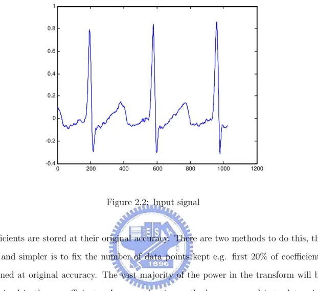
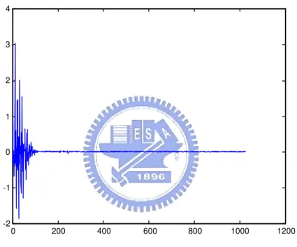
Orthogonal transforms provide alternate signal representations that can be useful for ECG data compression. Fig. 2.2, show an input signal with a sampling rate of 977 points/second and in Fig. 2.3 the discrete cosine transform of an electrocardiogram signal is given; it is clear from this diagram that the majority of the power in the transform is generally contained within the first 100 of the 1024 coefficients. Although a compression ratio of 10 : 1 with very little distortion might seem possible, this is not the case. The compression algorithm must also determine a threshold for how many

0 200 400 600 800 1000 1200 -0.4 -0.2 0 0.2 0.4 0.6 0.8 1

Figure 2.2: Input signal

coefficients are stored at their original accuracy. There are two methods to do this, the first and simpler is to fix the number of data points kept e.g. first 20% of coefficients retained at original accuracy. The vast majority of the power in the transform will be contained in these coefficients. A more adaptive method we proposed is to determine the upper bound in the spectrum and use it as the threshold to keep the coefficients that contain the vast majority of the power.

0 200 400 600 800 1000 1200 -2 -1 0 1 2 3 4

Chapter 3

Joint Turbo Source and Channel

Coding

It is well known that data compression and data transmission are essentially dual problems. In compression we remove all the redundancy in the data to form the most compressed version possible-the focus of source coding-whereas in transmission over noisy channels we add redundancy in a controlled fashion to combat errors in the channel-the purpose of channel coding. In channel-the past decade a series of research breakthroughs in the field of channel coding (most notably [11]), have rendered a large number of coding schemes which can achieve near-to-optimal performance (i.e. very close to channel capacity) with reasonable complexity. The secret of their success lies in the use of a ’turbo’ feedback in an iterative decoding scheme, an ingenious approach we call the ’turbo principle’ [12]. More recently, the turbo principle has been applied successfully to data compression of binary memoryless sources [13]. While in [14] the objective is to improve the error correction after transmission over a channel and therefore all encoded bits are useful, in the dual source coding problem addressed in [13] there is no channel involved and so the encoded bits can be punctured heavily depending on the desired compression rate. An alternative scheme based on LDPC codes and belief propagation decoding was presented in [1].

3.1

Decremental Redundancy–Source Coding

Let U be a binary, memoryless source drawn i.i.d. with p0 = P (U = 0). In this

section we describe how to encode a source block UN = (u1, · · · , un, · · · , uN) of length N

resulting in a binary codeword XK_{. We state how to generate this codeword in order to}

achieve compression on the one hand and protect the source information against channel impairments on the other hand. Our discussion can be expanded to any binary source. We use log-likelihood values with the natural logarithm throughout our discussion. For discrete model y = x + n, where y is the sample at the output of the received baseband matched filter, and x ∈ {0, 1} is the transmitted signal, we define the source state information (SSI) and the channel state information (CSI) by the two log-likelihood ratios LS = log p0 1 − p0, L(y|x) = log p(y|x = 0) p(y|x = 1) = LC · y

LC = 4Es/N0 for an additive white Gaussian noise (AWGN) channel and it is either ∞

or 0 for the binary erasure channel (BEC). In turbo source coding we successively remove the redundancy of a source sequence to obtain its most compressed representation. As long as the rate of the source code, defined as Rs = K_N, is larger than the entropy of the

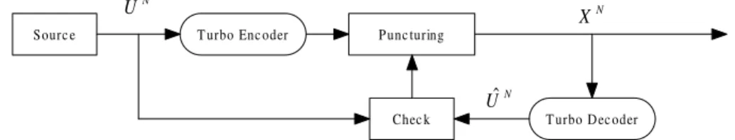
source H(U ), the source block can be perfectly reconstructed (source coding theorem). The proposed source coding scheme is based on the idea shown in Fig. 3.1. We

Source Turbo Encoder Puncturing

Check Turbo Decoder

N

Uˆ

N

U _XN

Figure 3.1: Lossless compression of a source block using turbo codes. Compression is achieved by puncturing and verifying the integrity of the reconstructed source sequence.

briefly explain its operation in the following. Further details are shown in [4]. The task of turbo compression is to map a source sequence UN _{to the compressed sequence X}K_.

The decremental redundancy algorithm encodes a source block of a binary memoryless source using a parallel concatenated (PCC) turbo code. The constituent codes of the turbo code are rate one convolutional codes (or scramblers). The PCC coding scheme is depicted in Fig. 3.2 As stated in [3] compression should be achieved by randomly

N U CC CC Puncture Puncture M U X P1N P2N P1K /2 P2K /2 XK

Figure 3.2: A parallel concatenation of rate 1 convolutional codes (CC) with an in-terleaver between them followed by heavy puncturing can be used to perform data compression of binary sources.

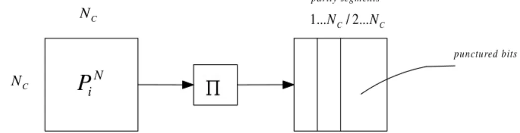
puncturing the scrambled (resp. parity) bits. In order to recover the source sequence perfectly, the randomly chosen puncturing pattern has to be saved. Accordingly, the side information is as long as the source block and thus compression is not possible. Hagenauer et al. [4] proposed this equivalent puncturing strategy depicted in Fig. 3.3

C N C N N i

P

parity segments C C N N /2... ... 1 punctured bits

Figure 3.3: Puncturing scheme for decremental redundancy.

Each parity sequence is interleaved, written line by line into a square matrix and the bits are erased columnwise. The decremental redundancy algorithm for turbo source encoding, which has the following steps:

2. Encode the source block with a turbo encoder and store the output block. 3. Puncture the encoded block using i parity segments.

4. Decode the compressed block.

5. Check for errors. If the decoded block is error free, let i = i + 1 and go to step 3. 6. Let i = i − 1. Repeat 3, include a binary codeword corresponding to the index i,

and stop.

Notice that the number of iterations required to find the best puncturing rate can be con-siderably reduced, if we store a table with different starting points for the optimization algorithm, depending on the probability distribution of the source. Since the sequences produced by the source are likely to be typical the number of iterations required to fine tune the compression rate will in general be small. We can also turn to a more sophisticated segmentation of the parity matrix, depending on the desired puncturing step.

Consequently, only the index of the last punctured column has to be known to reconstruct the source block. Since at least half of the parity bits have to be erased (otherwise we would have no compression) only dlog2(

√

N /2)e bits have to be stored as side information to indicate the size of the actual codeword. Finally, the compressed codeword XK _{is decoded using a parallel concatenated turbo decoder, resulting in the}

recovered source sequence ˆUN_{. As long as the reconstructed sequence is identical to the}

source sequence, we further can remove redundancy. If the integrity test fails for the first time, the index of the last cancelled column is incremented by one, and the resulting non-punctured parity bit constitute the compressed data.

Further on, we have to remark that each APP decoder is modified in order to benefit from the source statistics of the non-uniformly distributed binary source. In duality to the channel state information in channel coding, this additional input to the decoder

is called source state information. Thus APP component decoder is fed with the log-likelihood ratio LC· y, source state information LS and a priori information LA from the

other component decoder. In turbo compression the communication channel is BEC.

3.2

Source Decoding

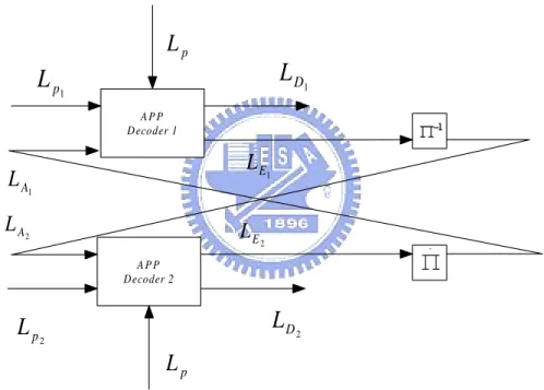
At first glance, random puncturing of bits does not seem to be a very sophisticated way of performing source compression. However, just as in channel coding with turbo codes, the sophisticated part lies in the use of a turbo decoder. The turbo decoder for our system is depicted in Fig. 3.4 We will use L-values to describe the values input

APP Decoder 1 APP Decoder 2 1 p

L

2 p

L

1 D

L

2 D

L

1 A

L

2 A

L

1 E

L

2 E

L

p

L

p

L

Figure 3.4: Parallel turbo source decoder.

and passed around by the turbo decoder. Given a binary random variable U , where for convenience u ∈ +1, −1, then the L-values is defined as,

L(U ) = loge

P (u = +1)

P (u = −1). (3.1)

More details on L-values can be found in [15]. In Fig. 3.4, LP₁, LP₂, LD₁, LD₂, LA₁, LA₂, LE₁, LE₂

”extrin-sic” respectively. Since the parity bit sequences P₁K/2 and P₂K/2 can be thought of as being ”transmitted” through a binary erasure channel (i.e. punctured), the correspond-ing input sequences LP1 and LP2 take on the L-values ±∞ (perfectly known bits) or 0 (erased).

In the case of a non-uniform binary source with P (U = +1) = p and P (U = −1) = 1 − p, for which H(U) = Hb(p) ((i.e. the binary entropy function), each decoder has an

additional input vector LP, where each element of the vector is equal to Lp = loge_1−pp .

We call this ’source’ apriori knowledge and distinguish between apriori knowledge which is learnt during the iterations of the decoder which we will call ’learnt’ apriori knowledge. In the case of more sophisticated (Markov) source models our source apriori vector would contain different sets of Lp values. The decoding algorithm is carried out according to

Fig. 3.4. APP decoder 1 uses LP1 and LA1 (initialized to zero in the first iteration) to calculate the extrinsic L-values LE1 = LD1− LA1− LP. The sequence LE1 is interleaved and passed onto APP decoder 2 as ‘learnt’ a priori knowledge LA2. Decoder 2 performs analogous operations and the process is then ”iterated” until convergence is achieved.

3.3

Designing the Puncture Table: A Dual of

Un-equal Error Protection

In some analogue source coding applications, like speech or video compression, the sensitivity of the source decoder to errors in the coded symbols is typically not uniform: the quality of the reconstructed analogue signal is rather insensitive to errors affecting certain classes of symbols, while it degrades sharply when errors affect other classes. We assume that the source encoder produces frames of binary symbols. Each frame can be partitioned into classes of symbols of different ‘importance’ (i.e. of different sensitivity). Each importance class is associated to its bit error rate (BER) requirement. For fixed code rate, decoding delay and complexity, it is apparent that the best coding strategy, called unequal error protection (UEP) aims at achieving lower BER levels

for the important classes while admitting higher BER levels for the unimportant ones. On the contrary, codes for which BER is (almost) independent of the position of the information symbols, are referred to as equal error protection (EEP) codes.

Turbo codes with UEP: Usually, turbo codes are punctured by using uniform punc-turing patterns. In the following section we show that this approach leads to EEP turbo codes. Suppose now that the information symbols in U are partitioned into c classes, according to some importance criterion, and let kl, denote the size of each class.

Without loss of generality, we enumerate the classes in non-decreasing importance or-der. Moreover, we assume k1 < k2 < · · · < kc, as in usual speech and video coding

applications. The intuitive idea for achieving UEP is as follows: we should increase the number of redundancy symbols correlated with the most important input symbols and reduce the redundancy correlated with the least important symbols, while keeping the total redundancy constant. This will be obtained by matching the puncturing patterns to the interleaver.

Then UEP is accomplished as follows: (i) arrange the input symbols u by rows in a Nc× Nc array U and consider a row-column interleaver, since it allows a clear graphical

representation of the input symbols arrangement and of the puncturing patterns as Nc × Nc array, such that N = Nc2 where N is the block size. (ii) each lth importance

class is associated to a partial rate rl, denoted as the inverse of the average number

of turbo encoded output symbols per input symbol belonging to the lth class. (iii) Partition U into c disjoint sets Sl of positions (i, j) of size kl , each corresponding to

class l, respectively. (iv) finally, ∀l = 1, · · · , c, a puncturing pattern realising the partial rate rl is associated to the positions of Sl.

The choice of the position sets Sl, affects the UEP property of the resulting turbo

code. In general, Sl must be chosen in order to correlate the turbo encoded redundancy

symbols to the input symbols belonging to a class l.

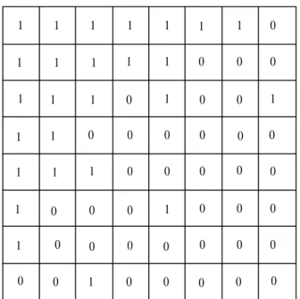
of the position subsets Sl is given in Table 3.1, where each position marked by l belongs to Sl for l = 1, 2, 3. 1 1 1 1 1 1 2 2 2 2 2 2 2 2 2 2 3 3 3 3 3 3 3 3 3 3 3 3 3 3 3 3 3 3 3 3 3 3 3 3 3 3 3 3 3 3 3 3 3 3 3 3 3 3 3 3 3 3 3 3 3 3 3 3

Table 3.1: Position subsets S1, S2, S3

For the EEP design case we use uniform puncturing on the whole set of redundancy symbols. For the UEP design case, Table 3.2 shows a choice for the puncturing pattern p1 (represented as a 13 × 13 binary array) which realises the partial rates for each class.

3.4

Upper Bounds of Discrete Cosine Transform

Application of fast discrete orthogonal transforms with various basis functions for data compression and efficient signal coding occupies a special place in the evolution of spectral representations. The digital spectral transform method is the main compres-sion tool in various signal and image processing applications. Particularly, the discrete cosine transform (DCT) based compression algorithms have become industry standard (JPEG, MPEG) for still and video image compression systems. The following basic lemma supplies a method for computing the exact values of the upper bounds of

spec-1 1 1 1 1 1 1 1 1 1 1 1 1 1 1 0 0 0 0 0 0 0 0 0 0 0 0 0 0 0 0 0 0 0 0 0 0 0 0 0 0 0 0 0 0 0 0 0 0 0 0 0 1 1 1 1 1 1 1 1 0 1 1 1

Table 3.2: Puncturing pattern p1 for UEP code

tral coefficients’ moduli on the class ω∆ [16] where

ω∆= {−→x = (x0, x1, · · · , xN −1) : max

1≤i≤N−1|xi−1− xi| ≤ ∆}, ∆ > 0. (3.2)

where ~x is the data vector.

Lemma 1 Let W =k ωj(i) kN −1j,i=0 be the matrix of a real-value discrete orthogonal

trans-form that satisfies the condition:

N −1 X i=0 ωj(i) = 0, j = 1, 2, · · · , N − 1, (3.3) and −→y = W −→x = (y0, · · · , yN −1)T. Then max x∈ω∆|y j| = ∆ · N −1 X m=1 ¯ ¯ ¯ ¯ ¯ m−1 X i=0 ωj(i) ¯ ¯ ¯ ¯ ¯ , j = 1, 2, · · · , N − 1. (3.4)

The proof of this lemma is based on the known dynamic programming principle [17], that is the initial extremal task is being broken down into a multiple-step process and the extremum being sought at each step according to the optimally principle. Note, that conditions (3.3) are satisfied for most of classical trigonometric, Walsh, as well as

Haar transforms [16]. On the other hand the relationship (3.4) remains true without conditions (3.3) if we put ω∆ instead of ω∆, where ω∆= −→x ∈ ω∆, x0 = 0

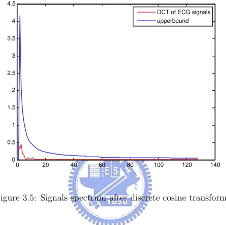
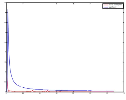
In Fig. 3.5 the absolute value of DCT of an signal and it’s DCT upper bound are

0 20 40 60 80 100 120 140 0 0.5 1 1.5 2 2.5 3 3.5 4 4.5 DCT of ECG signals upperbound

Figure 3.5: Signals spectrum after discrete cosine transform.

given. By Fig. 3.5, we can set the threshold to keep the coefficients that contain the vast majority of the power in the spectrum.

But in some cases, as in Fig. 3.6 the threshold may not so good in keeping the vast majority of the power in the spectrum. So we must use the UEP’s idea to divide the different parts of the spectrum into different classes.

3.5

Joint Source and Channel Coding Using

Un-equal Protection

In this section, we present a joint source and channel coding method for electrocar-diogram (ECG) signals based on transform data and unequal protection. This proposed compression scheme may find applications in digital Holter recording, in ECG signal

0 20 40 60 80 100 120 140 0 0.5 1 1.5 2 2.5 3 3.5 4 4.5 DCT of ECG signals upperbound

Figure 3.6: Signals spectrum after discrete cosine transform.

archiving and in ECG data transmission through communication channels. Using the new method, a compression ratio of 10 to 1 can be achieved with P RD = 3.8%, in contrast to the AZTEC compression ratio of 6.8 to 1 with P RD = 10.0% , the fan algo-rithm compression ratio of 7.4 to 1 with P RD = 8.7%, and symmetric wavelet transform compression ratio of 8 to 1 with P RD = 3.9%.

A turbo ECG compression system is shown in Fig. 3.7. The signal is first divided into

Blocking Transform Quantizer _EncoderTurbo Compressor Upper Bound computer Design Puncturing table Turbo Decoder Integrity Check x c uˆ u input T urbo compression

segments of n samples by a blocking algorithm. The segments are transformed using a Direct Cosine Transform. The upper bound computer determines the ∆ in each blocks. Based on the ∆, the puncturing table could be designed by our puncturing scheme. The turbo compression scheme efficiently codes the output in the form of compressed data.

Detailed operations of each block are described below.

Blocking: The size of segmentation is important in determining the compression ratio and the distortion amplitude. A large number of points in a segment tends to increase the maximum of the upper bound, it makes the upper bound unreliable. We experimented with several segment sizes. For most ECG tapes, a block size of 1024 samples (1 seconds of record, about 2 normal beats) is appropriate.

Block size is an important issue about the system complexity. We used the discrete cosine transform to implement the transform block. So O(N logN ) operations are needed for block size N of DCT. We choose N as small as possible to reduce the complexity of system. But the block size must keep the idea of transform method, it should have more than one normal beat period (about 350 to 450 samples).

The performance of turbo code is effected by some factors, such as constrain length, iteration number, the size of interleaver, the category of interleaver ,and so on. The constrain length is usually 3 ∼ 5. Too large constrain length will increase the necessary decoding time and the complexity of decoding, but the improved effect of performance is limited. Here we will not discuss the influence of constrain length and iteration on the performance of turbo code. we only discuss on the effects of interleaver block size.

• Memory : Memory usage(interleaver size, extrinsic information registers, operation registers, · · · ) is directly proportion to the block size. So, the block size is choosed as small as possible to reduce the memory usage.

• Processing Time : The puncture scheme we proposed shows that decoding time is directly proportion to the block size, because of the turbo decoder’s iteration

times. So, the block size is choosed as small as possible to reduce the processing time.

• Performance : The greater block size N represents the better performance of turbo code. However, the drawback of great size is that increase the necessary of decoding time.

Transform: We used the discrete cosine transform to implement the transform block.

Upper bound computer: This is an important operation in the system. The number of bits assigned to the puncturing table is inversely proportional to the distortion at the reconstructed output. The objective is to count the best threshold to minimize the puncturing table’s bit.

Quantizer: The quantizers is designed to uniformly round up the decomposed signals into integer values. Although a non-uniform quantizer will reduce the rate of distortion, it will cause a significant peak amplitude variation of the QRS complexes in the ECG signal.

Design Puncturing Table: In a first step the parity bits in each block PN

i with i =

1, 2 are written line by line in a matrix Nc×Nc, such that N = Nc2, where N is the block

size. since it allows a clear graphical representation of the input symbols arrangement and of the puncturing patterns. Second, based on the output from transform, a good selection of the position subsets S, is given in Table 3.3 , where each position marked by 1 belongs to Sl, for l = 1, 2, 3.

Third, based on the upper bound’s output, we design the puncturing table could that achieve the compression rate desired shown in Table 3.4. To gradually remove the redundancy in the encoded stream we can eliminate one such parity segment at a time (in parallel for PN

1 and P2N ), yielding a puncturing step of 2Nc/N that allows us to

fine tune the compression rate. To make sure that the erased bits are spread out in the block we interleave the parity bits before puncturing them.

1 1 1 1 1 1 2 2 2 2 2 2 3 3 3 3 3 3 3 3 3 3 3 3 3 3 3 3 3 3 3 3 3 3 3 3 3 3 3 3 3 3 3 3 3 3 3 3 3 3 3 3 1 2 1 1 1 1 1 1 1 2 2 2

Table 3.3: Position subsets

Turbo compression: Turbo encoder is shown in Fig. 3.8. The only difference between traditional turbo code is our encoder without having the systemic part. The key idea of lossless compression is the puncturing table we proposed . We propose the decremental redundancy scheme illustrated in Fig. 3.4. The reconstructed source sequence is compared with the original block at the encoder side and the puncturing rate is adjusted to the result of this integrity test. This rate is decreased if the integrity test fails and vice versa. Puncturing , decoding, the check for integrity and rate adjustment defined as one cycle of the analysis by synthesis (AbS) loop. In each successful AbS loop, it depends on the convergence of the decoding algorithm which means we puncture less bits than it can be corrected by the chosen turbo code. Clearly, without convergence of the decoding result the source information cannot be perfectly recovered. To guarantee that the decoder is able to decode the input sequence without errors (lossless source coding), we can enable the encoder to test the decodability of its output. Since we want to achieve as much compression as possible, we puncture the parity bits on a step by step basis (decremental redundancy) as long as the compressed block can still be

1 1 1 1 1 1 1 1 1 1 1 1 1 1 1 0 0 0 0 0 0 0 0 0 0 0 0 0 0 0 0 0 0 0 0 0 0 0 0 0 0 0 0 0 0 0 0 0 0 0 0 0 1 1 1 0 0 0 0 0 0 0 0 0

Table 3.4: Puncturing pattern based on the upper bound computer, for UEP code

decoded error free by the test decoder at the source compression side. We now proceed to describe our decremental redundancy algorithm for turbo source encoding, which has the following steps:

1. Let i = Nc/2.

2. Encode the source block with an encoder based on turbo principle and store the output block.

3. Puncture the encoded block using the idea of UEP. 4. Decode the compressed block.

5. Check for errors. If the decoded block is error free, let i = i − 1 and go back to step 3.

6. Let i = i + 1. Repeat step 3, include a binary codeword corresponding to the index i , and stop.

M essage bits Flip-Flop M odulo-2 adder Parity-check bits Parity-check bits

Figure 3.8: Block diagram of turbo-principle-based encoder

3.5.1

Simulation Results

The turbo compression method was applied to the ECG signal and transmit through Additive White Gaussian Noise (AWGN) channel. The results show the high efficiency of this method for ECG compression. The original signal, reconstructed signal and error between them for three records with the corresponding CR and PRD values are shown in Fig.3.9.

The compression ratios and the percent root-mean-square differences are tabulated below for the proposed method. Although the percent root-mean-square difference does not account for differences between morphology of two signals an may not report shape distortions, is used widely in signal compression literature as a standard measurement, because it is easy to compute and compare. Compression ratio (CR) is computed from the ratio of the original signals’ samples (in bits) to the length of output bit stream. By

0 200 400 600 800 1000 1200 −0.5 0 0.5 1 time(ms) voltage Original Signal 0 200 400 600 800 1000 1200 −0.5 0 0.5 1 time(ms) voltage Reconstructed Signal, CR = 10.3 , PRD= 0.0(%) 0 200 400 600 800 1000 1200 −1 −0.5 0 0.5 1 time(ms) voltage Error

Figure 3.9: Compression with joint turbo source and channel coding

this method, we achieved the compression ratio about 10 with lossless data compression. Also , in table 3.5 is given the CR and PRD values for some other compression methods. In Fig. 3.10, it shows that the proposed method has lower average PRD through an AWGN channel. The SN Ro defined as the ratio of the average power of the message signal (before compression) to the average power of the noise, both measured at the receiver output.

Compression method Compression ratio PRD (%) AZTEC[6] 6.8 10.0% TP[7] 2.0 5.3% CORTES[8] 4.8 7.0% Fan/SAPA[10] 3.0 4.0% Symmetric Wavelet 7.9 3.9% Proposed method 10.0 0.0%

Table 3.5: Compression performance for ECG signals with different compression method

-5 -4 -3 -2 -1 0 1 2 3 0 20 40 60 80 100 PRD (%) SNRo(dB) proposed method

wavelet +arithmetic + turbo code

Figure 3.10: Average PRD comparison between proposed method and wavelet transform with arithmetic coding and rate-1/2 turbo coding

Chapter 4

Adaptive Multirate Approach for

Electrocardiogram Compression

By inspection, there is an apparent similarity between speech and the nature of ECG signals, which indicates a possible application of speech coding technology to ECG data compression. There can be a large variance amongst different ECG’s, reminiscent of that found in human speech. The importance of details in different rhythms varies over various applications while the ultimate goal is a coding algorithm that faithfully reproduces original signals.

The AMR-WB speech codec algorithm was selected in December 2000 and the corre-sponding specifications were approved in March 2001. The AMR-WB codec was also se-lected by the International Telecommunication Union-Telecommunication Sector (ITU-T) in July 2001 in the standardization activity for wideband speech coding around 16 kb/s and was approved in January 2002 as Recommendation G.722.2.

With the ultimate aim of using the idea of Adaptive Multi-Rate Wideband speech codec, the present thesis is structured as follows. The following section reviews the the-oretical background of linear prediction and introduces the basic concepts of analysis-by-synthesis based linear predictive coders, the general class to which the Code-Excited Linear Prediction [18] coding algorithm belongs. Pitch prediction techniques and code-book constructed methods are also discussed.

4.1

The Code Excited Linear Prediction Coder

The proposed coder is based on the code excited linear prediction coder (CELP) structure for signal compression. CELP is a parametric coder; the basic parts comprise an excitation signal drawn from a codebook (a collection of codevectors) and shaped through a long term predictor and an AR filter (LPC model), synthesizing the output signal. The parameters are calculated in an analysis-by-synthesis fashion: the long-term and short-term filters ( l/P (z) and l/A(z)) are determined from the incoming signal, and the best codevector (in an MSE sense) is found through filtering, comparison, and selection.

The basic CELP is shown in Fig.4.1. Parameters from coding are the LPC coeffi-cients ({ak}), the long-term prediction lag and gain coefficient (D, β), and the codebook

index (i). A(z) LPC analysis Long-term prediction 1/P(z) 1/A(z) codebook Minimisation incoming signal k

a

gain index lag gain

Figure 4.1: CELP coder

4.1.1

Linear Prediction Analysis

One of the most powerful speech analysis techniques is based on linear prediction. This method has become the predominant technique for estimating the basic speech

parameters such as the fundamental frequency F0, vocal tract area functions, and the

frequencies and bandwidth of spectral poles and zeros (e.g formants), and for repre-senting speech for low bit rate transmission. The basic idea in linear prediction is that a speech sample is approximated as a linear combination of past speech samples. By minimizing the sum of the squared difference (over a finite interval) between the actual speech samples and the linearly predicted ones, a unique set of predictor coefficients can be determined. For speech, the prediction is done most conveniently in two separate stages: a first prediction based on the short-time spectral envelope of speech known as short-term prediction, and a second prediction based on the periodic nature of the spectral fine structure known as long-term prediction. So , for ECG signals, the same we divide it into two stages: long-term prediction and short-term prediction.

The short-term linear prediction analysis in Fig. 4.2 estimates the all pole filter in each frame, used to generate the spectral envelope of speech signal. The filter typically has 10 − 12 coefficients. We have used MATLAB’s lpc function to obtain these coeffi-cients however they can be obtained by implementing a lattice filter which acts both as a forward and backward error prediction filter. It gives us reflection coefficients which can be converted to filter coefficients. Levinson-Durbin method can be used effectively to reduce complexity of the filter.

ˆ s(n) = p X i=1 ais(n − i) (4.1)

The error between the actual value s(n) and the predicted value ˆs(n) is given by: r(n) = s(n) − ˆs(n) = s(n) −

p

X

i=1

ais(n − i) (4.2)

The error,r(n) , is also known as the formant residual signal. Taking the z-transform on both sides, Eq. 4.2 can be written as:

R(z) = S(z)[1 −

p

X

i=1

A signal production model can be defined, where an excitation signal E(z) is passed through a shaping filter,

H(z) = 1

1 −Pp

i=1aiz−i

(4.4) to produce the reconstructed signal ˆS(z). H(z) is the formant synthesis filter and can be interpreted as the frequency response of the vocal tract. A(z) expressed as

A(z) = 1 −

p

X

i=1

aiz−i = 1 − F (z) (4.5)

is the inverse formant filter; its main function is to remove the formants structure from the original signal file.

) (n s

)

(

ˆ n

s

)

(n

r

Figure 4.2: Formant prediction.

Linear prediction is optimal in the least-squares sense if the samples of the signal are assumed to be random variables with Gaussian distribution. Experiments have shown that, taken over short time segments, signal samples can be assumed to have a Gaussian distribution. If the prediction system is based on past original samples, we refer to it as forward adapted prediction because the predictor coefficients have to be sent to the receiver as side information. However, if the prediction system is based on past reconstructed samples, we refer to it as backward adaptive prediction and no side information is transmitted because the predictor coefficients can be calculated both at the transmitter and the receiver.

The least-squares method is used in order to determine the Linear Prediction Coefficients (LPC) and is based on minimizing the total squared error with respect to

each of the parameters. However, the signal s(n) is not stationary and its statistics are not explicitly known, so it is common practice to consider the ECG signal as stationary over short time intervals.

The residual signal from the formant analysis filter, A(z), still shows pitch peri-odicity. Another important feature in linear predictive coders is to remove the far-sample redundancy from the original signal. Pitch prediction can be handled by a filter with

) (n r

)

(

ˆ n

r

)

(n

e

Figure 4.3: Pitch prediction

only one coefficient of the following form:

P (z) = βz−D _(4.6)

where β is a scaling factor related to the degree of waveform periodicity and D is the estimated period in samples. This predictor has a time response of a unit sample delayed by M samples; so the pitch predictor estimates that the previous pitch period repeats itself. ECG signals have a pitch in a few hundred hertz. In our implementation we consider pitch frequencies from 350Hz to 450Hz. For 1kHz signal these frequencies correspond to pitch delay of 350 samples to 450 samples. For ECG signals, the excitation sequence shows a significant correlation from one pitch period to the next. Therefore, a long-delay correlation filter is used to generate the pitch periodicity in ECG signals as shown in Fig. 4.3. The error signal is

and is called the pitch residual signal. Taking the z-transform on both sides, and rear-ranging the terms, the inverse pitch filter is defined to be

B(z) = 1 − βz−D _(4.8)

Its main function is to remove the pitch structure from the original signal. At the decoder stage, the pitch synthesis filter defined as

G(z) = 1

1 − P (z) (4.9)

is excited by the formant residual signal in order to introduce a periodic structure, matching as close as possible that of the original signal.

4.1.2

Line Spectral Frequencies

In order to increase the compression rate, we need to quantize the coefficients using the less bits as possible as we can. It causes the unstability of the filter, so we have used MATLAB’s poly2lsf function to convert prediction filter coefficients to line spectral frequencies. Line Spectral Frequencies (LSF) is a very popular set for representing the LPC coefficients, because they are related to the speech spectrum characteristics in a straightforward way. The LSF represents the phase angles of an ordered set of poles on the unit circle that describes the spectral shape of the inverse formant filter A(z) defined in Eq.?? They were first introduced by Itakura in 1975 [19] The main advantages of the LSF are that they can provide easy stability checking procedures, spectral manipulations, and convenient re-conversion to predictor coefficients.

Conversion of the LPC coefficients ak to the LSF domain relies on the inverse

formant filter A(z). Given A(z), its corresponding LSF are defined to be the zeros of the polynomials P (z) and Q(z) defines as :

A(z) = 1 + p X k=1 akz−k (4.10) P (z) = A(z) − z−(p+1)_A(z−1_{) (4.11)} Q(z) = A(z) + z−(p+1)_A(z−1_{) (4.12)}

so (4.11) and (4.12) become P (z) = (1 − z)(A0zp+ A1zp−1+ · · · + Ap) (4.13) Q(z) = (1 + z)(B0zp+ B1zp−1+ · · · + Bp) (4.14) where A0 = 1 B0 = 1 Ak = (ak− ap+1−k) + Ak−1 (4.15) Bk = (ak+ ap+1−k) + Bk−1 (4.16)

where k = 1, 2, · · · , p in (4.13) and (4.14) (1 − z) and (1 + z) are known, so we only need to consider

P0_{(z) = A}

0zp+ A1zp−1+ · · · + Ap (4.17)

Q0_{(z) = B}

0zp+ B1zp−1+ · · · + Bp (4.18)

using z-transform to transform (4.17) and (4.18) into P0_{(z) = z}p_2[A 0(z p 2 + z−p2 ) + A₁(z p 2−1+ z −p 2 +1) + · · · + Ap 2] (4.19) Q0_{(z) = z}p_2[B 0(z p 2 + z−p2 ) + B₁(z p 2−1+ z−p2 +1) + · · · + Bp 2] (4.20)

If A(z) is minimum phase, all the roots of P (z) and Q(z) will lie on the unit circle, alternating between the two polynomials with increasing frequency. The roots occur in complex conjugate pairs and hence there are p LSF lying between 0 and π. The value of the LSF can be converted to Hertz (Hz) by multiplying by the factor Fs/2/pi where

Fs is the sampling frequency. Another important characteristic about the LSF is the

localized spectral sensitivity. For the predictor coefficients, a small distortion in one coefficient could dramatically distort the spectral shape and even lead to an unstable synthesis filter. Whereas, if one the LSF is distorted, the spectral distortion occurs only

in the neighborhood of the modified LSF.

In many LPC coders, the LPC filtering is carried out by interpolating the predictor coefficients between two successive analysis frames into a subframe level such that a smoother transition is achieved. The interpolation can be performed in the LSF domain to guarantee the stability of the resulting filters.

4.1.3

Codebook Generation

Vector Quantization (VQ) [20] has been widely known for its excellent rate-distortion performance. It may be simply viewed as a form of pattern recognition or matching where an input pattern is ‘approximated’ by one standard template of a predetermined codebook. Conceivably, a good vector quantizer is subject to a good codebook. The most commonly used method for designing a VQ codebook is the LBG algorithm [20]. It is an iterative method and involves creating a primitive seed of letter reference from which an improving alphabet evolves step by step. The performance of the overall codebook depends on the selection of the initial seed (codebook). This initial seed could be a code generated arbitrarily or adopted previously. Nevertheless, the almost exclusively adopted method is called the splitting algorithm[20], which grows increasingly larger codebooks of a fixed dimension from the lowest resolution codebook of a training set to the codebook of size as required for the initial seed. And, the simplest but less reliable initialization is by means of the so-called random guess method [20].

In 1980, Linde, Buzo, and Gray (LBG) proposed a VQ design algorithm based on a training sequence. The use of a training sequence bypasses the need for multi-dimensional integration. A VQ that is designed using this algorithm are referred to in the literature as an LBG-VQ. A VQ is nothing more than an approximator. The idea is similar to that of “rounding-off” (say to the nearest integer). An example of a 1-dimensional VQ is shown in Fig.4.4: Here, every number less than -2 are approximated by -3. Every number between -2 and 0 are approximated by -1. Every number between

Figure 4.4: One dimensional VQ

0 and 2 are approximated by +1. Every number greater than 2 are approximated by +3. Note that the approximate values are uniquely represented by 2 bits. This is a 1-dimensional, 2-bit VQ. It has a rate of 2 bits/dimension. An example of a 2-dimensional VQ is shown in Fig.4.5: Here, every pair of numbers falling in a particular region are

Figure 4.5: Two dimensional VQ

and 16 red stars–each of which can be uniquely represented by 4 bits. Thus, this is a 2-dimensional, 4-bit VQ. Its rate is also 2 bits/dimension. In the above two examples, the red stars are called codevectors and the regions defined by the blue borders are called encoding regions. The set of all codevectors is called the codebook and the set of all encoding regions is called the partition of the space.

We assume that there is a training sequence consisting of M source vectors: τ = {x1, x2, · · · , xM}. This training sequence can be obtained from some large database. For

example, if the source is a speech signal, then the training sequence can be obtained by recording several long telephone conversations. M is assumed to be sufficiently large so that all the statistical properties of the source are captured by the training sequence. We assume that the source vectors are k-dimensional, e.g. xm = (xm,1, xm,2, · · · , xm,k), where

m = 1, 2, · · · , M. Let N be the number of codevectors and let C = {c1, c2, · · · , cN},

represents the codebook. Each codevector is k-dimensional, e.g., cn = (cn,1, cn,2, · · · , cn,k)

where n = 1, 2, · · · , N. Let Snbe the encoding region associated with codevector cnand

let P = {S1, S2, · · · , SN} denote the partition of the space. If the source vector xm is in

the encoding region Sn, then its approximation (denoted by Q(xm)) is cn: Q(xm) = cn ,

if xm ∈ Sn. Assuming a squared-error distortion measure, the average distortion is given

by: Dave = 1 M k M X m=1 kxm− Q(xm)k2 (4.21)

LBG Design Algorithm is as follows:

1. Given τ . Fixed ² > 0 to be a small number. 2. Let N = 1 and c∗ 1 = 1 M M X m=1 xm. (4.22) Calculate D∗ ave = 1 M k M X m=1 kxm− c∗1k. (4.23)

3. Splitting: For i = 1, 2, · · · , N, set c0_i = (1 + ²)c∗ i (4.24) c0_{N +i = (1 − ²)c}∗ i (4.25) Set N = 2N 4. Iteration: D0

ave = Dave∗ . Set the iteration index i = 0

(a) For m = 1, 2, · · · , M, find the minimum value of

kxm− c(i)n k2, (4.26)

over all n = 1, 2, · · · , N. Let n∗ _{be the index which achieves the minimum.}

Set

Q(xm) = c(i)n . (4.27)

(b) For n = 1, 2, · · · , N , update the codevector ci+1_n = P Q(xm)=cinxm P Q(xm)=cin1 (4.28) (c) Set i = i + 1 (d) Calculate Di_ave = 1 M k M X m=1 kxm− Q(xm)k2 (4.29) (e) If Di−1

ave − Davei /Di−1ave > ², go back to Step 4a.

(f) Set D∗

ave = Diave. For n = 1, 2, · · · , N, set c∗n= cin as the final codevectors.