感知無線營運商之頻譜分享機制研究

I

國

立

交

通

大

學

網路工程研究所

碩

士

論

文

感知無線營運商之頻譜分享機制研究

The Study of Spectrum Sharing among Cognitive Radio Operators

研 究 生：林佳賢

指導教授：趙禧綠 教授

ii

感知無線營運商之頻譜分享機制研究

The Study of Spectrum Sharing among Cognitive Radio Operators

研 究 生：林佳賢 Student：Chia-Hsien Lin

指導教授：趙禧綠 Advisor：Hsi-Lu Chao

國 立 交 通 大 學

網 路 工 程 研 究 所

碩 士 論 文

A Thesis

Submitted to Institute of Network Engineering College of Computer Science

National Chiao Tung University in partial Fulfillment of the Requirements

for the Degree of Master

in

Computer Science

September 2012

Hsinchu, Taiwan, Republic of China

I

摘 要

無線感知與動態頻譜存取可以使無線用戶共享一個廣泛可用頻譜。在感知無線電網路，次 級用戶被允許存取主要用戶的通道。在本篇論文中，我們考慮通道分配問題在給定的條件限制 下，針對網路運營商之間，在感知無線電網路中達到最大通道分配之吞吐量。接著我們也考慮 可用的通道中的主要用戶的行為，這些可用的通道一次只能分配給一個運營商，然後我們將我 們的問題對應到 0-1 多個背包問題，並將此問題修改成符合我們所求的條件。 更進一步，我們設計了兩演算法來解決這個問題並將模擬結果表現出來。在第一個演算法 中，我們設計出這個演算法可以非常接近最大的吞吐量。在第二個演算法中，我們設計出這個 演算法可以大大的降低此問題排程的時間複雜度。最後，模擬結果表現出我們所提出來的方法 可以很接近此問題的最佳解。

II

Abstract

Cognitive radio and Dynamic Spectrum Access (DSA) enable wireless users to share a wide range of available spectra. In cognitive radio networks, secondary users are allowed to access the channels licensed to primary users. In this thesis, we consider the channel assignment problem as a resource allocation problem under some constraints for throughput maximization in cognitive radio networks over network operators. We also consider the primary user activity on available channels where each operator can be allocated at most one available channel, then we formulate our problem as a 0-1 multiple knapsack problem (0-1 MKP) which is a NP-hard problem but the constraint of our problem is different from the original problem.

Moreover, we design two algorithms to solve this problem and compare their performance in the simulation results. From the simulation results, we demonstrate that the first designed algorithm achieves a high throughput performance, while with high complexity. On the other hand, the proposed second algorithm aims at significantly reducing the time complexity while it has only about 98% throughput performance, compared with the first algorithm.

III

致 謝

回想起當初進到研究所的時候，才從軍中退伍不久，加上對資訊科學與網路工程完全是個 門外漢，一切從零開始，研究所的課業、文獻的搜尋與閱讀都是我在大學期間完全沒接觸過的， 對我來說，這是一個全新的挑戰。 在研究所兩年期間，我要感謝我的指導教授--趙禧綠老師悉心的指導，不論在課業及未來 就業的方向，老師都提供了相當寶貴的意見，使得能夠在自己的人生道路上有完善的規劃，雖 然自己仍然多次的犯錯及表現不佳，老師仍不厭其煩的指導與協助，引領我一步一步前往正確 的方向。真的非常的感謝老師的教導。 接著要感謝實驗室的學長、學姐、同學以及學弟妹，在我遇到課業與論文的挫折時，給予 最大的支持與鼓勵。也感謝我的家人及好友，在我的求學道路上，陪我一起渡過這段艱辛的成 長與學習。最後感謝交大提供這麼棒的研究與教學資源，讓學生們都能很順利的取得最新且最 珍貴的學術資訊。

IV

CONTENT

摘 要... I ABSTRACT ... II 致 謝... III LIST OF FIGURE ... V LIST OF TABLES ... VI CHAPTER1. INTRODUCTION ... 1

1.1BACKGROUND OF COGNITIVE RADIO NETWORKS ... 1

1.2REVIEW OF RELATED STUDIES ... 1

1.3MOTIVATION AND OBJECTIVE ... 2

CHAPTER2. SYSTEM MODEL AND ASSUMPTIONS ... 4

2.1SYSTEM MODEL ... 4

2.2ASSUMPTIONS ... 4

CHAPTER3. PROBLEM FORMULATION ... 7

3.1PROBLEM MAPPING... 7

3.2PROBLEM FORMULATION ... 8

CHAPTER4. THE PROPOSED METHODS ... 9

4.1AN OPTIMIZATION SOLUTION OF THE OBJECTION FUNCTION ... 9

4.2ALGORITHM1:TOTAL EXCHANGE ALGORITHM ... 9

4.3ALGORITHM2:LEVEL EXCHANGE ALGORITHM ... 13

CHAPTER5. SIMULATION RESULTS... 17

5.1PARAMETER SETTING OF SIMULATIONS ... 17

5.2SIMULATION RESULTS ... 18

CHAPTER6. CONCLUSION AND FUTURE WORK ... 25

V

List of Figure

Figure 1: System Model ... 4

Figure 2: The sum of channel capacity of three methods at different scenarios when ... 19

Figure 3: The percentage of two methods compare to brute-force at three scenarios when ... 19

Figure 4: The sum of channel capacity of three methods at different scenarios when ... 20

Figure 5: The percentage of two methods compare to brute-force at three scenarios when ... 20

Figure 6: The sum of channel capacity of three methods at different scenarios when ... 21

Figure 7: The percentage of two methods compare to brute-force at three scenarios when .. 22

Figure 8: The sum of channel capacity of three methods at different in the Scenario 1 ... 23

Figure 9: The sum of channel capacity of three methods at different in the Scenario 2 ... 23

VI

List of Tables

Table 1: A list of notations... 5

Table 2: Mapping Table. ... 7

Table 3: Algorithm1 pseudo code ... 9

Table 4: Channel allocation of Algorithm1 ... 10

Table 5: Channel Exchange of Algorithm1 ... 11

Table 6: The detail of channel exchange in Channel Exchange of Algorithm1 ... 12

Table 7: Algorithm2 pseudo code ... 13

Table 8: Channel Allocation of Algorithm2 ... 14

Table 9: Channel Exchange of Algorithm2 ... 15

Table 10: Simulations and analysis parameters ... 17

1

Chapter1. Introduction

1.1 Background of Cognitive Radio networks

Current wireless networks are characterized by a static spectrum allocation policy, where governmental agencies assign wireless spectrum to license holders on a long-term basis for large geographical regions. The Federal Communications Commission (FCC) [1] assigns spectrum to licensed holders, also known as primary users. Recently, because of the increase in spectrum demand, this policy faces spectrum scarcity in particular spectrum bands. The inefficient usage of the limited spectrum necessitates the development of dynamic spectrum access techniques, where users who have no spectrum licenses, also known as secondary users, are allowed to use the temporarily unused licensed spectrum. Hence, dynamic spectrum access (DSA) techniques were recently proposed to solve these spectrum inefficiency problems. The key enabling technology of dynamic spectrum access techniques is cognitive radio technology [2]. DSA is proposed to solve these current spectrum inefficiency problems. However, spectrum sharing between primary users and secondary users brings us into a great challenge that the secondary users’ activity may cause severe interference with the primary users. Secondary users may occupy available bands as long as the corresponding primary user is not active, but must immediately evacuate the band as soon as the corresponding primary user appears [3]. The frequency spectrum can be shared among primary users and secondary users to improve spectrum utilization.

1.2 Review of Related Studies

One of classification for spectrum sharing [3] between primary users and secondary users in Cognitive networks is based on the access technology is overlay and underlay spectrum sharing mode. Wherein secondary users should stop transmission on the channel once primary users are detected is called overlay mode [8, 10]. In [8, 10] define a throughput metric to decide to allocate channel to secondary users, these two papers’ main ideal of proposed methods is greedy to assign resource depends on factor which is predefined. And wherein secondary users and primary users can coexist and share the same spectrum with each other in case the interference caused by secondary

2

users is under the predefined threshold is called underlay mode [11 - 16]. In [11 - 16], those papers’ problem have the same action that is mapping the problems to a non-linear integer programming or a binary integer optimal programming and adding some constraint, such as power constraint, interference constraint, then they proposed a greedy heuristic algorithm to solve those problems. In this thesis, we want to use overlay mode to model our problem, because we model this problem using operators’ view that don’t consider primary users’ interference. Many of literature to solve sharing problem such as game theoretical analysis [4], auction-based theory [5], but these literature focus on primary users and secondary users to share the same bands. However, in this thesis, we concentrate on primary band to locate idle time to network operators in a fix time period. We proposed two algorithms to solve this resource allocation problem.

There are several research efforts on spectrum allocation in Cognitive radio technologies on the overlay mode. In the literature, some papers consider interference between primary users and secondary users with few SINR (signal- interference-plus-noise-ratio) constraints [8]. These papers constructed objective functions to maximize, with some conditions to mapping to problems that presented a mixed integer nonlinear programming (MINLP) optimization spectrum sharing model [6] or formulated a binary integer linear programming (BILP) model [7], trying to establish as many links between SUs as possible. Meanwhile, [9] put a suboptimal strategy for Cognitive Radio channel allocation, with the objective of maximizing the whole Cognitive Radio networks’ throughput. However, in [6], the MINLP model is an NP-hard problem and the solution algorithm complexity is relatively high.[7] never put any mathematic algorithm to solve its BILP model and had no standards to evaluate the performance of the solution solved by software LINGO. Most importantly, [6], [7], and [9] are not consider primary users activity, so these papers are not consider all of conditions which is one of the most important parameters in a cognitive radio networks.

1.3 Motivation and Objective

In Cognitive radio networks, primary users are not always using their own channel to communication, so secondary users can communication to other secondary users when the primary channel is vacated. First, we consider the operators’ traffic load which is collect by each operator of total transmission time that comes from secondary users’ data transmission time. Then, we assign channel to operators depends on operators’ traffic load and channel capacity. So, how to assign channels to operators is the crucial problem. This thesis will induce cloud computing architecture to

3

be our system model, which can help to assign channel from primary bands to operators. We solve the problem which is spectrum sharing among operators that is different from the related works which is spectrum sharing between primary users and secondary users. Then, the cloud servers execute algorithms which we proposed to satisfy each operator’s demand, and can be a low time complexity algorithm which will reach the optimal solution of objective function.

4

Chapter2. System Model and Assumptions

In this chapter, we will describe the system model; introduce the definitions of the assumptions caused by primary users’ channel, secondary users’ transmission time, operators’ traffic load, allocation time window, and some constraints.

2.1 System Model

The system model of our problem used in this thesis is illustrated in Figure 1, where there are some operators, several secondary users, and primary users. We split the secondary users into secondary transmitter and secondary receiver. Secondary transmitters transmit data on the channel. Secondary receivers are in the receiving mode, and can receive data from secondary transmitters.

Figure 1: System Model

2.2 Assumptions

There are two modes in Cognitive radio networks for spectrum sharing between secondary users and primary users. One mode is called underlay, wherein secondary users and primary users can

5

coexist and share the same spectrum with each other in case the interference caused by secondary users is under the predefined threshold, but in this thesis, we don’t consider this mode, because when primary user come back to use the band, we called busy period which the secondary users cannot transmission on this channel. The other one is called overlay, wherein secondary users should stop transmission on the channel once primary users are detected [11]. In this thesis, we focus on the overlay mode.

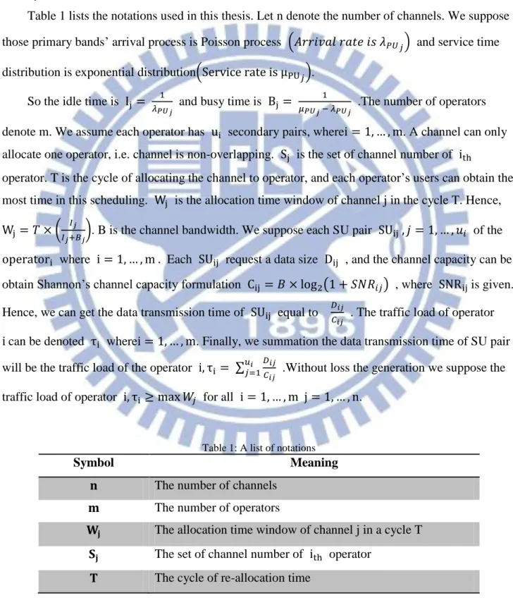
Table 1 lists the notations used in this thesis. Let n denote the number of channels. We suppose those primary bands’ arrival process is Poisson process ( ) and service time distribution is exponential distribution( ).

So the idle time is

and busy time is .The number of operators

denote m. We assume each operator has secondary pairs, where . A channel can only allocate one operator, i.e. channel is non-overlapping. is the set of channel number of

operator. T is the cycle of allocating the channel to operator, and each operator’s users can obtain the most time in this scheduling. is the allocation time window of channel j in the cycle T. Hence,

( ). B is the channel bandwidth. We suppose each SU pair of the where Each request a data size , and the channel capacity can be obtain Shannon’s channel capacity formulation ( ) , where is given. Hence, we can get the data transmission time of equal to

. The traffic load of operator

can be denoted where . Finally, we summation the data transmission time of SU pair will be the traffic load of the operator ∑

.Without loss the generation we suppose the

traffic load of operator for all .

Table 1: A list of notations

Symbol Meaning

The number of channels The number of operators

The allocation time window of channel j in a cycle T The set of channel number of operator

6

The primary user The secondary user

The secondary pair from operator to the SU j The data size from operator to the SU j

The channel capacity from operator to the SU j

The channel bandwidth

The SNR from operator I to the SU j

The idle time of PU channel j The busy time of PU channel j

The arrival rate of PU channel j The service rate of PU channel j

The traffic load of operator in the cycle T

7

Chapter3. Problem Formulation

3.1 Problem Mapping

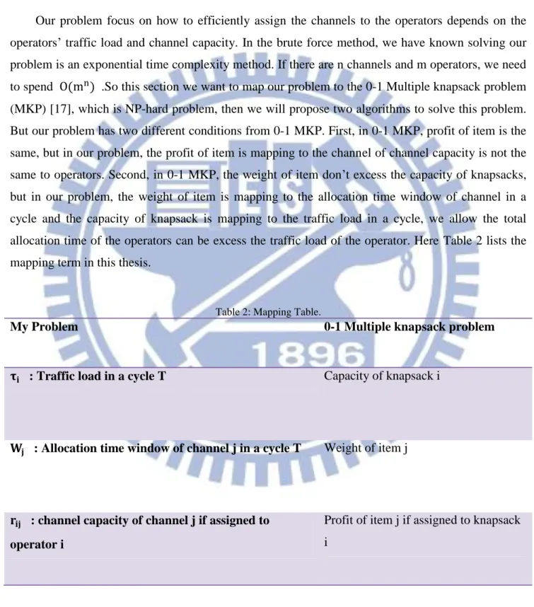
Our problem focus on how to efficiently assign the channels to the operators depends on the operators’ traffic load and channel capacity. In the brute force method, we have known solving our problem is an exponential time complexity method. If there are n channels and m operators, we need to spend .So this section we want to map our problem to the 0-1 Multiple knapsack problem (MKP) [17], which is NP-hard problem, then we will propose two algorithms to solve this problem. But our problem has two different conditions from 0-1 MKP. First, in 0-1 MKP, profit of item is the same, but in our problem, the profit of item is mapping to the channel of channel capacity is not the same to operators. Second, in 0-1 MKP, the weight of item don’t excess the capacity of knapsacks, but in our problem, the weight of item is mapping to the allocation time window of channel in a cycle and the capacity of knapsack is mapping to the traffic load in a cycle, we allow the total allocation time of the operators can be excess the traffic load of the operator. Here Table 2 lists the mapping term in this thesis.

Table 2: Mapping Table.

My Problem 0-1 Multiple knapsack problem

: Traffic load in a cycle T Capacity of knapsack i

: Allocation time window of channel j in a cycle T Weight of item j

: channel capacity of channel j if assigned to

operator i

Profit of item j if assigned to knapsack i

8

3.2 Problem Formulation

In this section, we formulate our problem. Base on the assumptions and system model analysis in last chapter. The problem of our interest is to control the total allocation time of each operator, and find out an optimal channel assignment of operators such that the total channel capacity of primary bands is maximized. The problem is formulated as follows:

∑ ∑ (1) s.t. ∑ { } (2) (3) (∑ ) |∑ | { } (4) where { (5) (6)

Where constraint (2) represents that the channel of primary users can allocate only one operator and all of channels must be allocated to operators. Constraint (4) represent that the total allocation time of each operator compare with its traffic load, if the total allocation time subtracts the operator traffic load is less than zero, then we hope that the less value must be less than the operator traffic load multiply a parameter which is defined in our simulation parameters such that when the output requirement of the assignment result should be guaranteed.

In the following chapter, we will propose two assignment schemes to allocation the channels to operators to meet all the constraint above.

9

Chapter4. The Proposed Methods

In the previous chapter, we map our problem to 0-1 MKP, which is a NP-hard problem. But our problem has two differences with 0-1 MKP as we introduce in last chapter. In [17], we find out a Generalized Assignment problem (GAP) is also similar to our problem, but GAP which is also a NP-hard problem is more complicated than our problem. Hence, our problem can be classified as a NP-hard optimization problem, which cannot be solved in polynomial time. Many algorithms, which can be categorized into two algorithms: exact algorithms and heuristic algorithms, have been proposed to solve the 0-1 MKP and GAP [17]. In this chapter, we describe two optimal solutions with a basic greedy-heuristic algorithm.

4.1 An optimization solution of the objection function

To pursue the optimization solution of this objection function of the problem, we can find all of the possibilities of this problem of all of the constraints. This is a simple way to find the optimization solution of this problem, but it is a very high time complexity method. In this problem, if these are n channels and m operators, the all of the possibilities need to calculate times, so it is not a good solution of this problem. Although, this method is a high time complexity, but it still provides us a simulation result which we compare in the next chapter.

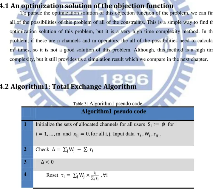
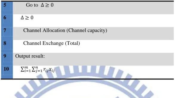
4.2 Algorithm1: Total Exchange Algorithm

Table 3: Algorithm1 pseudo code

_{Algorithm1 pseudo code}

1 Initialize the sets of allocated channels for all users for and . Input data .

2 Check ∑ ∑

3

4 Reset ∑

10

5 Go to

6

7 Channel Allocation (Channel capacity)

8 Channel Exchange (Total)

9 Output result:

10 ∑ ∑

First, we show the first algorithm which is called total exchange algorithm. These are 10 lines of the total exchange algorithm architecture in Table 3. This table focus on solving when the total channel time is less than total traffic load, we handle with the less case into equal case that reduce the traffic load of each operator and reset it by proportion with its origin traffic load of each operator. Then we can focus on channel allocation and exchange part which we show as the following tables.

Table 4: Channel allocation of Algorithm1

Algorithm1 pseudo code

1 { } { } 2 3 4 ( ) 5 6 7

In the Table 4, we allocation the channels to the maximum channel capacity which depends on the each operator. In the following tables, we will show how to use the result of Table 4 to continue channel allocation.

11

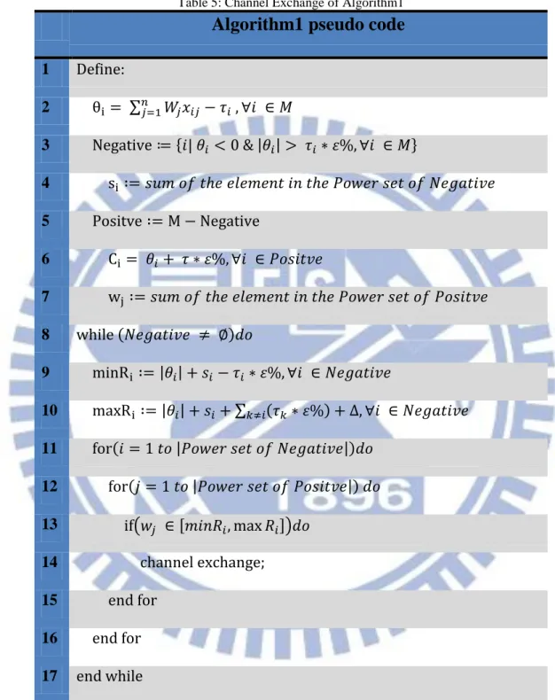
Table 5: Channel Exchange of Algorithm1

Algorithm1 pseudo code

1 2 ∑ 3 { } 4 5 6 7 8 9 10 ∑ 11 12 13 ( [ ]) 14 15 16 17

In Table 5, we show how to channel exchange architecture. In one to seven lines of this table, we divide the operators into two parts; one is positive set which means the allocation time excess than the traffic load of the operator, the other is negative set which means the allocation time excess than

12

the traffic load of the operator. When the negative set is empty, than we finish our allocation algorithm. If the negative set is not empty, than we must do channel exchange which is using the positive set to meet the range that we defined in nine to ten lines, if we find the channels from the positive set than we can exchange the channel to the negative set. In eleven to seventeen lines, we use two for loops to check which channel set can be swap.

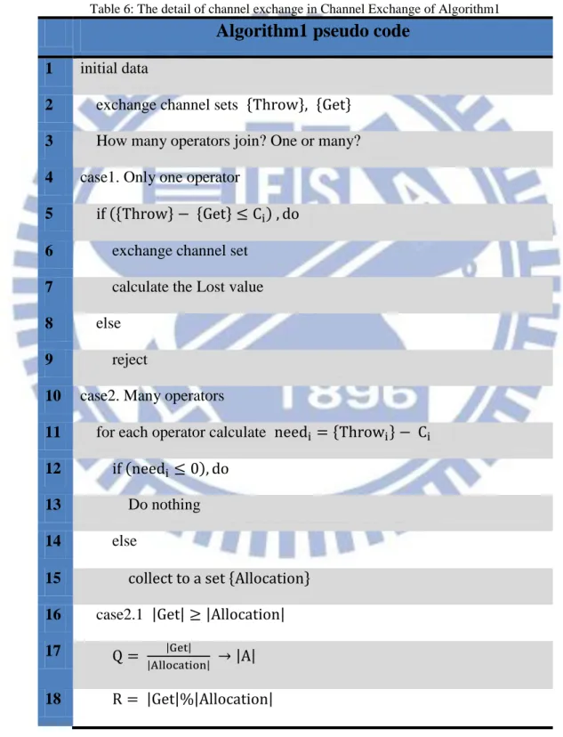
Table 6: The detail of channel exchange in Channel Exchange of Algorithm1

Algorithm1 pseudo code

1 initial data

2 exchange channel sets { } { } 3 How many operators join? One or many?

4 case1. Only one operator

5 { } { }

6 exchange channel set

7 calculate the Lost value

8 else

9 reject

10 case2. Many operators

11 for each operator calculate { }

12 13 Do nothing 14 else 15 { } 16 case2.1 17 18

13 19 case2.1.1 20 case2.1.2 21 case2.1.3 22 case2.1.4 23 case2.1.5 24 calculate the Lost value

25 subcase2.2 26 reject

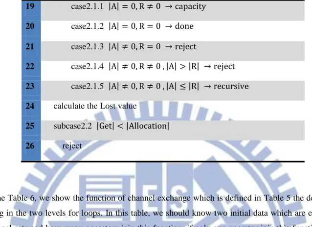
In the Table 6, we show the function of channel exchange which is defined in Table 5 the detail that using in the two levels for loops. In this table, we should know two initial data which are exchange channel sets and how many operators join this function, if only one operator join this function, then we check the sum of the throw set of channels subtracts the sum of the get set of channels whether less than the contribution of the positive operators or not. If the contribution is greater than the subtract result, than we can exchange the channel sets and calculate the lost value. If the above condition isn’t meet it, then we will reject this channel sets. Another condition is many operators joined, we should calculate each operator whether need to be allocated, and then we collect these operators which should be allocated to an allocation set. Next, we should deal with the number of get set greater than or equal the number of allocation set, so when enter this case that we divide into five subcases to handle all of conditions which only one subcase can be finished. In the above tables, we show the detail of total exchange algorithm.

4.3 Algorithm2: Level Exchange Algorithm

Table 7: Algorithm2 pseudo code

_{Algorithm2 pseudo code}

1 Initialize the sets of allocated channels for all users for and . Input data .

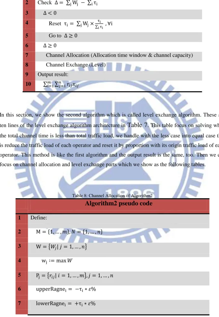
14 2 Check ∑ ∑ 3 4 Reset ∑ ∑ 5 Go to 6

7 Channel Allocation (Allocation time window & channel capacity)

8 Channel Exchange (Level)

9 Output result:

10 ∑ ∑

In this section, we show the second algorithm which is called level exchange algorithm. These are ten lines of the level exchange algorithm architecture in

Table 7

. This table focus on solving when the total channel time is less than total traffic load, we handle with the less case into equal case that is reduce the traffic load of each operator and reset it by proportion with its origin traffic load of each operator. This method is like the first algorithm and the output result is the same, too. Then we can focus on channel allocation and level exchange parts which we show as the following tables.

Table 8: Channel Allocation of Algorithm2

Algorithm2 pseudo code

1 Define: 2 { } { } 3 { } 4 5 { } 6 7

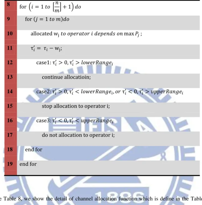
15 8 _{( [ ] )} 9 10 11 12 13 14 15 16 17 18 19

In the Table 8, we show the detail of channel allocation function which is define in the Table 7. In this table, we allocate the channel depends on its maximum capacity of the operators, every operator is allocated one channel in an iteration that is also called a level allocation which means we allocate the channel level by level and in each level, every operator must be allocated unless the last iteration. If this channel assigns the operator which depends on the capacity of this channel, then we check three cases after allocating this channel. When the channel set is empty, the channel allocation function done.

Table 9: Channel Exchange of Algorithm2

Algorithm2 pseudo code

16 2 3 4 5 [ ] 6 7

In the Table 9, we check the situation from the channel allocation function which is defined in the Table 8. When the result of channel allocation is out of the constraint of the problem, then we do channel exchange level by level from the last level to the first level. The channel exchange method is very simple; we interchange the number of operators of the channels of that level. If we finish the channel exchange function, but the channel set isn’t empty, then we allocate the channels of the channel set depends on the capacity of the channels. Its time complexity is much lower than the first algorithm which is an exponential time complexity.

17

Chapter5. Simulation Results

In this chapter, we evaluate the performance of our proposed algorithms and compare with the brute force method. We use C programming language to implement the proposed methods. In this chapter, we will introduce the parameter of simulations and the result of simulations will be shown.

5.1 Parameter setting of simulations

In this section, we will show the parameters of used in our algorithms. This parameter is shown in Table 10.

Table 10: Simulations and analysis parameters

The number of channels 20 The number of operators 3

The constraint of problem 1, 5, 10 The cycle of re-allocation time 1000 second The channel bandwidth 6MHz

The noise power -100 dBm

_{The maximum signal power 50 mW} The arrival rate of PU channel j U(0,1)

The service rate of PU channel j ( ) The number of SU pair of operators [ ]

18

5.2 Simulation Results

We consider three scenarios according to different traffic intensity and different sizes of data. In the three scenarios, we show each parameter of scenario setting in Table 11.

Table 11: Traffic intensity and data size

Scenario1 Scenario2 Scenario3

19

Figure 2: The sum of channel capacity of three methods at different scenarios when

Figure 3: The percentage of two methods compare to brute-force at three scenarios when

In the Figure2 and Figure 3, we combine sum rate of the three scenarios in a graph and show the sum rate of three methods at three scenarios when the constraint is 1. We can see the result of these two figures, the sum rate of the Total-exchange algorithm is very close to the Brute-force method in

4000 4050 4100 4150 4200 4250 4300 4350 4400 4450 1 2 3 Mbps Scenario

The sum of channel capacity

Brute-force Total-exchange Level-exchange 100 100 100 98.3 96.9 98 97.3 95.9 95.1 92 93 94 95 96 97 98 99 100 101 1 2 3

20

the all scenarios, but the sum rate of the Level-exchange algorithm only has the scenario 1 close to the optimal solution. The Level-exchange algorithm depends on the channel capacity of the channels, so the percentage of sum rate of scenario 2 and 3 are lower than the scenario 1.

Figure 4: The sum of channel capacity of three methods at different scenarios when

Figure 5: The percentage of two methods compare to brute-force at three scenarios when 4050 4100 4150 4200 4250 4300 4350 4400 4450 1 2 3 Mbps Scenario

The sum of channel capacity

Brute-force Total-exchange Level-exchange 100 100 100 98.3 98.5 97.2 97.7 96.1 _95.9 93 94 95 96 97 98 99 100 101 1 2 3

21

In the Figure4 and Figure 5, we combine sum rate of the three scenarios in a graph and show the sum rate of three methods at three scenarios when the constraint is 5. We can see the result of these two figures, the sum rate of the Total-exchange algorithm is also very close to the Brute-force method in the all scenarios, comparing with the Figure2 and Figure3. The results of the Level-exchange algorithm are greater than the results of the Figure2 and Figure3. The

Level-exchange algorithm also has the results which is not stable of the sum rate in the scenarios.

Figure 6: The sum of channel capacity of three methods at different scenarios when 4000 4050 4100 4150 4200 4250 4300 4350 4400 4450 1 2 3 Mbps Scenario

The sum of channel capacity

Brute-force Total-exchange Level-exchange

22

Figure 7: The percentage of two methods compare to brute-force at three scenarios when

In the Figure6 and Figure 7, we combine sum rate of the three scenarios in a graph and show the sum rate of three methods at three scenarios when the constraint is 10. We can see the result of these two figures, the results of sum rate of the Total-exchange and the Level-exchange are greater than the Figure4 and Figure5. The Total-exchange algorithm is also very close to the Brute-force method in the all scenarios. The Level-exchange algorithm also has the same condition which is like the Figure4 and Figure5.

100 100 100 99.1 98.7 98.3 97.2 96.7 94.7 92 93 94 95 96 97 98 99 100 101 1 2 3

23

Figure 8: The sum of channel capacity of three methods at different in the Scenario 1

Figure 9: The sum of channel capacity of three methods at different in the Scenario 2 4310 4320 4330 4340 4350 4360 4370 4380 4390 4400 1 5 10 Mbps

scenario1

Brute-force Total-exchange Level-exchange 4260 4270 4280 4290 4300 4310 4320 4330 4340 4350 4360 1 5 10 Mbps

scenario2

Brute-force Total-exchange Level-exchange

24

Figure 10: The sum of channel capacity of three methods at different in the Scenario 3

In the Figure 8, 9, 10 we can see when the from 1 to 10 the sum rate of three methods are ascend, the reason is when the lower range is greater the sum rate will be better, but it’s not fair to the traffic loads of the operators when the from 1 to 10. The total exchange algorithm a very stable algorithm, because it find all of the exchangeable possibilities when the algorithm is executed in the channel exchange step, and it’s an exponential-time algorithm, but its time complexity is still lower than the brute force method. Then, the level exchange algorithm is sufficiently close to the sum rate of the brute force method in the three scenarios. Comparing with the total exchange algorithm, the sum rate of the level exchange algorithm is unstable. Because the level exchange algorithm is sensitive to the channels of channel capacity, but its time complexity isn’t an exponential-time algorithm. It is much faster than the total exchange algorithm, due to when we do channel exchange, the level exchange algorithm will exchange the channels level by level that will reduce the exchange effort.

4200 4220 4240 4260 4280 4300 4320 4340 4360 4380 4400 1 5 10 Mbps

scenario3

Brute-force Total-exchange Level-exchange

25

Chapter6. Conclusion and Future Work

In this thesis, we proposed two channel assignment algorithms to solve our problem and reduce the time complexity of the problem which is an NP-hard problem. One is called total exchange algorithm which is also an exponential-time algorithm - comparing with the brute force method- where m is the number of operators and n denoted the number of channels, the time complexity of total exchange algorithm is less than the brute force method, and the throughput of this algorithm is very close the optimal solution of our problem. The other one is called level exchange algorithm which is not an exponential-time algorithm – ([ ] ) comparing with the brute force method and the total exchange algorithm, the time complexity significantly reduce than the other methods, so this algorithm is much faster than the others, and its throughput is also close the optimal solution of our problem.

In the simulations, we compare throughputs of the algorithm of we proposed, and consider three scenarios. The result of simulations has shown that the throughput of our proposed methods not only reduce the time complexity but also close the optimal solution of our problem.

Our algorithms can also extend to the other problem, such as the product scheduling in the Manufacturing Industry, or resource allocation problems … etc. In the future works, we can improve the throughputs of the algorithm and do the mathematical analysis for the methods.

26

REFERENCES

[1]FCC, ET Docket No 03-222 Notice of Proposed Rule Making and Order,Dec. 2003.

[2]J. Mitola, “Cognitive radio: An integrated agent architecture for software defined radio,” Ph.D. dissertation, KTH Royal Inst. of Technol.,Stockholm, Sweden, 2000.

[3]I. F. Akyildiz, W.-Y. Lee, M. C. Vuran, and S. Mohanty, “Next generation/dynamic spectrum access/cognitive radio wireless networks: A survey,” Comput. Netw., vol. 50, no. 13, pp. 2127–2159, Sep. 2006.

[4] Z. Ji and K. J. R. Liu, “Dynamic spectrum sharing: a game theoretical overview," IEEE Commun.

Mag., vol. 45, no. 5, pp. 88-94, May 2007.

[5] X. Wang, Z. Li, P. Xu, Y. Xu, X. Gao, and H. Chen, “Spectrum Sharing in Cognitive Radio Networks – An Auction-based Approach,” to appear in IEEE Trans. System, Man Cybern, B,

Cybern., 2010.

[6] Y. Hou, Y. Shi, and H. Sherali, “Spectrum sharing for multi-hop networking with cognitive radios,” IEEE Journal on Selected Areas in Communications, vol. 26, no. 1, pp. 146–155, 2008. [7 ]M. Ma and D. Tsang, “Impact of Channel Heterogeneity on Spectrum Sharing in Cognitive Radio Networks,” in IEEE International Conference on Communications, 2008. ICC’08, 2008, pp. 2377–2382.

[8] T. Lv, T. Wang, and X. Yu, “Primary User Activity Based Channel Allocation in Cognitive Radio Networks,” in IEEE Vehicular Technology Conference, 2010, pp. 1–5.

[9] W. Wang and T. Lv, “A Novel Spectrum Sharing Algorithm Based on the Throughput in Cognitive Radio Networks,” IEEE International Conference on Wireless Communications,

Networking and Mobile Computing, Wicom 2009.

[10] Tan and L.T. “Channel Assignment for Throughput Maximization in Cognitive Radio Networks,” in IEEE Wireless Communications and Networking Conference, April 2012, pp. 1427 - 1431

[11] J. Xiang, Y. Zhang, T. Skeie, and J. He, “Qos aware admission and power control for cognitive radio cellular networks,” Wireless Commun. and Mobile Comput., 2009.

[12] A. T. Hoang and Y.-C. Liang, “Downlink channel assignment and power control for cognitive networks,” IEEE Trans. Wireless Commun., vol. 7, no. 8, pp. 3106–3117, Aug. 2008.

[13] M. Ma and Tsang D. H. K., “Impact of channel heterogeneity on spectrum sharing in cognitive radio networks,” Communications, (ICC'08) IEEE Intl. Conf. on, pp. 2377-2382, May 2008.

27

[14] J. Tang, G. Xue, C. Chandler, and W. Zhang, “Link scheduling with power control for throughput enhancement in multihop wireless networks,” IEEE Trans. Veh. Technol., vol. 55, no. 3, pp. 733–742, May 2006.

[15] Y.T. Hou, Y. Shi, and H.D. Sherali. Optimal spectrum sharing for multihop software defined radio networks. Proc. IEEE INFOCOM, May 2007.

[16] S. M. Almalfouh and G. L. Stüber, “Uplink resource allocation in cognitive radio networks with imperfect spectrum sensing,” in Proc. IEEE Veh. Technol. Conf., Sep. 2010, pp. 1–6.

[17] Silvano Martello and Paolo Toth, Knapsack Problems: Algorithms and Computer

Implementations. John Wiley & Sons, 1990.

[18] Donald Gross, John F. Shortle, James M. Thompson, Carl M. Harris, Fundamentals of