建構複合式信用評等模型

全文

(1)國立交通大學工業工程與管理學系碩士論文. 建構複合式信用評等模型 Constructing Hybrid Credit Scoring Model. 研究生：游翔百指導教授：唐麗英. 博士. 中華民國九十三年七月.

(2) 建構複合式信用評等模型 Constructing Hybrid Credit Scoring Model. 研究生：游翔百. Student：Hsiang-Pai Yu. 指導教授：唐麗英博士. Advisor：Lee-Ing Tong. 國立交通大學工業工程與管理學系碩士論文. A Thesis Submitted to Department of Industrial Engineering and Management. College of Management National Chiao Tung University In Partial Fulfillment of the Requirements For the Degree of Master of Science In Industrial Engineering July 2004 Hsin-Chu, Taiwan Republic of China. 中華民國九十三年七月.

(3) 建構複合式信用評等模型. 研究生：游翔百. 指導教授：唐麗英. 國立交通大學工業工程與管理學系碩士班. 摘要風險評估及信用評等是金融機構用以評量借款企業償債能力的重要依據，然而身處目前經濟不景氣的環境下，逐漸身高的逾放比率使得越來越多的金融機構必須檢討其現有信用評等模式的缺失，以對貸款企業做出更正確有效的放款決策。現有之中、外文獻雖發展出許多信用評等模式來探討此問題，一般說來以類神經網路架構出的信用評等模型分類正確率表現較傳統統計方法建構出之模型為佳。但基於類神經網路(Artificial Neural Networks: ANN)理論上的不足，使得類神經網路架構出之信用評等模型解釋能力不佳，在實務層面上難以使用。因而本研究乃針對台灣金融機構之中小企業借款者，發展出一套複合式信用評等模型，此模型流程首先建立分類迴歸樹(Classification and Regression Tree: CART)，然後再將分類迴歸樹的預測結果及事後機率作為後續的類神經網路的輸入變數，藉此來增加整體複合式信用評等模型的分類正確率；此外，藉由使用分類迴歸樹來鑑別具有顯著影響的變數，增加整體複合式信用評等模型的模型解釋能力。同時，本研究也廣泛比較現存的信用評等模型預測能力的差異，分別利用了線性判別分析 (Linear Discriminant Analysis: LDA) 、曲線判別分析 (Quadratic Discriminant Analysis: QDA)、羅吉斯迴歸(Logistic Regression: LR)、機率類神經網路(Probabilistic Neural Network: PNN)、倒傳遞網路(Back Propagation Neural Network: BPN)、一般迴歸神經網路(General Regression Neural Network: GRNN) 、自組性演算法 (Group Method of Data Handling: GMDH)、K 最近鄰居法(K-Nearest Neighbor: KNN)及學習向量量化網路(Learning Vector Quantization Neural Network: LVQ)等不同的信用評等模型，透過台灣某金融機構所提供中小企業借款者的實際歷史資料，驗證了本研究所提出之複合式信用評等模型確實有效可行。【關鍵詞】：信用評等、分類迴歸樹、複合式模型、類神經網路. I.

(4) Constructing Hybrid Credit Scoring Model Student：Hsiang-Pai Yu. Adviser：Lee-lng Tong. Department of Industrial Engineering and Management National Chiao Tung University Abstract Credit scoring is an essential task for banks and loan companies in the last few decades. The demand of developing a credit scoring model with reliable accuracy has become an urgent issue. Among many studies of credit scoring, artificial neural network (ANN) is a promising technique to achieve high accuracy of classification compared to existing conventional techniques. However, the poor explanation power makes ANN difficult to produce interpretable result. This drawback also decreases the power of ANN applied in practical problems. The objective of this study is to propose a hybrid credit scoring model which is combined with CART and other algorithms to enhance the accuracy of credit scoring model, and increase the interpretable capability as well. Financial loan companies can employ this study when establishing their credit scoring models. .. Key Words: Hybrid model, Artificial Neural Network (ANN), Credit Scoring, CART. II.

(5) 誌謝這本論文的完成，有著許多人的幫助與心血。最值得感謝的人是我的指導教授唐麗英博士，若沒有她辛勤的審閱我的論文，這本論文的可讀性一定慘不忍睹。在這兩年的交大研究生活，唐麗英老師啟發了我許多為人處事以及作學問的正確態度，同時也讓我對自己未來的人生規劃，有著更清晰的藍圖。同時，老師對我的諸多提攜，總是提供許多機會讓我去嘗試，像是論文比賽、出國研討會發表論文等，使我在這兩年間大有成長，這都得感謝唐麗英老師。同時感謝口試委員梁高榮教授、王春和教授和計畫書審查委員李慶恩教授提供諸多建議，使得這本論文更臻完善。碩士班兩年非常充實而有趣，感謝實驗室夥伴這兩年的陪伴與協助，千慧學姐、民祥、俊誠、文傑、宏志、冠人、政勳、忠佐、盛全等，我衷心感謝大家，點點滴滴的回憶都將銘記我心。同時，MB606 實驗室的楓凱、淙亮、英泰、士凱等；MB604 實驗室的渙群、石隆；MB002 實驗室的盈月、仁耀；管科所的詠涵、佩雙、慧菁等謝謝你們一路的陪伴，狂歡生日會、螢火蟲夜遊、熬夜寫報告、俊誠家夜烤等等，這些回憶因為有你們的參與，而令人難忘。還得感謝我的女朋友馨平，這兩年她的對我的忍耐與扶持，是我能努力完成此本論文的最大因素，每每碰到挫折與疲累，只有她會一再鼓勵與支持我，讓我持續下去，說她是我精神上的支柱一點也不為過。最後要感謝的是我的父母，這兩年我不常回家，我的父母也毫無怨言，只有辛勤的噓寒問暖，沒有他們，我絕不可能念到碩士學位。僅以此文，向我的父母親及曾幫助我的許多人表達心中最誠摯的感謝。. 游翔百. 謹誌於. 交通大學工業工程與管理研究所 2004 年 7 月 15 日. III.

(6) Contents 中文摘要………………………………………………………….……Ⅰ 英文摘要………………………………………………………….……Ⅱ 誌謝……………………………………………………………….……Ⅲ Contents………………………………………………………….…….Ⅳ List of Figures………………………………………………………....Ⅶ List of Tables…………………………………………………………..Ⅷ Chapter 1 Introduction......................................1 1.1 Background and Motivation...........................1 1.2 Research Objective...................................3 1.3 Organization......................................4 Chapter 2 Literature Review.................................5 2.1 Contemporary credit scoring system of bank loaning.........5 2.1.1 The origin and development of credit scoring.........5 2.2 Discriminant analysis.................................6 2.3 Artificial Neural Networks.............................7 2.4 Other nonparametric methods..........................11 IV.

(7) 2.4.1 Classification and regression tree (CART) ..........11 2.4.1.1 Classification Tree Methodology……..………….11 2.4.1.2 Tree impurity function………………………..13 2.4.1.3 Tree growing methodology…………………..13 2.4.1.4 Tree Pruning…………………...............…………14 2.4.2 Group Methods of Data Handling (GMDH)..............16 2.4.3 General Regression Neural Network (GRNN)............18 Chapter 3 The Proposed Hybrid Model Approach..............20 3.1 Model Evaluation Criterion............................20 3.2 Procedure of Constructing Hybrid Credit Scoring Model....21 3.3 Procedure of Establishing Prediction Model of Default Period.27 Chapter 4 Illustrative Examples.............................31 4.1 Description of Sample Data............................31 4.2 Perform CART.....................................32 4.3 Record CART`s Split Variables and Predictive Outcomes....35 4.4 Use recorded variables and predictive outcomes as input variables of following model.......................35 4.5 Compare The Accuracy of each Hybrid Model and Choose the V.

(8) Best Hybrid Credit Scoring Model......................46 4.6 Establish Prediction Model of Default Period..............46 4.7 Further Comparison of Hybrid Model....................47 Chapter 5 Concluding Remarks .............................50 References..............................................................................52 Appendix..............................................................................55. VI.

(9) List of Figures Figure 1.. Logit tree diagram of credit scoring model................2. Figure 2. The traditional scope of credit scoring model...............3 Figure 3.. Three layer back propagation neural network (BPN).......8. Figure 4.. Example of classification tree..........................12. Figure 5. Geometric Viewpoint of CART...........................13 Figure 6.. Multilayered structure of GMDH with five inputs and selected nodes ...........................................18. Figure 7. Flowchart of the proposed hybrid model....................21 Figure 8.. Hybrid BPN credit scoring model......................27. Figure 9. Flowchart of default period prediction model................29 Figure 10. Original BPN model accuracy...........................38 Figure 11. Hybrid BPN produced by Cart_1.........................39 Figure 12. Hybrid BPN produced by Cart_2.........................39 Figure 13. Hybrid BPN produced by Cart_3.........................40 Figure 14. Hybrid BPN produced by Cart_4.........................40 Figure 15. Hybrid BPN produced by Cart_5.........................41 Figure 16. Hybrid BPN produced by Cart_6.........................41. VII.

(10) List of Tables Table 1. Financial strength ratings of S&P corp. ....................6 Table 2. Merits and demerits of artificial neural networks by Vellido.....10 Table 3. Variable Description....................................31 Table 4. CART candidate models.................................33 Table 5. CART`s split variables...................................33 Table 6. Comparison of original credit scoring models....... .........34 Table 7. Input Variables of following hybrid models.................35 Table 8. Hybrid LDA Performance................................36 Table 9. Original LDA Performance...............................36 Table 10. Hybrid QDA Performance...............................36 Table 11. Original QDA Performance..............................36 Table 12.. Hybrid LR Performance...............................37. Table 13.. Original LR Performance..............................37. Table 14. Hybrid PNN Performance...............................42 Table 15. Original PNN Performance..............................42 Table 16. Hybrid GRNN Performance.............................43 Table 17. Original GRNN Performance............................43 Table 18. Hybrid GMDH Performance.............................43 VIII.

(11) Table 19. Original GMDH Performance............................43 Table 20.. Hybrid KNN Performance.............................44. Table 21.. Original KNN Performance............................44. Table 20.. Hybrid KNN Performance.............................44. Table 21.. Original KNN Performance............................44. Table 22.. Hybrid LVQ Performance.............................45. Table 23. Original LVQ Performance.............................45 Table 24. Best Hybrid Credit Scoring Model......................46 Table 25. The MSE of each prediction model .....................45 Table 26. Variables selected by LDA.............................48 Table 27. The performance of hybrid model based on LDA..........48. IX.

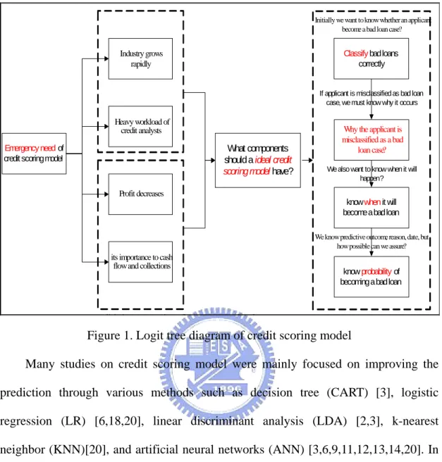
(12) Chapter1 Introduction 1.1 Background and Motivation With rapid growth of the credit industry in last few decades, credit evaluation of loan applicants becomes an important issue not only because the urgent demand from bankers, but also due to the pressure of cash flow and collections [5]. The conventional credit scoring or credit evaluation models simply classify loan applicants into two categories: “Good Loaner” and “Bad Loaner” according to some financial studies. Credit decision-makers can use the result of credit evaluation to make the right judgment and minimize bad loan risk. As a result, credit evaluation received more attention by bankers and a trustworthy credit scoring model became an urgent issue. With a sizable loan portfolio, even slight improvement in the accuracy of credit evaluation can reduce the creditors` risk and translate the accuracy improvement considerably into future savings, cost reduction, faster credit evaluation, and closer monitoring of existing accounts. [5]. In the past, credit scoring was evaluated by creditor analysts. Due to the sharp growth of credit industry, the workload of credit analysts has exceeded its capacity. As a result, finding new automated ways of credit evaluation has become a forthcoming trend. In addition, the risk of potential bad debts is also another critical issue. The depression of financial market made loan applicants of mid-size companies endure greater default pressure than they had in the past. Therefore, loan companies necessitate an accurate credit scoring model urgently to classify loan applicants to alleviate potential loss of bad debt. The percentage of bad loans increases rapidly, credit analysts are looking for strict and objective measures to evaluate loan applicants. All agendas discussed above can be shown in Fig.1. 1.

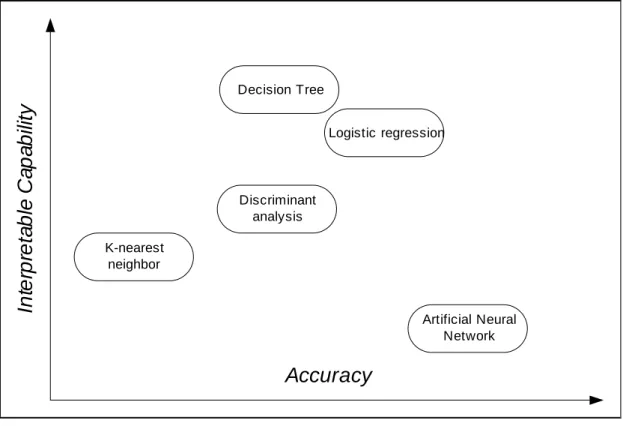
(13) Initially we want to know whether an applicant become a bad loan case?. Classify bad loans correctly. Industry grows rapidly. If applicant is misclassified as bad loan case, we must know why it occurs. Heavy workload of credit analysts. What components should a ideal credit scoring model have?. Emergency need of credit scoring model. Why the applicant is misclassified as a bad loan case? We also want to know when it will happen?. Profit decreases know when it will become a bad loan We know predictive outcome, reason, date, but how possible can we assure?. its importance to cash flow and collections. li h i. i. know probability of becoming a bad loan. di. d. h. Figure 1. Logit tree diagram of credit scoring model Many studies on credit scoring model were mainly focused on improving the prediction through various methods such as decision tree (CART) [3], logistic regression (LR) [6,18,20], linear discriminant analysis (LDA) [2,3], k-nearest neighbor (KNN)[20], and artificial neural networks (ANN) [3,6,9,11,12,13,14,20]. In other words, previous studies elevated on one dimension only--either on classification accuracy or on interpretable capability. Although accuracy or interpretable capability are two major criteria for assessing a credit scoring model, optimizing two major criteria simultaneously are challengeable. That is, pursuing promising classification accuracy and seeking interpretable capability lie on a “trade-off” relation as shown in Fig.2.. 2.

(14) Interpretable Capability. Decision Tree Logistic regression. Discriminant analysis K-nearest neighbor. Artificial Neural Network. Accuracy. Figure 2. Traditional scope of credit scoring model ANN has proved its capability of classification and prediction accuracy in constructing credit scoring model. Many studies indicated that ANN has superior or even dominate accuracy as compared to many conventional statistical classification methods. However, ANN still has some drawbacks such as “black box procedure”, “lack of explanation”, “complex network design”, “lack of feature selection” etc. Among these drawbacks, failing to interpret the classification results is the most controversial problem of ANN. Decision makers occasionally think it is hard to utilize ANN`s results in practice because of the above drawbacks.. 1.2 Research Objective The objectives of this study can be summarized as follows: 1.. Construct a hybrid credit scoring model with superior classification accuracy and interpretable capability than existing credit scoring models.. 2.. Develop a simple feature selection method to enhance the capability of interpretation. 3.

(15) This study utilized decision tree, which adopting classification and regression tree (CART) [4] algorithm, as a feature selection method to choose significant input variables. The chosen variables are then used as inputs for ANN and enhance the total predictive accuracy. In other words, CART can be regarded as a “guide” to construct the credit scoring model, followed by the ANN model to realize not only the influential input variables but also CART`s own classification results. As a result, we may expect the following ANN model or other complex algorithms can learn more accurately and quickly on account of good guide “CART”. Several data mining algorithms were utilized to replace ANN to obtain a best hybrid credit scoring model.. 1.3 Organization The rest of this study is organized as follows. Chapter 2 reviewed the related fundamentals of credit scoring model. Chapter 3 described the proposed method and introduced the model evaluation criterion in detail. Chapter 4 presented the illustrative examples and compared the proposed hybrid approach with existing credit scoring models to demonstrate the effectiveness of the proposed hybrid models. Chapter 5 summarized the result of the study and further research direction.. 4.

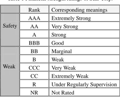
(16) Chapter 2 Literature Review In this chapter, related fundamentals and studies are reviewed. Section 2.1 is a brief introduction of the existing credit scoring system of bank loaning. Section 2.2 discusses reviews the pros and cons of discriminant analysis (DA) used in credit scoring in the past. Section 2.3 presents the artificial neural network (ANN) approach and discusses the related issues of pros and cons. Section 2.4 reviews nonparametric methods and discusses their drawbacks.. 2.1 Contemporary credit scoring system of bank loaning The conventional procedure of constructing a credit scoring of bank loaning is to evaluate the corresponding credit factors such as financial variables and non-financial variables of a company, and credit analysts aggregate the evaluation scores from the credit factors and make the decision. Obviously this procedure lacks objectivity, and credit analysts can easily be misled because of insufficient priori knowledge. Moreover, the result of this credit scoring model may be easily dominated by few key analysts who own the power. Therefore, many studies dedicated to develop a quantitative credit scoring model to avoid shortcomings of the conventional models.. 2.1.1 The origin and development of credit scoring There are over twenty renowned credit scoring companies in the world. “Moody’s”, “Standard & Poor’s (S&P)”, “Fitch IBCA” are three most prominent companies among them and their credit assessing results are widely adopted as external credit scoring models by banks in the whole world. Table 1 presents the rating standard and the corresponding financial strength of companies by S&P. The rating standard can be used as a primary reference for external credit scoring.. 5.

(17) Table 1 Financial strength ratings of S&P corp.. Safety. Weak. Rank AAA AA A BBB BB B CCC CC R NR. Corresponding meanings Extremely Strong Very Strong Strong Good Marginal Weak Very Weak Extremely Weak Under Regularly Supervision Not Rated. 2.2 Discriminant Analysis Linear discriminant analysis (LDA) [17] is the first classification algorithm applied in credit scoring. LDA has been the most commonly used statistical technique in constructing classification model because of its simplicity and popularity. LDA attempts to find a linear combination of predictor variables to classify objects into various groups. Discriminant analysis is designed to maximize the ratio. λ=. γ `Bγ , γ `Wγ. where γ is a p × 1 vector of weights, B and W represent the between-groups and within-group sum of squares for the discriminant function ξ , respectively. The discriminant function is given by. ξ = X `γ , where X is a p × 1 random vector of p variables. Analytically, the objective of DA is to identify the weights γ such that the ratio λ is maximized. Altman [2] collected 33 bankrupt companies and 33 contrary healthy companies to construct a LDA credit scoring model. He found that the linear discriminant credit 6.

(18) scoring model performed very well, especially in short time period. Lee et al. [13] integrated the BPN and LDA approaches to obtain a hybrid credit scoring model and showed that the proposed hybrid approach converges much faster than the conventional BPN model. Moreover, his results indicated that the credit scoring accuracies of the hybrid model outperforms the original BPN, LDA and logistic regression (LR) approaches. A similar study presided by Lee et al. [12] also considered the hybrid neural network models for bankruptcy predictions. Their hybrid methodology contains multiple discriminant analysis (MDA)-assisted neural network, the ID3-assisted neural network operated with the input variables selected by the MDA method and ID3, respectively. They concluded that the hybrid neural network models are very promising for bankruptcy prediction in terms of predictive accuracy and adaptability. Markham and Ragsdale [14] observed that combining the predictions of a well-known statistical tool with one of ANN techniques may provide more accurate prediction results than either individual techniques used alone. They utilized Mahalanobis distance measure (MDM) as inputs of ANN and showed that the hybrid methodology can significantly reduce the average misclassification rate. However, the utilization of LDA in constructing the credit scoring model has received many criticisms because of its theoretical assumptions, such as data must possess a multivariate normal distribution, and the covariance matrices of good loan and bad loan classes must be equal, are frequently violated in real-world data [6,10,20]. Although quadratic discriminant analysis (QDA) can alleviate some drawbacks of LDA, QDA does not perform better than LDA as expected [10,17].. 2.3 Artificial Neural Networks Many researches explored the capability of ANN applied in business problems such as credit scoring or bankruptcy prediction. ANN can learn complex non-linear structure of datasets or can approximate many continuous functions accurately. 7.

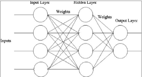
(19) Besides, ANN does not require any priori assumptions about data distribution. A large number of researches and surveys have proven that ANN is a suitable and outstanding technique on extensive business applications [6,9,11,12,13,14,15,18,19,20]. ANN generally consists of three layers: an input layer, a hidden layer, and an output layer. Each layer is interconnected by a number of processing units called “neurons” or “nodes”. Each unit represents a computation device and it transforms an input to an output by means of some pre-specified function. Each link is assigned a numerical value representing the weight of connection. Input nodes receive input signals and aggregate information into hidden layer nodes, and the hidden layer nodes transform the aggregate information into desired targets in output layer nodes by some pre-specified activation function. ANN iteratively adjusts network weights in order to produce desired output as closer as possible. The value of network weight is determined by inputs and outputs of the training dataset through learning algorithms. The objective of ANN is to find a set of appropriate network weights under different network topologies and predict or classify observations accurately. Figure 3 shows a brief presentation of ANN.. Figure 3 Three-layer back propagation neural network (BPN) 8.

(20) Piramuthu et al. [16] used feature construction to improve the performance of ANN and assessed their proposed methodology using Beligian bankruptcy data. Their study concluded that the feature construction improves the searching procedure through the solution-space and increases the average information content of each feature which is used as input to BPN. Olmeda and Fernandez [15] compared the accuracy of several classifiers on the problem of bankruptcy prediction. They concluded that ANN provided the best results compared to logistic regression, DA, C4.5 and multivariate adaptive regression spline (MARs). Tam and Kiang [18] compared a number of well-known classifies such as DA, logistic regression (LR), k nearest neighbor (KNN), ID3, and BPN applied in bank failure predictions. Their results indicated that modified ANN with given prior probabilities and misclassification costs was a promising method of evaluating bank conditions in terms of predictive accuracy, adaptability, and robustness. West [20] investigated the accuracy of credit scoring model constructed using five neural network approaches: multilayer perceptron, mixture-of-experts, radial basis function, learning vector quantization, and fuzzy adaptive resonance. The results are benchmarked against some traditional methods including DA, LR, KNN, kernel density estimation, and CART. His study concluded that BPN may not be the most accurate model and logistic regression is found to be the most accurate traditional method for building a credit scoring model except for ANN approaches. Vellido et al. [19] has surveyed extensively and found that 74 out of 93 papers relied on using the back propagation neural network (BPN), a few others utilized learning vector quantization (LVQ), radial basis function (RBF), self-organization map (SOM), etc. With respect to credit scoring related researches, BPN is the most 9.

(21) widespread model and is often used as a benchmarking approach for other models. Zhang [21] have shown in full details that among all controversial criteria disputed in ANN for classification and summarized, that two of the most important developments in ANN classification were the studies of hybrid neural model and feature selection. One of the disadvantage of ANN is the poor explanatory capability which is referred to as “black box” problem. Because ANN is unable to identify the influential variables or the relevant variables, the result of ANN model may be difficult to achieve rational explanations. Another disadvantage of ANN is that ANN is lack of formal explanation on neural network architecture, that is, there is no formal procedure either to select network topology or to decide network architecture. Vellido [19] indicated that the rule of thumb is the most popular way to select the network topology or decide network architecture. Some researchers such as Glorfeld and Hardgrave [9], Piramuthu et al. [16] endeavored to develop some modification or rules of existing algorithms, but could not obtain satisfactory results. Table 2. Merits and demerits of artificial neural networks by Vellido [19] Merits of artificial neural network y. y. y. y. Demerits of artificial neural network y. Able to learn any complex nonlinear mapping or approximate any continuous function As non-parametric methods, NN do. y. not make any priori assumptions about the distribution of data or input-output mapping function NN are very flexible with respect to incomplete, missing and noisy data, NN are “fault tolerant” Neural network models can be easily updated / are suitable for dynamic environments.. y y. 10. Lack theoretical background concerning explanatory capabilities and results in “black boxes” The selection of the network topology and its parameters lack theoretical background, it is still a “trial and error” matter. Training process of NN is very time-consuming. Neural network can overfit the training data and lose generalization capability..

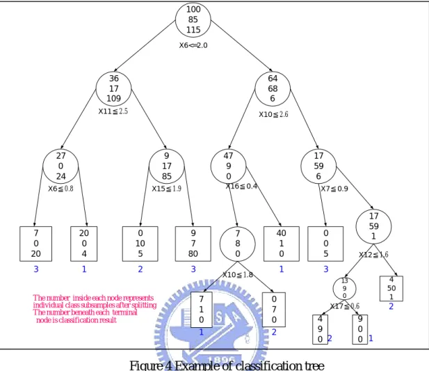
(22) 2.4 Other Nonparametric Methods Nonparametric methods such as LR and CART can be applied in constructing credit scoring model. However, a number of comparative studies indicated that these methods perform well only in specific environment. West [20] also pointed that nonparametric methods do not provide satisfactory outcomes in many studies. However, predictive accuracy is not the only concerned perspective in constructing credit scoring model. Decision tree, K-nearest neighbor (KNN) or other nonparametric methods can also be used as preprocessing mechanisms to enhance the performance of ANN. Vellido [19], Lee et al. [12], Lee et al. [13], Markham and Ragsdale [14] explored the performance of hybrid model and their results showed that the hybrid model performed better than the original ANN methods in respect of predictive accuracy and speed of convergence.. 2.4.1. Classification and Regression Tree (CART). CART [4] is a decision tree method for analyzing categorical data as a function of continuous or categorical explanatory variables. CART uses a set of training samples to grow a classification tree and prune a tree, and finally utilizes a set of testing samples to determine the right size tree which has the lowest misclassification cost.. 2.4.1.1. Classification Tree Methodology. A classification tree T for a categorical variable is constructed by employing recursive partitioning the training samples into two different subsets. The objective is to find the appropriate explanatory variables that can split the training samples as correct as possible according to some pre-specific splitting criteria. The subsamples are called leaf nodes or nodes. The entire original training samples are noted as root node t1 of the tree. Similarly, the descendent nodes are abbreviated as tL for the left subsamples. Subsamples which are not split further are called the terminal nodes. Graphically, the nodes and splitting rules denoted under each node are depicted in 11.

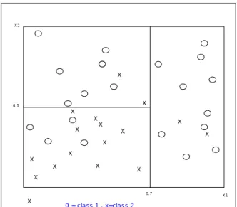
(23) Fig.4. 100 85 115 X6<=2.0. y y. 36 17 109. 64 68 6. X11≦2.5. X10≦2.6. 27 0 24. 9 17 85. X6≦0.8. X15≦1.9. 47 9 0 X16≦0.4. 7 0 20. 20 0 4. 0 10 5. 9 7 80. 3. 1. 2. 3. The number inside each node represents individual class subsamples after splitting The number beneath each terminal node is classification result. 17 59 6 X7≦0.9. 7 8 0 X10≦1.8. 7 1 0 1. 40 1 0. 0 0 5. 1. 3. 0 7 0 2. 17 59 1 X12≦1.6 4 50 1. 13 9 0. X17≦0.6. 4 9 0 2. 2. 9 0 0 1. Figure 4 Example of classification tree The splitting criterion of CART is to split the training sample into two subsamples. Each of the subsamples contains only cases from one category. In this case, the split decreases the most impurity of parent node, in other words, the tree can be thought of as a “partitioning hyperplane into rectangle” such that the populations within each rectangle become more and more homogeneous. Fig.5 depicts the case. The impurity measure i(t) of node t is defined as i(t)=ψ(p(1|t),p(2|t)…,p(J| t)). The node impurity is the largest when all classes are equally mixed together in node, and it becomes the smallest n the case where the node contains only one class. Our goal is to decide the best split which decreases the impurity as much as possible.. ∆i ( s, t ) = i (t ) − pLi(tL ) − pRi(tR ). 12.

(24) X2. X. X. 0.5. X X. X. X. X. X. X. X X X X. X. X. X 0.7. X. X1. 0 = cla ss 1 , x=cla ss 2. Figure 5 Geometric Viewpoint of CART. 2.4.1.2. Tree impurity function. A tree impurity I(T) can be defined as follows:. I (T ) = ∑ I (t ) =∑ i(t ) p(t ) ~ t∈T. ~ t∈T. Maximizing the decrease in tree impurity I(T) by splitting the number “s＂ on node t is given as follows:. ∆I ( s, t ) = I (t ) − I (tL ) − I (tR ) = ∆i ( s, t ) p(t ). 2.4.1.3. Tree growing methodology. There are five steps for employing tree growing methodology: 1.. Decide impurity function. 2.. Grow tree by maximizing tree impurity decrease until the tree size become as large as possible.. 3.. Get the best tree by pruning structure.. 4.. Use the proper “estimation method＂ to get estimator of classifier.. 5.. Interpretation results.. 13. tree.

(25) 2.4.1.4. Tree pruning. In CART algorithm, it adopts “Minimal cost-complexity pruning” to prune the tree: ~ Rα (T ) = R (T ) + α T. Rα (T (α )) = min Rα (T ) T ≤Tmax. Above formula implies that α can be thought as the complexity cost per terminal node and Rα is an linear combination of the total misclassification error R(T) ~ and its complexity cost α T of subtree T. As the penalty costαof complexity per. terminal node increases, the minimizing subtrees T(α) will have fewer terminal nodes. When α is large enough, the subtree T(α) will eventually consist of the root only, and the tree Tmax will be completely pruned. The pruning outcomes are expected to be:. Tmax > T1 > T2 > ..... > {t1} However, the above outcomes are hard to achieve. Neither T1>T2, nor T2 is necessarily pruned from previous subtree T1. Direct search through all possible subtrees to find Rα(T) is computationally expensive. As a result, Breiman [3] used “Weakest-Link. cutting”. for. any. non-terminal. node. t. of. Tmax. which. appears R(t ) > R(Tt ) . Actually t can be thought as the survival node of pruned tree after removing branch tree Tt.. Rα ({t}) = R(t ) + α × 1 ~ ~ R α (T t ) = R (T t ) + α × T t 14.

(26) The subtree t means the subtree contains only one terminal node t, and its misclassification error is R(T), and its penalty cost of complexity is α × 1 ; Similarly, The subtree Tt. means the subtree contains. ~ Tt. terminal nodes, and its. ~ misclassification error is R(Tt), and its penalty cost of complexity is α × Tt .. In many cases, the misclassification error R(t) is bigger than R(Tt), the fact can be explained that the subtree Tt has more complex structure and then have better classification capability compared to subtree t . It also means that subtree Tt has better classification capability than subtree t. However, if Rα (Tt ) = Rα ({t}) , the {t} subtree is preferable because subtree t. and subtree Tt have the same sum of misclassification error and penalty cost of complexity. That is, although the subtree Tt has smaller misclassification error R(T) ~ than subtree t, after considering the penalty cost of complexity α × Tt , both of the. two subtrees perform equivalently. According to the parsimonious rule, the subtree t is preferable. In order to find the critical value α, the following inequality is solved: R α (Tt ) < R α ({t}) ⇒α<. R(t ) − T (Tt ) ~ T t. Define function g1(t), where t belongs to T1, as:. ~ ⎧ R(t ) − R(Tt ) ⎪ T~ − 1 , t ∉ T1 g1 (t ) = ⎨ t ~ ⎪ ⎩+ ∞, t ∈ T1 15.

(27) Define weakest link t1 in T1 as:. g1 (t1 ) = min g1 (t ) t∈T1. α 2 = g1 (t1 ) The node t1 is the weakest link when the parameter α increases, t1 is also the first node such that Rα({t}) become equal to Rα(Tt), and then the simple subtree{ t1 } is preferable to the complex subtree Tt , and α2 is the value of α at which equality occurs. Finally, a list of pruned T(αk) trees can be obtained when α increases. The best pruned classification tree will be constructed.. 2.4.2 Group Methods of Data Handling (GMDH) Group Method of Data Handling (GMDH) [1] is applied in a great variety of areas in data mining. Inductive GMDH algorithms aim to find interrelations of variables in a data set and select the optimal structure of a model or a network. GMDH is an iterative method which successively tests models selected from a set of candidate models according to a specified criterion. General connection between input and output variables can be found in the form of a functional Volterra series, whose discrete analogue is known as the Kolmogorov-Gabor polynomial. The polynomial can be expressed as follows, M. M. M. i =1. i =1 j =1. M. M. M. y = a 0 + ∑ a i x i + ∑∑ a ij x i x j + ∑∑∑ a ij x i x j x k + ... i =1 j =1 k =1. where X = ( x1 , x 2 , x 3 ,..., x M ) is the vector of input variables and. 16.

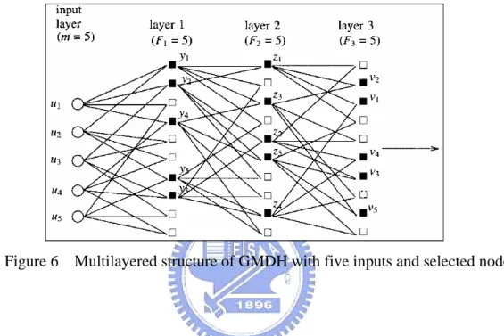
(28) A = (a1 , a 2 , a 3 ..., a M ) is the vector of summand coefficients. The combinational GMDH algorithm has a multilayer iterative structure. Its specific feature is that the iteration rule does not remain consistent but expands with each new series. In the first series, all the models of the simplest structure are in the following form. y = a 0 + ai xi. i = 1,2,..., M. After sorting these models, select the best F models by specified criterion. Models are sorted by series of equal structure complexity and best model is found for each series according to the specified criterion. In the second series, models of more complex structure are sorted. These models are constructed on output variables from the best models of the first series:. y = a 0 + ai xi + a 2 x j. i = 1,2,..., F ; j = 1,2,..., M . F ≤ M .. In the third series, the sorting involves more complex structure of the form as follows:. y = a0 + ai xi + a 2 x j + a3 x k i = 1,2,..., F ; j = 1,2,..., F . k = 1,2,..., M F ≤ M .. The iterative procedure of the series continues until the criterion value stop increasing. More complex iterative multilayered GMDH algorithm can be obtained by similar ways. The iteration rule remains the same for all series. For example, the form. y = a 0 + a1 x i + a 2 x j + a 3 x j x i is used in the first series, and a particular description. z = b0 + b1 y i + b2 y j + b3 y j y i in the second series, and a particular description. 17.

(29) w = c 0 + c1 z i + c 2 z j + c 3 z j z i is used in the third series, and so on. That is, the output values of a previous series are served as augments in the next series. The final model can be decided by specified external and internal criterion. The multilayered structure of GMDH algorithm can be shown in Fig.6.. Figure 6 Multilayered structure of GMDH with five inputs and selected nodes. 2.4.3 General Regression Neural Network (GRNN) General regression neural network (GRNN) [7] is a one-pass learning network with a highly parallel structure. The algorithm can be used for any regression problems in which linearity assumption is not justified. GRNN provides estimates of continuous variables and converges to the underlying regression surface. Suppose that f ( x, y ) represents the known joint continuous probability density function. The regression of y on X is given by ∞. E[y | X ] =. ∫ yf ( X , y )dy. −∞ ∞. .. ∫ f ( X , y )dy. −∞. When the density f ( x, y ) is unknown, it must be estimated from observations 18.

(30) of x and y. GRNN utilizes kernel density regression approach which adopted Parzen windows estimation fˆ ( X , Y ) =. 1 ( 2π) ( p +1) / 2 σ ( p +1). ⎡ (Y − Y i ) 2 ⎤ ⎡ ( X − X i )T ( X − X i ) ⎤ 1 n exp exp ∑ ⎢− ⎥ ⎢− ⎥ n i =1 2σ 2 2σ 2 ⎦ ⎣ ⎦ ⎣. to estimate f ( x, y ) . By using Parzen windows estmation, the GRNN estimator can be easily presented as the following equation: ⎡ ( X − X i )T ( X − X i ) ⎤ ∞ ⎡ ( y − Y i )2 ⎤ y − exp exp ∑ ⎢ ⎥∫ ⎢− ⎥dy 2 2 σ σ 2 2 i =1 ⎣ ⎦−∞ ⎣ ⎦ Yˆ ( X ) = ∞ i T i i 2 n ⎡ (y −Y ) ⎤ ⎡ (X − X ) (X − X )⎤ exp ⎢ − ∑ ⎥dy ⎥ ∫ exp ⎢ − 2 2σ 2 ⎦ 2σ i =1 ⎣ ⎦−∞ ⎣ n. Di2 is defined as the a scalar function as follows: Di2 = ( X − X i ) T ( X − X i ) Performing the substitution of Di2 yields the following GRNN estimator: ⎡ Di2 ⎤ i exp ⎢ − ∑ ⎥Y 2σ 2 ⎦ i =1 ⎣ Yˆ ( X ) = . n ⎡ Di2 ⎤ exp ⎢ − ∑ 2 ⎥ i =1 ⎣ 2σ ⎦ n. 19.

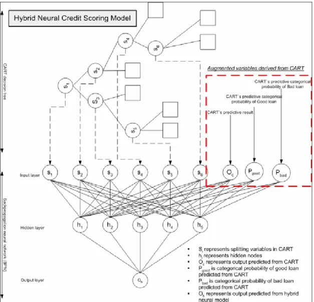
(31) Chapter 3 The Proposed Hybrid Model Approach As mentioned in chapter 2, the feature selection problem is the main shortcoming in employing ANN to construct a neural network based credit scoring model. The hybrid model approach received a lot of attentions recently. Most of the studies on hybrid models are constructed by combining statistical method and ANN. The analytical procedure of credit scoring model proposed by this study mainly consists of two phases. In the first phase, the hybrid credit scoring model is composed of Classification and regression trees (CART) and other data mining algorithms such as BPN, LVQ, LDA etc. The first phase employs CART`s predictive outcome and predictive categorical probability as input variables to construct the subsequent models using BPN, LDA, etc. The purpose of the first phase is to present a hybrid credit scoring model with higher accuracy and greater interpretable capability than the original credit scoring models without using hybrid approach. In the second phase, a predictive model of default period will be built through various data mining algorithms to obtain a precise estimator of default period. That is, for bad loaners, the time period between the loan start and the loan default is defined as the “default period”. The objective of the second phase is to present a effective model to predict the default period of default-possible cases.. 3.1 Model evaluation criterion Financial loan companies often encounter considerable default loss due to misjudging or misclassifying the bad loan cases into “good loan” category. On the contrary, the loan companies will lose potential revenues if a good loan applicant is misclassified into “bad loan” category. The misclassified bad loan cases cause much greater loss to financial loan companies than misclassified good loan cases. Thus the prediction accuracy of “bad loan” is the higher the better for loan companies to 20.

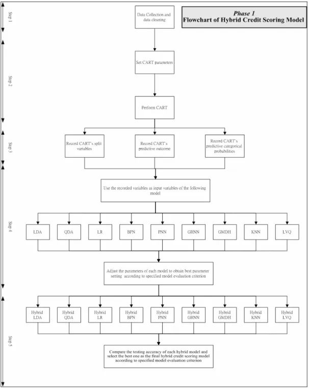
(32) maintain an acceptable default risk. In this study, the good loan accuracy is specified to be greater than 50% to retain the essential profit.. 3.2 Procedure of Constructing Hybrid Credit Scoring Model Phase 1：Construct Proposed Hybrid Credit Scoring Model. The proposed procedure of phase 1 can be shown in Fig. 7. Each step in phase1 is described as follows:. Figure 7. Flowchart of the proposed hybrid model 21.

(33) Step1: Data collection and cleaning. Loan applicants in this study are mid-sized companies whose financial statements are not as credible as those of public offering companies. Therefore, financial statement is only one part of considerable factors in this study. Loan companies usually adopt financial variables (quantitative factor) and non-financial variables (qualitative factor) simultaneously to increase model accuracy and reliability. This study collected loan data from a loan company in Taiwan in 2000 to 2003 as sample data and divided the dataset into two categories: “bad loan” and “good loan”. If a loan applicant is classified into “bad loan” category, the loan will be default and become a bad debt according to the proposed credit scoring model. On the contrary, “good loan” means the loan applicant can reimburse its debt in time. Step2: Perform CART. The procedure of constructing CART can be described as follows: Step 1. Decide impurity function. Step 2. Grow tree by maximizing the decrease of tree impurity until the tree size becomes as large as possible. Step 3. Prune tree structure. Step 4. Use proper estimation method to obtain the honest estimator of tree classifier. The default setting is 10-fold cross validation. Step 5. Interpret the results. Step3: Record CART`s split variables and predictive outcomes. In Step3, split variables of CART models can be deemed as the influential variables and should be recorded for further Steps. Similarly, CART`s predictive. 22.

(34) outcome and CART`s predictive categorical probabilities can be deemed as important compressed information derived from CART model and should be retained as well. As a result, even the number of input variables of the hybrid model decreases, the model accuracy can still be retained using CART`s predictive outcomes and CART`s predictive categorical probabilities as input variables. Step4: Use recorded variables and predictive outcomes as input variables of following model. CART has selected significant variables in Step3, therefore most of the relevant information are retained in the following three variables: “CART`s predictive categorical probability of bad loan”, “CART`s predictive categorical probability of good loan” and “CART`s predictive outcome”. These variables can be used as augmented input variables of the subsequent model to enhance the accuracy of the hybrid model. Fig. 8 displays an example of CART`s recorded variables which can be used as input variables of following BPN model. Similarly, these three recoreded variables can be introduced to other algorithms such as LDA, LR, etc. This study also adopted many data mining algorithms to replace BPN to examine the effectiveness of proposed hybrid model. The cases given below described the credit scoring models constructed using the algorithm specified in each case. Case 1. Linear Discriminant Analysis (LDA): Specify appropriate prior probabilities for each category and utilize LDA to obtain results. LDA is performed using SAS 8.1 and the classification result is evaluated through N-fold cross validation. Case 2. Quadratic Discriminant Analysis (QDA): Specify appropriate prior probabilities for each category and utilize QDA to obtain results. QDA is performed using SAS 8.1 and the classification. 23.

(35) result is evaluated through N-fold cross validation. Case 3. Logistic Regression (LR): Specify appropriate probability threshold value and utilize LR to obtain results. LR is performed using SAS 8.1 and the classification result is evaluated through hold-out method. 80% of data are chosen randomly to construct the LR model and the rest 20% of data are taken to validate the accuracy of LR model. Case 4. Back Propagation Neural network (BPN): The architecture of BPN [10] is decided to be three-layer BPN with completely interconnected neurons. With regard to the number of hidden nodes, this study adopted cascade learning rule to decide the proper number of hidden nodes. That is, cascade learning rule implies that hidden nodes increase gradually until the prediction accuracy of “testing bad loan” is not increased. As regards to the learning rate, momentum, and learning epochs, this study decided to use a small learning speed and long learning epochs to avoid the disturbance of overfitting. However, testing accuracy is another critical perspective when setting the number of epochs. The detail setting of network parameters are adhere to above principles. BPN is performed using Neural Shell2 (NeuralWare) and the classification result is evaluated through hold-out method. 80% of data are chosen randomly to train the BPN model and the rest 20% of data are used to validate the accuracy of BPN model. Case 5. Probabilistic Neural network (PNN): The architecture of PNN [10] can be easily determined from the observations of dataset. The only parameter which necessitates to be manually set is the smoothing parameter. This study adopts cascade 24.

(36) learning to decide best smoothing parameter. PNN is performed using Neural Shell2 (NeuralWare) and the classification result is evaluated through hold-out method. 80% of data are chosen randomly to train the PNN model and the rest 20% of data are used to validate the accuracy of PNN model. Case 6. General Regression Neural network (GRNN): The architecture of GRNN can also be easily determined from the observations of dataset as the same as PNN. The only parameter which necessitates manually setting is the smoothing parameter. This study here also adopts cascade learning to decide best smoothing parameter. GRNN is performed using Neural Shell2 (NeuralWare) and the classification result is evaluated through hold-out method. 80% of data are chosen randomly to train the GRNN model and the rest 20% of data are used to validate the accuracy of GRNN model. Case 7. Group Method of Data Handling (GMDH): GMDH is performed using Neural Shell2 (NeuralWare) and the classification result is evaluated through hold-out method. 80% of data are chosen randomly to train the GMDH model and the rest 20% of data are used to validate the accuracy of GMDH model. Case 8. K-Nearest Neighbor (KNN): It needs to set two parameters in training KNN [10], the first is the number of “K”, which represents the number of nearest neighbors, and the other is the measure of distance. This study utilizes Euclidean distance as measure of distance while performing KNN. As for the number “K”, rule of thumb (trial and error) method is employed to decide the best value for K. KNN is performed using Matlab6.5 25.

(37) (MathWorks inc) and the classification result is evaluated through hold-out method. 80% of data are chosen randomly to train the KNN model and the rest 20% of data are used to validate the accuracy of KNN model. Case 9. Learning Vector Quantization (LVQ): It needs to set three parameters mainly in training LVQ [10]. The first parameter is the number of prototypes, and another is learning rate and the other is the measure of distance. As for the number of initial prototypes, rule of thumb (trial and error) method is employed to decide the best value for the number of prototypes. Besides, the initial prototypes can be determined through random selection from the training samples. With respect to learning rate, preliminary experiments indicated the learning rate has no significant impacts for LVQ results. Hence this study set the value 0.1 as the learning rate. Similarly, this study utilizes Euclidean distance as measure of distance while performing LVQ. With respect to learning epochs, the number of learning epochs is not the critical factor in training LVQ because LVQ converges very fast. Thus the value of learning epochs is set to be 15. LVQ is performed using Matlab6.5 (MathWorks) and the classification result is evaluated through hold-out method. 80% of data are chosen randomly to train the LVQ model and the rest 20% of data are used to validate the accuracy of LVQ model.. 26.

(38) Figure 8. Hybrid BPN credit scoring model Step5: Compare the accuracy of hybrid credit scoring model and select the best one as the final model.. The final credit scoring model is selected from the nine cases described in Step4. In other words, nine hybrid credit scoring models are constructed in Step4. According to the model evaluation criterion, select the best one as the final hybrid credit scoring model from the nine hybrid credit scoring models.. 27.

(39) 3.3 Establish Prediction Model of Default Period Phase 2：Establish Prediction Model of Default Period. For bad loaners, the time period between the loan start and the loan default is defined as the “default period”. Default period means the time period in which loaner still reimburse his debt regularly, the longer default period means the less potential profit loss to loan companies. On the contrary, the shorter default period represents the greater default risk. This phenomenon often makes loan companies unable to take proper reactions in time to the loan applicants with short default period. Therefore, loan companies can take precautions and adopt corresponding reactions to the possible-default cases by reexamining the predicted default period when the loan applicant is classified into “Bad loaner category” in phase 1. Fig.9 describes the proposed procedure of phase 2.. 28.

(40) Figure.9 Flowchart of default period prediction model Each step in phase2 is described as follows: Step 1: Data collection and cleaning. The term “Default period” is only defined for bad loaners. The phase 2 simply choose bad loan data as sample data. Therefore, a prediction model of default period can be established through the bad loan cases. In addition, casewise deletion is adopted in this step. Step 2: Model construction. This study employs three data mining algorithms to predict default period and the result of the three models are compared with the linear regression model. Three data mining algorithms are given below. Case 1.Back Propagation Neural network (BPN): The setting of parameters and network architecture are determined as mentioned in phase 1. Case 2.General Regression Neural network (GRNN): The setting of parameters and the GRNN network architecture are determined as mentioned in phase 1. Case 3.Group Method of Data Handling (GMDH): The setting of parameters and GMDH architecture are determined as mentioned in phase 1. Step 3: Model comparison. The criterion for model comparison is mean square error (MSE). MSE is the smaller the better. The small MSE represents small difference between predicted output and the target. As a result, select the model with minimum value of testing MSE as the final model of default period. The MSE of linear regression is treated as a 29.

(41) benchmarking method in this step.. 30.

(42) Chapter 4 Illustrative Examples 4.1 Description of Sample Data The illustrative examples in this study consisted of 2080 commercial bank loaners, of which 1709 good loan cases and 371 bad loan cases. These data were obtained from a famous financial loan company in Taiwan for the period 2000 to 2003. Each loan case included 31 variables of interest and some of these variables are non-financial variables. The variables are predetermined by the financial loan company. Detail descriptions of variables in the study are summarized in Table 3. It is noticeable that there are 14 financial variables and 17 non-financial variables, in which financial variables were directly measured from the financial statements and non-financial. variables. were. indirectly. measured. by. analysts`. subjective. determination. From the practical point of view, both financial and non-financial variables were used to construct the credit scoring model in this study. Table 3. Variable Description Rating Items. Variable Code. Rating Items. K83. Own capital rate. N1. History. K85. Debit ratio. N2. Employee`s Loyalty. K87. Fix ratio. N3a. Background. K93. Current ratio. N3b. Capability. K95. Rapid ratio. N4. Company Wealth. K97. DSR. N5. Credibility of Financial statement. K100. Turnover days of Net value. N11. Legal Policy. Variable Code. Financial structure (N6). Liquidity Capability (N7) Management Capability. 31.

(43) K102. Turnover days of account receivable. N12. Economic Factor. K104. Inventory Turnover. N13. Industry Trend. K107. Gross profit rate. N14. Production capability. K109. Net profit rate. N15. Marketing & Sales capability. K111. EPS. N16. Management Teams capability. K114. Growth rate of EPS. N17. Evaluation by competitors and customers. K116. Growth rate of sales volume. Net_Value. Net Value. Default Period. Default Period. SCORE. Subtotal scores. Capital. Capital of company. (N8). Profitability (N9). Growth Power (N10). 4.2 Perform CART This study used CART 5.0 sponsored by Salford systems to perform CART. After setting the minimum complexity α equal to zero and favor even split equal to 1, many preliminary experiments indicated that appropriate CART models can be obtained by adjusting prior probabilities shown in table 2. Besides, this study repeats the proposed procedure of phase 1 six times to generate six different CART candidate models, and then use the six CART candidate models to construct the hybrid models. This practice intended to verify the effectiveness of the hybrid models produced by different CART candidate models. In. 32.

(44) other words, if the hybrid model performs well under whichever the CART candidate models is selected, the hybrid model approach can be deemed as an effective methodology. Table 4 and displays the six different CART candidate models. The detail model of six CART candidate models can be found in Appendix. Table 4. CART candidate models. Impurity function. Number of split variables. Candidate1. GINI. Candidate2. CART model. Testing Accuracy Abbreviation of the model. Good loan. Bad loan. 12. 57.109. 71.429. Cart_1. GINI. 14. 54.535. 72.507. Cart_2. Candidate3. GINI. 11. 50.673. 73.315. Cart_3. Candidate4. GINI. 10. 51.668. 73.046. Cart_4. Candidate5. GINI. 15. 55.12. 72.237. Cart_5. Candidate6. GINI. 9. 51.551. 73.315. Cart_6. The split variables of each produced CART model are listed in table 5. Significant reduction of input variables can be observed in table 5. Furthermore, these split variables can be regarded as influential variables and be used to construct the hybrid model. Table 5. CART`s split variables CART model. Number of split variables. Split variables. Candidate1. 12. N4 N5 N6 N7 N14 K95 K97 K104 K107 K109 Capital Net_Value. Candidate2. 14. Candidate3. 11. N3 N4 N5 N6 N7 N9 N14 N15 K104 K107 K109 K116 Capital Net_Value N4 N6 N9 N14 N15 N17 K85 K97 K109 Capital Net_Value. 33.

(45) Candidate4. 10. N4 N6 N9 N14 N15 K85 K97 K109 Capital Net_Value. Candidate5. 15. N3 N4 N6 N7 N9 N14 N15 K87 K95 K97 K104 K107 K109 K116 Net_Value. Candidate6. 9. N4 N6 N7 N14 N15 N17 K85 K97 Net_Value. Apparently, the original CART does not provide satisfactory results under anyone of the six candidate models. Other original credit scoring models were also established and summarized in Table 6 as benchmarking methods. This study adopted an extensive trial and error method to find the best parameter setting for each model. After many preliminary experiments, the best parameter setting and testing accuracy of each original model can be obtained and showed in Table 6. Table 6. Comparison of original credit scoring models Testing Accuracy (%) Model. Abbreviation. Notes Bad Loan. Good Loan. Linear Discriminant Analysis. LDA. 79.51. 50.46. Priors: 0.63 :0.37. Quadratic Discriminant Analysis. QDA. 76.01. 51.61. Priors: 0.66 :0.34. Logistic Regression. LR. 79.2. 51. Probability level: 0.12. Classification & Regression Tree. CART. 73.04. 51.66. Priors: 0.59 :0.41. Probabilistic Neural Network. PNN. 52.05. 77.26. Smoothing factor 0.355. Backpropagation Neural Network. BPN. 82.19. 51.31. Hidden node: 15. General Regression Neural Network. GRNN. 81.03. 62.56. Smoothing factor 0.6583. Group Method of Data Handling. GMDH. 82.27. 50.74. Criterion value 0.150836. K-Nearest Neighbor. KNN. 25.28. 86.93. K=1. 34.

(46) Learning Vector Quantization. LVQ. 29.88. 93.27. Prototypes: 400. 4.3 Record CART`s Split Variables and Predictive Outcomes Spilt variables, predictive categorical probabilities and predictive result of CART were recorded and used as input variables for the further hybrid models.. 4.4 Use recorded variables and predictive outcomes as input variables of following model The three variables: spilt variables, predictive categorical probabilities and predictive result were used as input variables in LDA, QDA, BPN, etc. The input variables of the following hybrid model are summarized in Table 7. Table 7. Input Variables of following hybrid models Input variables of following hybrid models CART model Split variables Candidate1. N4 N5 N6 N7 N14 K95 K97 K104 K107 K109 Capital Net_Value. Candidate2. N3 N4 N5 N6 N7 N9 N14 N15 K104 K107 K109 K116 Capital Net_Value. Candidate3. N4 N6 N9 N14 N15 N17 K85 K97 K109 Capital Net_Value. Candidate4. N4 N6 N9 N14 N15 K85 K97 K109 Capital Net_Value. Candidate5. N3 N4 N6 N7 N9 N14 N15 K87 K95 K97 K104 K107 K109 K116 Net_Value. Candidate6. N4 N6 N7 N14 N15 N17 K85 K97 Net_Value. Augmented variables from CART model. Predictive probability of bad loan of CART.. Predictive probability of good loan of CART.. Predictive outcome of CART.. The procedure of constructing various hybrid models followed the principles described in Step 4 in section 3.2. This study used SAS 8.1 to perform LDA, QDA. 35.

(47) and LR analysis. According to each CART candidate model, a corresponding hybrid model was built and shown as table 8. Case 1. Linear Discriminant Analysis (LDA):. The performance of hybrid LDA model and the original LDA model was compared and the results were listed in Table 8 and Table 9. Obviously, the accuracy of hybrid LDA model for the testing bad loan was significantly higher than the original LDA by 5% no matter which CART candidate model was used. Table 8. Hybrid LDA Performance. Table 9. Original LDA Performance. Hybrid LDA. Original LDA N-fold CV. Hybrid LDA model. Bad:Good. Cart_1. Prior. N-fold CV. accuracy(%). Priors. LDA model. Bad:Good. Bad loan. Good loan. 0.69:0.31. 83.02. 50.2. LDA-1. Cart_2. 0.61:0.39. 88.14. 54.18. Cart_3. 0.70:0.3. 85.41. Cart_4. 0.66:0.34. Cart_5 Cart_6. accuracy(%) Bad loan. Good loan. 0.60:0.40. 77.9. 55.12. LDA-2. 0.61:0.39. 78.44. 53.66. 51.96. LDA-3. 0.62:0.38. 78.71. 52.31. 84.59. 50.19. LDA-4. 0.63:0.37. 79.51. 50.46. 0.64:0.36. 82.43. 51.96. LDA-5. 0.64:0.36. 80.32. 48.57. 0.66:0.34. 82.7. 51.08. The best five LDA models. Case 2. Quadratic Discriminant Analysis (QDA):. Table 10 and Table 11 also indicated that the hybrid QDA had better prediction accuracy than the original QDA model. Obviously, the testing bad loan accuracy of hybrid QDA model increased at least by 7% compared to the original QDA no matter which CART candidate model was used. Table 10. Hybrid QDA Performance. Table 11. Original QDA Performance. Hybrid QDA. Original QDA 36.

(48) N-fold CV Hybrid QDA model. Prior Bad:Good. N-fold CV QDA Model. accuracy(%) Bad loan. Good loan. Priors Bad:Good. accuracy(%) Bad loan. Good loan. Cart_1. 0.73:0.27. 83.02. 59.74. QDA-1. 0.62:0.38. 73.85. 57.99. Cart_2. 0.74:0.26. 83.29. 59.57. QDA-2. 0.63:0.37. 74.66. 56.52. Cart_3. 0.50:0.5. 82.16. 49.39. QDA-3. 0.64:0.36. 75.2. 55. Cart_4. 0.52:0.48. 82.16. 50.85. QDA-4. 0.65:0.35. 75.74. 53.13. Cart_5. 0.50:0.5. 82.97. 45.64. QDA-5. 0.66:0.34. 76.01. 51.61. Cart_6. 0.56:0.44. 84.05. 50.53. The best five QDA models. Case 3. Logistic Regression (LR):. Similar results as in Case 1 and Case 2 can be observed in Table 12 and Table 13. This also indicated that the hybrid LR model significantly performed better than the original LR model according to the specified model evaluation criterion. Table 12. Hybrid LR Performance. Table 13. Original LR Performance. Hybrid LR Hybrid LR model. Probability level. Cart_1. Original LR Testing accuracy(%). LR model. Probability level. Bad loan. Good loan. 0.12. 84.1. 50. LR-1. Cart_2. 0.08. 87.1. 57.6. Cart_3. 0.10. 83.2. Cart_4. 0.12. Cart_5 Cart_6. Testing accuracy(%) Bad loan. Good loan. 0.12. 79.2. 51. LR-2. 0.14. 75.5. 57.8. 57.6. LR-3. 0.16. 72.2. 65.2. 83.2. 55.4. LR-4. 0.18. 68.2. 70.9. 0.12. 81.4. 55.5. LR-5. 0.20. 65.2. 75.6. 0.08. 88.1. 51. The best five LR models 37.

(49) Case 4. Back Propagation Neural network (BPN):. The procedure of BPN can be stated as follows: a very small learning rate at 0.001, momentum as 0.85, and learning epoch as 2000 are set in the BPN training period to avoid overfitting problem and fluctuation of predictive accuracy. With regard to the number of hidden nodes, this study adopted cascade learning rule to decide the proper number of hidden nodes. Cascade learning rule implies that hidden nodes increase gradually until the accuracy of testing bad loan stop increasing. For instance, the results of cascade learning procedure were plotted in Fig.10 and Fig.11. Moreover, Fig.10 and Fig.11 also indicated that the prediction accuracy of hybrid BPN model produced by Cart_1 increased up to 10% as compared to the original BPN model. Other hybrid BPN models also have the same improvement on the bad loan accuracy.. Bad loan accuracy is around 75%~80%. Good loan accuracy is around 50%~55%. Fig.10. Original BPN model accuracy. 38.

(50) Bad loan accuracy is around 87%~90%. Good loan accuracy is around 55%~60%. Fig.11. Hybrid BPN produced by Cart_1. Bad loan accuracy is around 87%~90%. Good loan accuracy is around 55%~60%. Fig.12. Hybrid BPN produced by Cart_2. 39.

(51) Bad loan accuracy is around 85%~90%. Good loan accuracy is around 55%~58%. Fig.13. Hybrid BPN produced by Cart_3. Bad loan accuracy is around 87%~90%. Good loan accuracy is around 50%~55%. Fig.14. Hybrid BPN produced by Cart_4. 40.

(52) Bad loan accuracy is around 90%~95%. Good loan accuracy is around 55%~60%. Fig.15. Hybrid BPN produced by Cart_5. Bad loan accuracy is around 85%~90%. Good loan accuracy is around 50%~55%. Fig.16. Hybrid BPN produced by Cart_6 Obviously, Fig.11-Fig.16 indicated the significant effectiveness by using hybrid model approach. The prediction accuracy of bad loan increases at least by 10%~15%.. 41.

(53) The accuracy of good loan also increases by 5%. The performance of the proposed hybrid BPN exceeds what we expected according to specified model evaluation criterion. Case 5. Probabilistic Neural network (PNN):. Even Probabilistic Neural network (PNN) is adopted, the same improvement of prediction accuracy can be obtained in Table 14 and Table 15. The results in these tables also indicated that hybrid PNN model performed significantly better than the original PNN model. Table 14. Hybrid PNN Performance. Table 15. Original PNN Performance. Hybrid PNN Hybrid PNN model. Smoothing factor. Cart_1. Original PNN Testing accuracy(%). PNN model. Smoothing factor. Bad loan. Good loan. 0.1808. 71.23. 81.87. PNN-1. Cart_2. 0.1730. 63.01. 90.53. Cart_3. 0.1500. 56.06. Cart_4. 0.2545. Cart_5 Cart_6. Testing accuracy(%) Bad loan. Good loan. 0.2375. 33.33. 85.88. PNN-2. 0.2515. 42.86. 80.92. 76.44. PNN-3. 0.2375. 34.38. 82.62. 72.97. 86.26. PNN-4. 0.2375. 31.67. 84.46. 0.1691. 64.86. 84.41. PNN-5. 0.3550. 52.05. 77.26. 0.2118. 63.51. 89.71. The best five PNN models. Case 6. General Regression Neural network (GRNN):. As compared to the original credit scoring models, GRNN performed best among all original models. The performance of hybrid GRNN model is still quite good. Almost 5% to 10% accuracy improvement was obtained when hybrid GRNN model was employed. Table 16 and Table 17 indicated that hybrid GRNN model performed significantly better than the original models. 42.

(54) Table 16. Hybrid GRNN Performance. Table 17. Original GRNN Performance. Hybrid GRNN Hybrid GRNN model. Smoothing factor. Cart_1. 0.2972. Cart_2. Original GRNN. Testing accuracy(%). Testing accuracy(%). GRNN model. Smoothing factor. 87.83 56.72. GRNN-1. 0.6777. 81.03 57.82. 0.4370. 93.24 57.89. GRNN-2. 0.6661. 79.31 62.01. Cart_3. 0.3205. 90.54 56.14. GRNN-3. 0.6816. 81.03 59.77. Cart_4. 0.4836. 86.48 63.15. GRNN-4. 0.6816. 81.03 60.33. Cart_5. 0.3128. 82.18 61.26. GRNN-5. 0.6505. 81.03 62.29. Cart_6. 0.3943. 81.08 64.91. Bad loan. Good Loan. Bad loan. Good loan. The best five GRNN models. Case 7. Group Method of Data Handling (GMDH):. GMDH did not perform well as compared to the original models. However, hybrid GMDH model had surprisingly promising accuracy in all GMDH hybrid model. Almost 10% accuracy improvement was obtained when hybrid GMDH was e,ployed. Table 18 and Table 19 indicated that the hybrid GMDH model performed significantly better than original models.. Table 18. Hybrid GMDH performance. Table 19. Original GMDH performance. Hybrid GMDH. Original GMDH. Hybrid GMDH model. Cart_1. Testing accuracy(%) Bad loan. Good loan. 87.83. 50.87. GMDH model. GMDH-1. 43. Testing accuracy(%) Bad loan. Good loan. 74.13. 49.72.

(55) Cart_2. 91.89. 56.43. GMDH-2. 82.27. 50.74. Cart_3. 87.83. 57.01. GMDH-3. 80.95. 51.27. Cart_4. 90.54. 53.50. GMDH-4. 77.77. 50.99. Cart_5. 89.18. 55.26. GMDH-5. 73.01. 52.12. Cart_6. 90.54. 51.46. The best five GMDH models. Case 8. K-Nearest Neighbor (KNN):. KNN did not result in satisfactory result. The prediction accuracy of bad loan for KNN models is far lower than 50% which is requested by the model evaluation criterion. Although the total accuracy of both good loan and bad loan is still quite promising, the fact that KNN can`t incorporate different objectives of various categories make KNN hard to be applied in constructing the credit scoring model. Similarly, the performance of hybrid KNN models also produced disappointed results. Theoretically, the possible reason for the poor classification capability of KNN might be inferred to the extremely gap of sample sizes between bad loan class and good loan class. Prototype methods such as KNN classify observation according to the major class of “K” nearest neighbors. That is, if the difference of sample size between bad loan class and good loan class become extremely big, the “K” nearest neighbors might all belong to the same category. However the phenomenon is not induced by the general KNN classification rule but induced by the extremely difference of sample size between bad loan class and good loan class. Table 20. Hybrid KNN Performance. Table 21. Original KNN Performance. Hybrid KNN Hybrid KNN model. Neighbor number K. Original KNN Testing accuracy(%) Bad loan. KNN model. Good loan. 44. Neighbor number K. Testing accuracy(%) Bad loan. Good loan.

(56) Cart_1. 1. 36.48 86.55. KNN-1. 1. 25.28. 86.93. Cart_2. 1. 22.89 86.48. KNN-2. 2. 25.28. 86.93. Cart_3. 1. 30.45 86.45. KNN-3. 3. 17.24. 96.04. Cart_4. 1. 32.14 87.04. KNN-4. 4. 17.24. 95.75. Cart_5. 1. 29.11 87.53. KNN-5. 5. 14.94. 97.87. Cart_6. 1. 33.33 88.06. The best five KNN models. Case 9. Learning Vector Quantization (LVQ):. The performance of LVQ is as poor as that of KNN. The reason might be the same as for the poor performance of KNN. Both LVQ and KNN are prototype methods theoretically, as a result, the similar depressed result of LVQ is likely to be anticipated. Table 22 and Table 23 showed the performance of hybrid LVQ and original LVQ models. However, 10% to 15% improvement in prediction accuracy for bad loan can be still observed in Table 22. Table 22. Hybrid LVQ Performance. Table 23. Original LVQ Performance. Hybrid LVQ Hybrid LVQ model. Prototype number K. Original LVQ Testing accuracy(%) Bad. Good. loan. loan. LVQ model. Prototype number K. Testing accuracy(%) Bad. Good. loan. loan. Cart_1. 250. 27.02 94.44. LVQ-1. 100. 26.43. 92.40. Cart_2. 150. 31.08 93.86. LVQ-2. 250. 27.58. 91.18. Cart_3. 200. 37.87. LVQ-3. 300. 22.98. 92.09. Cart_4. 200. 33.33 88.82. LVQ-4. 350. 22.98. 91.18. Cart_5. 250. 27.84 87.24. LVQ-5. 400. 29.88. 92.70. 92. 45.

(57) Cart_6. 300. 23.45 91.94. The best five LVQ models. 4.5 Compare the accuracy of each hybrid model and choose the best hybrid credit scoring model The final hybrid credit scoring model can be easily derived from the Table 24. Table 24. Best Hybrid Credit Scoring Model Hybrid Model. Method. Bad loan Accuracy. Good loan Accuracy. Note. Rank. 1st. Cart_2+GRNN. CART + GRNN. 93.24. 57.89. Smoothing factor: 0.4370. Cart_2+ BPN. CART + BPN. 93.24. 57.01. Hidden nodes: 5. 2nd. Cart_2+ GMDH. CART + GMDH. 91.89. 56.43. Criterion Value: 0.1396. 3rd. The Hybrid model “Cart_2+GRNN” is the final hybrid credit scoring model with the highest prediction accuracy. Nearly 15% improvement in prediction accuracy of bad loan was obtained when the original best model was compared with this hybrid model. The result of proposed hybrid model demonstrated the fact that no matter which the CART candidate model is selected, or whatever the following algorithms is utilized, the prediction accuracy of the proposed hybrid model is always significantly higher than original models. The result also strongly support that CART can be used as the feature selection method to enhance the classification accuracy.. 4.6 Establish Prediction Model of Default Period The term “Default period” is only defined for bad loaners. This study chose bad 46.

(58) loan data as the sample data to construct the prediction model of default period. Therefore, the prediction model of default period can be established through the bad loan cases in phase 2. In addition, casewise deletion is adopted here. The testing MSE of each prediction model of default period is summarized in Table 25. The prediction model with the minimum testing MSE was selected as the final prediction model of default period. The procedure and principles of constructing each prediction model were the same as described in the previous Sections. The stepwise linear regression model is also constructed as a benchmarking method and the comparisons of various prediction models of default period are shown in Table 25. Table 25. The MSE of each prediction model Prediction Model. MSE. Rank. GMDH. 20.354. 1st. BPN. 21.927. 2nd. GRNN. 23.468. 3rd. Linear Regression. 32.678. 4th. According to Table 25, GMDH is chosen to be the final prediction model of default period. Hence, the default period can predict more precisely by GMDH than any other models.. 4.6 Further Comparison of Hybrid Model We are now in a position to say the fact that using CART as a preprocessing mechanism or feature selection tool can definitely increase the model accuracy. The results derived from many algorithms have verified the generalization capability of the proposed hybrid CART model. The concept of proposed model can be easily applied in other classification methods such as Support Vector Machine (SVM) [10, 11]. However, it is still a doubtful point: Can we use other algorithms rather than. 47.

(59) CART? Shall the performance of other classification tools (Such as LDA) perform better than the proposed hybrid model built from CART? As the question noted earlier, the study explored the hybrid model which adopted LDA as feature selection method in phase1.The similar procedure mentioned in chapter 3 is utilized to construct the hybrid model derived from LDA. First, the variables selected by LDA, the LDA`s predicted outcome and LDA`s predicted categorical probabilities were adopted as input variables of the following models. These chosen variables of LDA are listed in Table 26. Table 26. Variables selected by LDA Input Variables of following hybrid models. LDA Model. Augmented Variables from LDA. Discriminator Variables. Posterior probability of bad loan of LDA.. LDA. N1 N2 N4 N5 N7 N13 N14 N15 K85 K87 K97 K109 Net_Value. Posterior probability of good loan of LDA.. Predictive outcome of LDA.. In addition, Table 27 indicated the result of LDA based hybrid model has inferior accuracy than CART based hybrid model no matter what the subsequent model was used. 5% to 10% degradation of accuracy can be observed in Table 27. Table 27. The performance of hybrid model based on LDA Hybrid Model. Bad loan Accuracy. Good loan Accuracy. Compare to Original Model. Compare to Hybrid model based on CART. LDA+BPN. 84.93. 53.06. Better. Worse. 48.

(60) LDA+GRNN. 83.56. 50.72. Better. Worse. LDA+GMDH. 81.08. 52.92. Better. Worse. Consider the illustrative example given above, the hybrid model based on CART does have better performance than LDA based models. Although the prediction accuracy of hybrid model based on LDA increases slightly more than the original models, this study still recommend to use the proposed model to obtain accurate prediction results.. 49.