多台攝影機之靜態與動態校正技術

全文

(1)國立交通大學電子工程學系電子研究所. 博士論文多台攝影機之靜態與動態校正技術. Static and Dynamic Calibration of Multiple Cameras. 研. 究. 生：陳宜賢. 指導教授：王聖智. 博士. 中華民國九十七年一月.

(2)

(3) 多台攝影機之靜態與動態校正技術. Static and Dynamic Calibration of Multiple Cameras. 研究生：陳宜賢. Student: I-Hsien Chen. 指導教授：王聖智博士. Advisor: Dr. Sheng-Jyh Wang. 國立交通大學電子工程學系電子研究所博士班博士論文 A Dissertation Submitted to Department of Electronics Engineering & Institute of Electronics College of Electrical Engineering and Computer Science National Chiao Tung University in Partial Fulfillment of the Requirements for the Degree of Doctor of Philosophy in Electronics Engineering January 2008 Hsinchu, Taiwan, Republic of China. 中. 華. 民. 國. 九. 十. 七年. 一. 月.

(4)

(5) 多台攝影機之靜態與動態校正技術. 研究生：陳宜賢. 指導教授：王聖智博士. 國立交通大學電子工程學系電子研究所. 博士班. 摘要在本論文中，我們提出兩個新穎且有效的攝影機校正技術。第一個是多台攝影機的靜態校正方法，其以同一平面上的簡單物體之影像，投影回空間為基礎;另一個則是多台攝影機的動態校正技術，其以單一攝影機所拍之畫面在時間軸上的變化，以及多台攝影機之間的相對方位為基礎。我們所採用的系統模型，能普遍適用於大部分配有多台攝影機的監控系統，不論是靜態或動態校正方法，都不需要特別的系統架設或使用特定的校正樣本。值得一提的是，我們的動態校正技術不用作複雜的特徵點對應技術。此論文所提的多台攝影機之靜態校正，是指尋找攝影機之間的相對位置和方向。一開始我們先推導在攝影機傾斜角度的變化下，三度空間和攝影機影像的座標轉換關係，此對應關係建立之後，再透過攝影機觀察水平面上的簡單物體，來估測此攝影機的擺放高度及其傾斜角度。接著，依據每台攝影機所估測的傾斜角度和高度，我們將各攝影機所觀測到的同一向量，投影回三度空間中，藉著比較此向量的空間座標，各攝影機之間的相對方位即可很容易地被估測出來。就某個方面來看，我們的方法可被視為將 homography 矩陣的運算，拆解成兩個簡單的校正過程，因此可以減少多台攝影機校正的運算量。除此之外，不需要使用到座. i.

(6) 標化的校正樣本，而我們的校正結果可以提供較直接的幾何感覺。本論文亦討論關於參數波動和測量誤差的敏感性分析，我們將數學分析的結果和電腦模擬的結果都呈現出來以驗證我們的分析，實際影像的實驗結果也展現此方法的功效和可行性。至於動態校正的問題，我們推測多台攝影機的左右轉動角度（pan angle）和傾斜角度（tilt angle）的變化情況。在這個部分中，我們將左右轉動角度的因素考慮進來，並且重新建立在攝影機左右轉動、以及上下轉動的情況下，三維空間中水平面和二維影像的對應關係，以此關係為基礎，利用影像特徵點的位移情形，和多台攝影機之間所形成的 epipolar 平面的約束，來估測各台攝影機左右轉動角度和傾斜角度的變化。此方法不需要複雜的特徵點對應技術，而且也允許移動物體出現在校正場景中，這樣的動態校正過程，對於主動式之視訊監控的相關應用將會非常地有用。此外，我們也從數學上去探討了關於測量誤差和前次估測誤差的敏感性分析，從模擬的結果，證明了左右轉動角度和傾斜角度的變化之估計誤差，在實例中是可被接受的。而此方法的功效和可行性也在實際場景的實驗中展現出來。. ii.

(7) Static and Dynamic Calibration of Multiple Cameras. Student：I-Hsien Chen. Advisor：Dr. Sheng-Jyh Wang. Department of Electronics Engineering & Institute of Electronics National Chiao Tung University. Abstract In this dissertation, we present two new and efficient camera calibration techniques. The first one is the static calibration for multiple cameras, which is based on the back-projections of simple objects lying on the same plane. The other one is the dynamic calibration for multiple cameras, which is based on the temporal information on a single camera and the relative space information among multiple cameras. We adopt a system model that is general enough to fit for a large class of surveillance systems with multiple cameras. Both our static and dynamic calibration methods do not require particular system setup or specific calibration patterns. It is worthwhile to mention that, for our dynamic calibration, no complicated correspondence of feature points is needed. Hence, our calibration methods can be well applied to a wide-range surveillance system with multiple cameras. In the problem of static calibration for multiple cameras, we infer the relative positioning and orientation among multiple cameras. The 3D-to-2D coordinate transformation in terms of the tilt angle of a camera is deduced first. After having established the 3D-to-2D transformation, the tilt angle and altitude of each camera are iii.

(8) estimated based on the observation of some simple objects lying on a horizontal plane. With the estimated tilt angles and altitudes, the relative orientations among multiple cameras can be easily obtained by comparing the back-projected world coordinates of some common vectors in the 3-D space. In some sense, our approach can be thought to have decomposed the computation of homography matrix into two simple calibration processes so that the computational load becomes lighter for the calibration of multiple cameras. Additionally, no coordinated calibration pattern is needed and our calibration results can offer direct geometric sense. In this dissertation, we also discuss the sensitivity analysis with respect to parameter fluctuations and measurement errors. Both mathematical analysis and computer simulation results are shown to verify our analysis. Experiment results over real images have demonstrated the efficiency and feasibility of this approach. In the problem of dynamic calibration, we infer the changes of pan and tilt angles for multiple cameras. In this part of the thesis, we take the pan angle factor into account and re-build the mapping between a horizontal plane in the 3-D space and the 2-D image plane on a panned and tilted camera. Based on this mapping, we utilize the displacement of feature points and the epipolar-plane constraint among multiple cameras to estimate the pan-angle and tilt-angle changes for each camera. This algorithm does not require a complicated correspondence of feature points. It also allows the presence of moving objects in the captured scenes while performing dynamic calibration. This kind of dynamic calibration process can be very useful for applications related to active video surveillance. Besides, the sensitivity analysis of our dynamic calibration algorithm with respect to measurement errors and fluctuations in previous estimations is also discussed mathematically. From the simulation results, the estimation errors of pan and tilt angle changes are proved to be acceptable in real cases. The efficiency and feasibility of this approach has been iv.

(9) demonstrated in some experiments over real scenery.. v.

(10) vi.

(11) 誌. 謝. 有幸得王聖智教授的殷切指導，使我的人生有了一條很不一樣的路。在漫長的研究過程中，非常感謝王老師很費心思地跟我討論問題、督促我，訓練我獨立研究的精神，在辯證問題的過程中，有時候還得容忍我說話的任性，真的很感謝他，我才能在艱辛的學位求取過程走到最後。在此，我要將這份得之不易的榮耀，獻給我最摯愛的家人，特別感謝我的父親、母親，在我遇到挫折時，適時地提供鼓勵與支持，並堅定我的信念，也謝謝妹妹宜妙，由於曾經是實驗室的一員，更能體會研究和攻讀博士所承受的壓力，因此常成為我傾吐宣洩苦悶的對象。還有謝謝正民的陪伴，在這同樣的人生階段，我們一起互相勉勵。另外，感謝實驗室學長陳信嘉、陳俊宇適時的鼓勵和開導，還有學弟們在求學上、生活上的相互支持，同時為我的研究生活增添色彩。也要謝謝師母的關心和照顧，讓我在研究之餘，能注意健康和保養身體。一路走來，很幸運地有大家的關心和扶持，真的很謝謝你們。最後，對於口試委員們陳稔博士、黃仲陵博士、宋開泰博士、張隆紋博士、洪一平博士、陳永昇博士、陳祝嵩博士以及王老師，感謝你們的建議和指導，尤其是陳永昇老師，曾經不吝於提供我研究上的解惑，在此致上最誠摯的敬意。. 陳宜賢. vii. 2008 年 1 月.

(12) viii.

(13) Contents ______________________________________________. 摘要 ................................................................................................................................i Abstract ........................................................................................................................ iii 誌謝 .............................................................................................................................vii Contents ........................................................................................................................ix List of Tables.............................................................................................................. xiii List of Figures .............................................................................................................xiv List of Notations ...................................................................................................... xviii Introduction..................................................................................................................1 1.1. Dissertation Overview ........................................................................................1. 1.2. Organization and Contribution .........................................................................5. Backgrounds .................................................................................................................7 2.1. Projective Geometry ...........................................................................................7. 2.1.1 Perspective Projection ........................................................................................8 2.1.2 Epipolar Geometry ...........................................................................................10 2.1.3 Homography......................................................................................................12 2.2. Camera Calibration ..........................................................................................15 ix.

(14) 2.2.1 Calibration with Three-Dimensional Objects ................................................15 2.2.2 Calibration with Planar Objects......................................................................16 2.2.3 Calibration with One-Dimensional Objects ...................................................19 2.2.4 Self-Calibration .................................................................................................21 2.3. Dynamic Camera Calibration..........................................................................24. Static Calibration of Multiple Cameras...................................................................27 3.1. Introduction of Our Camera Model Syatem ..................................................28. 3.1.1 System Overview...............................................................................................28 3.1.2 Camera Setup Model ........................................................................................29 3.2. Pose Estimation of a Single Camera................................................................31. 3.2.1 Coordinate Mapping on a Tilted Camera.......................................................31 3.2.2 Constrained Coordinate Mapping...................................................................32 3.2.3 Pose Estimation Based on the Back-Projections ............................................32 3.2.3.1 Back-Projected Angle w.r.t. Guessed Tilt Angle..........................................34 3.2.3.2 Back-Projected Length w.r.t. Guessed Tilt Angle .......................................37 3.3. Calibration of Multiple Static Cameras..........................................................40. 3.3.1 Static Calibration Method of Multiple Cameras ...........................................40 3.3.2 Discussion of Pan Angle....................................................................................42 3.4. Sensitivity Analysis............................................................................................44. 3.4.1 Mathematical Analysis of Sensitivity ..............................................................47 3.4.2 Sensitivity Analysis via Computer Simulations..............................................47 3.4.2.1 Sensitivity w.r.t. u0 and v0 ..............................................................................49 3.4.2.2 Sensitivity w.r.t. α and β.................................................................................49 3.4.2.3 Sensitivity w.r.t. ∆xi’ and ∆yi’ ........................................................................49 3.4.2.4 Sensitivity w.r.t. Different Choices of Tilt Angle .........................................50 3.5. Experiments over Real Images ........................................................................55 x.

(15) 3.5.1 Calibration Results ...........................................................................................55 3.5.2 Discussion and Comparison with the Homography Technique....................60 Dynamic Calibration of Multiple Cameras .............................................................65 4.1. Dynamic Calibration of Multiple Cameras ....................................................66. 4.1.1 Coordinate Mapping on a Tilted and Panned Camera .................................67 4.1.2 Dynamic Calibration of a Single Camera Based on Temporal Information ... .............................................................................................................................68 4.1.3 Dynamic Calibration of Multiple Camera Based on Epipolar-Plane Constraint ...................................................................................................................70 4.2. Dynamic Calibration with Presence of Moving Objects ...............................77. 4.3. Sensitivity Analysis............................................................................................86. 4.4. Experiments over Real Scenes .........................................................................91. Conclusions.................................................................................................................99 Bibliography ..............................................................................................................103 Curriculum Vita..........................................................................................................107. xi.

(16) xii.

(17) List of Tables ______________________________________________. Table 3.1: Variations of Tilt Angle and Altitude with respect to Different Parameter Fluctuations and Measurement Errors...............................................49 Table3.2: Variations of Tilt Angle and Altitude with respect to Different Choices of Tilt Angle...........................................................................................53 Table 3.3: Upper Table: Estimation of Tilt Angle and Altitude. Lower Table: Spatial Relationship among Cameras.............................................................56 Table 3.4: Mean Absolute Distance and Standard Deviation of the Point-wise Correspondence.............................................................................62 Table 4.1: Variations of Estimation Results with respect to Previous Estimation Errors and Measurement Errors......................................................................88 Table 4.2: Variations of Estimation Results with respect to Distance Fluctuations in Epipolar Lines..................................................................................88 Table 4.3: Results of the Static Calibration...............................................................92. xiii.

(18) List of Figures ______________________________________________. Fig. 1.1. An example of images captured by a camera mounted on the ceiling…....3. Fig. 1.2. An image pair with two different views. Green lines indicate three pairs of corresponding epipolar lines................................................................4. Fig. 2.1. Pinhole imaging model [3, p. 4].....................................................................9. Fig. 2.2. Perspective projection coordinate system [3, p. 28].…………………........9. Fig. 2.3. Illustration of epipolar-plane constraint……...............................................11. Fig. 2.4. A homography between two views [44, p. 325]..........................................12. Fig. 2.5. A homography compatible with the epipolar geometry [44, pp. 328].........13. Fig. 2.6. The fundamental matrix can be represented by F = [e]× H Π , where H Π is the projective transform from the second to the first camera, and [e]× represents the fundamental matrix of the translation [44, p. 250].....14. Fig. 2.7. A 3-D calibration pattern with regularly arranged rectangles……...........16. Fig. 2.8. Camera imaging system of a one-dimensional object [12]……..................20. Fig. 2.9. An example of the calibration operation by using a 1-D object with a fixed point [12].................................................................................20. Fig. 2.10 The epipolar tangency to the absolute conic images [18]……..................22 Fig. 3.1 Flowchart of the proposed static calibration procedure.............................28. xiv.

(19) Fig. 3.2. Model of camera setup................................................................................29. Fig. 3.3. Geometry of a horizontal plane ∏ with respect to a tilted camera….........31. Fig. 3.4. (a) Rectangular corner captured by a tilted camera (b) Illustration of back-projection onto a horizontal plane on for different choices of tilt angles…………….…………………………………………………......35. Fig. 3.5. Back-projected angle with respect to guessed tilt angles........................36. Fig. 3.6 Back-projected length with respect to guessed tilt angle. Each curve is generated by placing a line segment on some place of a horizontal plane...................................................................................................38 Fig. 3.7. (a) Top view of two cameras and a vector in the space (b) The world coordinates of the vector with respect to these two cameras….........40. Fig. 3.8. (a) Three points marked in the image captured by a PTZ camera (b) Top view of the back-projected corners and the optical axes with respect to different guessed pan angles…………………………..…................42. Fig. 3.9. (a) Top view of line segments placed on a horizontal plane (b) Top view of corners placed on a horizontal plane…………………………...................47. Fig. 3.10 Variations of the (a) L-v.s.-φ curves and (b) ψ-v.s.-φ curves with respect to the variation of v0...............................................................................50 Fig. 3.11 Variations of the (a) L-v.s.-φ curves and (b) ψ-v.s.-φ curves with respect to the variation of β..................................................................................51 Fig. 3.12 Sensitivity w.r.t. fluctuations of xi’ and yi’..................................................52 Fig. 3.13 (a) Test image (b) Deduced ψ-v.s.-φ curves (c) Deduced L-v.s.-φ curves....55 Fig. 3.14 (a) Test image captured by four cameras (b) Top view of the relative positions between four cameras................................................................58 Fig. 3.15 Evaluation of calibration results……….…………………………………59 Fig. 3.16 Test images with a rectangular calibration pattern………………………60 Fig. 3.17 Evaluation of calibration results by using five points. (a) Point correspondence based on the homography technique. (b) Point correspondence based on the proposed method……..............................62 Fig. 4.1 Flowchart of the proposed dynamic calibration algorithm......................65 xv.

(20) Fig. 4.2. Illustration of a pseudo plane Π’..................................................69. Fig. 4.3. Illustration of epipolar-plane constraint………………………….....70. Fig. 4.4. Image pairs captured at two different time instants. Green lines indicate three pairs of corresponding epipolar lines………………………….........74. Fig. 4.5. (a) Image captured by a camera with 55.1o tilt angle. (b) Image captured by a camera with 54.6o tilt angle. Red crosses represent feature points extracted by the KLT algorithm…………………………….............................77. Fig. 4.6. The distribution of spatial displacement for the extracted feature points in Fig. 4.5…………………………………………………………………....78. Fig. 4.7 Illustration of the coordinate system when camera is panning. If r is far smaller than Z’, we may simply dismiss r...............................................80 Fig. 4.8. (a) The displacements of feature points observed by two different cameras. Both cameras are under a 1-degree pan-angle change, while their tilt angles are fixed at 34.8o. (b) The displacements of feature points observed by the same camera but with different pan-angle changes. (Blue: 0.6-degree pan-angle change. Red: 1-degree pan-angle change.).............................81. Fig. 4.9. The x-component displacement of feature points with respect to the changes of pan angle for four different cameras, without the presence of moving objects. The statistical relationships for Camera-1, Camera-2, Camera-3, and Camera-4 are plotted in red, blue, green, and magenta, respectively....83. Fig. 4.10 (a) Standard deviation of dx with respect to the median of dx when cameras are under panning. (b) Standard deviation of dy with respect to the median of dx when cameras are under panning........................................................84 Fig. 4.11 (a) Test images captured by four cameras. (b) Test images with the presence of landmarks. The images captured by Camera-1, Camera-2, Camera-3, and Camera-4 are arranged in the left-to-right, top-to-bottom order...........91 Fig. 4.12 Evaluation of initial calibration………........................................................92 Fig. 4.13 (a) Differences of the pan angles between the dynamic calibration results and the static calibration results. (b) Differences of the tilt angles between the dynamic calibration results and the static calibration results................94 Fig. 4.14 Evaluations of dynamical calibration at (a) the 300th frame, (b) the 600th frame, and (c) the 1000th frame……….....................................................95 xvi.

(21) Fig. 4.15 (a) Differences of the pan angles and (b) differences of the tilt angles between the dynamic calibration results and the static calibration results, with one of the cameras being fixed all of the time....................................96 Fig. 4.16 One sample of the test sequence with the presence of a moving perso……97 Fig. 4.17 Evaluated corresponding relationship of the 1000th frame in the test sequence with a moving person……..........................................................97. xvii.

(22) List of Notations ______________________________________________. B ( ⋅). The back projection function. A(φ ). The length of a back-projected segment in terms of tilt angle. α. The scale parameter relates a distance level to a pixel level in the x axis. β. The scale parameter relates a distance level to a pixel level in the y axis. u0. The x coordinate of the principal point. v0. The y coordinate of the principal point. xviii.

(23) CHAPTER 1. Introduction ______________________________________________ 1.1. Dissertation Overview. For a surveillance system with multiple cameras, the poses of cameras may be changed from time to time to acquire different views of the monitored scene. Whenever the poses of cameras are changed, the relative positioning and orientation among cameras may need to be recalibrated. In practice, the rotatory encoders of most conventional cameras are not sufficiently accurate, while cameras with high accuracy encoders are rather expensive. For example, for the cameras we use in our experiments, a request of 1-degree rotation may cause a 0.1-degree error in panning or a 0.25-degree error in tilting. Even though we may correct this error via an off-line training, we may still face a synchronization problem. This synchronization problem is caused by the fact that a camera keeps capturing images when it is under panning or tilting. That is, during the period of one rotation request, the camera may have captured tens of image frames. Even if we may correct the angle error for each rotation request, we still have difficulty in estimating the camera pose for each frame 1.

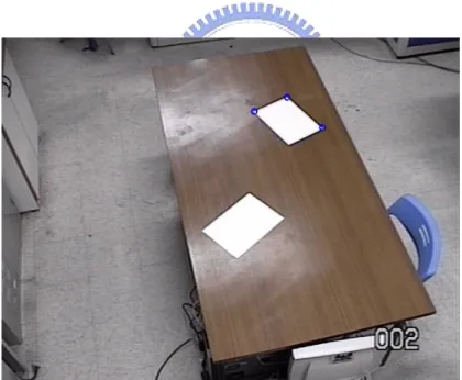
(24) unless we know the exact timing of camera’s movement and the sampling instant of each image frame. With multiple cameras, the synchronization problem becomes even more complicated. In this case, the use of pre-encoder may not offer instantaneous multi-view geometry information at any time instant. Hence, instead of the rotatory encoder, we seek to recalibrate a set of multiple cameras based on the feedback of visual information in the captured images. Up to now, various kinds of approaches have been developed to calibrate static camera’s intrinsic and/or extrinsic parameters, such as the techniques proposed in [1]-[43]. Nevertheless, it is impractical to repeatedly perform these elaborate calibration processes over a camera when the camera is under panning or tilting all the time. On the other hand, [9]-[11] have proposed plane-based calibration methods specially designed for the calibration of multiple cameras. However, for a wide-range surveillance system with multiple active cameras, these planar calibration objects may not be properly observed by all cameras when cameras are under movement. For dynamic camera calibration, some methods have been proposed in the literature [38]-[43]. However, they are not general enough to be applied in a wide-range surveillance system with multiple active cameras. Besides, [42] and [43] require the correspondence of feature points on the image pair. For surveillance systems with wide-range coverage, the matching of feature points is usually a difficult problem. In this thesis, we first demonstrate a new and efficient approach to calibrate multiple cameras without movement. For the static calibration, we estimate the tilt angle and altitude of each camera as a starting point. The concept of our approach originated from the observation that people could usually make a rough estimate about the tilt angle of the camera simply based on some clues revealed in the captured images. Based on our approach, once a set of cameras are settled, we can simply place a few simple patterns on a horizontal plane. These patterns can be A4 papers, books, 2.

(25) boxes, etc.; and the horizontal plane can be a tabletop or the ground plane. The whole procedure does not need specially designed calibration patterns. For example, with the image shown in Fig. 1.1, with the shape of the tabletop and these A4 papers on the table, we can easily infer that the camera has a pretty large tilt angle, which is expected to be larger than 45 degrees. Once the tilt angle and altitude of each camera are estimated, we will show that the relative positions and orientations among these cameras can be easily calibrated, without the need to calculate the homography matrix. It is worthwhile to mention that, in some sense, our approach can be thought to have decomposed the computation of homography matrix into two simple calibration processes so that the computational load becomes lighter for the calibration of multiple PTZ cameras.. Fig. 1.1. An example of images captured by a camera mounted on the ceiling.. So far as we know, most calibration algorithms require corresponding feature points, special calibration patterns, or known landmarks in the three dimensional space. To dynamically calibrate multiple cameras, calibration patterns and landmarks are not always applicable since they may get occluded or even move out of the 3.

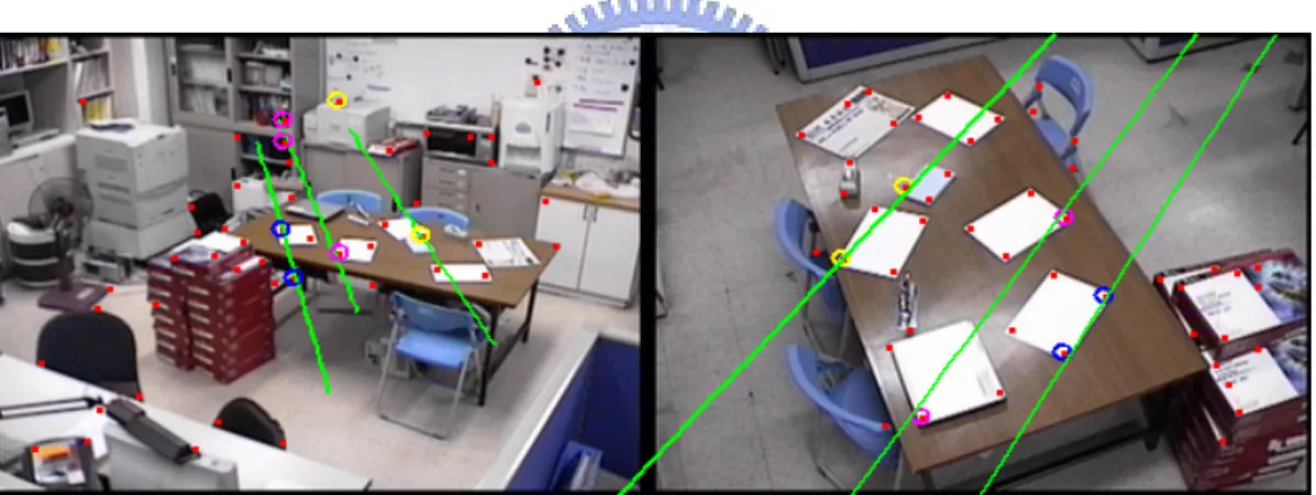
(26) captured scenes when cameras pan or tilt. On the other hand, if using the correspondence of feature points, we need to keep updating the correspondence of feature points when cameras rotate. For a wide-range surveillance system with many cameras, the correspondence of feature points cannot be easily solved. Take Fig. 1.2 as an example, the captured scenes of two cameras are quite different. We show three pairs of corresponding epipolar lines on these two images. It can be observed that feature points on each pair of corresponding epipolar lines may not originate from the same 3-D points. For this kind of image pair, the matching of feature points is not a simple task. Hence, after the static calibration of multiple cameras, we seek to recalibrate multiple cameras without specific calibration patterns and without complicated correspondence techniques.. Fig. 1.2. An image pair with two different views. Green lines indicate three pairs of. corresponding epipolar lines.. Based on the result of our static calibration of multiple cameras, we begin to perform dynamic calibration when the cameras are under movement. The concept of our approach originated from the observation that people can usually identify the directions of the pan and tilt angles, and even make a rough estimate about the changes of pan and tilt angles, simply based on some clues revealed in the captured images. The major advantage of our dynamic calibration algorithm is that it does not 4.

(27) require a complicated correspondence of feature points. As cameras begin to pan or tilt,. we. keep. extracting. and. tracking. feature. points. based. on. the. Kanade-Lucas-Tomasi (KLT) algorithm [45]. Next, we utilize the displacement of feature points and the epipolar-plane constraint among multiple cameras to infer the changes of pan and tilt angles for each camera. Compared with [42], we only need the correspondence of epipolar lines but not the exact matching of feature points. The use of epipolar lines greatly simplifies the correspondence process and makes our approach suitable for complicated surveillance environments. Our algorithm also allows the presence of moving objects in the captured scenes while performing dynamic calibration. This property makes our approach practical for general surveillance systems.. 1.2. Organization. The following chapters in this dissertation are organized as follows. . In Chapter 2, we first introduce the basic camera projection geometry, including the perspective projection, the epipolar geometry and the homography concept. Next, a few literatures are briefly reviewed.. . In Section 3.1, the camera model of our surveillance system is first described. Next, in Section 3.2, we develop the mapping between the 3-D space and the 2-D image plane in terms of tilt angle, under the constraint that all observed points are lying on a horizontal plane. Based on the back projection formula, the tilt angle and altitude of a camera can thus be estimated by viewing some simple patterns on a horizontal plane. Then, we will introduce how to utilize the estimation results to achieve the calibration of multiple cameras in Section 3.3. In addition, the sensitivity analysis with respect to parameter fluctuations and measurement errors will be discussed in Section 3.4. In Section 3.5, some 5.

(28) experimental results over real data are demonstrated to illustrate the feasibility of the proposed static calibration method. . In Section 4.1, based on the results of our static calibration, we explain how we utilize the displacement of feature points and the epipolar-plane constraint to infer the changes of pan angle and tilt angle. Then, in Section 4.2, we describe how to filter out undesired feature points when moving objects are present. After that, the sensitivity analysis with respect to measurement errors and the fluctuations of previous estimations will be addressed in Section 4.3. In Section 4.4, the efficiency and feasibility of this dynamic calibration approach are demonstrated in some experiments over real scenery.. . Finally, conclusions are drawn in Chapter 5.. 6.

(29) CHAPTER 2. Backgrounds ______________________________________________ To understand camera calibration, we start by briefly introducing the camera projection geometry that relates the world coordinate system with camera’s image coordinate system. In Section 2.1, the perspective projection commonly used for camera calibration will be introduced first. Next, we will show the geometric relationship of two views ⎯ the epipolar geometry and the homography. Then, in Section 2.2, we roughly classify some existing calibration methods [1]-[43] based on the usage of the calibration objects. Additionally, some dynamic calibration approaches are briefly introduced in Section 2.3.. 2.1. Projective Geometry. The commonly used camera model for camera calibration is the pinhole camera model, which is also called the perspective projection model. Although real cameras are usually equipped with lenses, the perspective projection model often approximates well enough to an acceptable camera projection process. In Section 2.1.1, we first 7.

(30) introduce the perspective projection and the camera parameters that relate the world coordinate system with the image coordinate system. Then, for multiple cameras, we extend our discussion to the two-view geometry, the epipolar geometry and the homography in Section 2.1.2 and Section 2.1.. 2.1.1. Perspective Projection. The pinhole perspective projection model was first proposed by Brunelleschi at the early 15th century [3, pp. 3-6], as illustrated in Fig. 2.1. For the sake of convenience, we consider a virtual image in front of the pinhole, instead of the inverted image behind the pinhole. The distances from this virtual image to the pinhole and from the pinhole to the actual image are the same. Figure 2.2 illustrates the perspective projection system [3, p. 28-30]. The origin O is the camera projection center (pinhole). The ray passing through the projection center and perpendicular to the image plane is called the optical axis. The optical axis interacts the image plane at the image center C. Assume P=[X, Y, Z]T denotes the world coordinates of a 3-D point P and its image coordinates are denoted as p= [x, y]T. Under perspective projection, we have. X X ⎧ ⎪⎪ x = kf Z = α Z , ⎨ ⎪ y = lf Y = β Y . ⎪⎩ Z Z. (2.1). Here, the image point is expressed in pixel units. The scale parameters k and l relate from a distance level to a pixel level. To simplify the equations, we replace kf and lf with α and β, respectively.. 8.

(31) Fig. 2.1 Pinhole imaging model [3, p. 4].. Fig. 2.2 Perspective projection coordinate system [3, p. 28].. Generally, the origin of the image coordinate system is not at the image center C but at the lower-left or upper-left corner C0. Hence, we add (u0, v0) in (2.2) to represent the principal point C in pixel units. ⎧ ⎪⎪ x = α ⎨ ⎪y = β ⎪⎩. X + u0 Z Y + v0 Z. (2.2). Moreover, due to the manufacturing errors, the two image axes may have an angle θ which is not equal to 90 degrees. This makes (2.2) to be X Y ⎧ ⎪⎪ x = α Z − α cot θ Z + u0 . ⎨ Y β ⎪y = + v0 ⎪⎩ sin θ Z 9. (2.3).

(32) These parameters α, β, u0, v0, and θ are called the intrinsic parameters of a camera. Usually, the perspective image plane will be moved to the front of the pinhole with a unit distance. For such a normalized coordinate system, the perspective projection can be expressed by ⎡α ⎢ ⎢ 1 p = [ K 0]P, where K = ⎢ 0 z ⎢ ⎢0 ⎣. −α cot θ. β sin θ 0. u0 ⎤ ⎥ ⎥ v0 ⎥ . ⎥ 1 ⎥⎦. (2.4). In (2.4), We reassume P=[X, Y, Z, 1]T denotes the homogeneous world coordinates of P and p= [x, y, 1]T denotes the homogeneous image coordinates of p’s perspective projection. Additionally, if the world coordinate system of P does not coincide with that in the camera projection system, the mapping between the image plane and the 3-D space becomes. p=. 1 K [R t ]P. z. (2.5). Here, R is a rotation matrix and t is a translation vector. They are called extrinsic parameters.. 2.1.2. Epipolar Geometry. Now considering a more complicated situation, we introduce the geometric relationship between two views of the same scene [3, p. 216-219]. We assume two cameras are observing the scenery. For these two cameras, their projection centers, O and O’, together with a 3-D point P, determine an epipolar plane ∏, as shown in Fig. 2.3. This epipolar plane ∏ intersects the image planes of the cameras to form two epipolar lines l and l’. The epipolar line l passes through the epipole e while l’ passes through e’. The epipole e is the projection of O’ observed by the first camera, while e’ 10.

(33) is the projection of O observed by the second cameras. If p and p’ are the projected points of P on these two image planes, they must lie on l and l’, respectively. This epipolar constraint implies that O, O’, p, and p’ are coplanar. For calibrated cameras with known intrinsic parameters, this constraint can be expressed as. JJJK JJJJK JJJJK Op ⋅ [OO′ × O′p′]=0.. (2.6). If we choose the first camera coordinate system as the reference coordinate system and consider the coordinate transformation of the second one, (2.6) can be rewritten as p ⋅[t × ( Rp′)] ≡ pT Ep′ = 0.. (2.7). Here, p and p’ are homogeneous image coordinate vectors, t is the translation JJJJK vector OO′ , and R is the rotation matrix. If a vector has the coordinates v’ in the second camera coordinate system, from the view of the first one, this vector has the coordinates v = Rv’. Moreover, E = t × R is called the essential matrix [3, p. 217]. By (2.7), Ep’ and ETp can be interpreted as the homogeneous coordinates of the epipolar lines l and l’ in terms of the image points p and p’, respectively.. Fig. 2.3 Illustration of epipolar-plane constraint. Furthermore, when we consider the intrinsic parameters of these two cameras, based on (2.4), the world coordinates of P observed by the first camera (second. 11.

(34) camera) can be represented by K-1p (K’-1p’) up to a scale. In this way, (2.7) is rewritten as pT K −T EK ′−1 p′ ≡ pT Fp′ = 0.. (2.8). Equation (2.8) is called the Longuet-Higgins equation and F is called the fundamental matrix [3, pp. 218-219]. Similar to E, Fp’ and FTp can be interpreted as the epipolar line l and l’, respectively. Therefore, F can be considered as the mapping from an image point on one view to the epipolar line on the other view. The epipolar constraint plays an important role and is often used in the camera calibration. Based on the information of the point correspondence among multiple views of image frames, we may extract the intrinsic parameter K or/and the extrinsic parameters R and t.. 2.1.3. Homography. Because a homography is often used to calibrate multiple views of cameras, we also briefly describe it here. We will also introduce the combination of the epipolar constraint and homography [44, pp. 325-343].. Fig. 2.4 A homography between two views [44, p. 325]. 12.

(35) As shown in Fig. 2.4, a homography HΠ that is induced by a plane Π in the 3-D space can map the image points p and p’ between two views. To be more apprehensible, through the transformation H2Π, we first back-project the image point p’ on the second frame to the space point PΠ on the plane Π. Then, PΠ is projected to. the image point p on the first frame by the transformation H1Π. This procedure can be expressed as p = H1Π H 2−Π1 p′ = H Π p′.. (2.9). In theory, the 3×3 matrix HΠ can be obtained by four image point correspondences between two views. However, a homography needs to conform to the epipolar constraint so that the mapping of the two image planes can obey the projective geometry.. Fig. 2.5 A homography compatible with the epipolar geometry [44, pp. 328].. Figure 2.5 shows the projective geometry combining a homography induced by a plane Π and the epipolar plane constraint. In the homogeneous forms, the epipolar line l can be represented by l = e × p = [e]× ( H Π p′).. (2.10). As mentioned in Section 2.1.2, the epipolar constraint related with one image point on 13.

(36) one view and one epipolar line on the other view can be expressed as l = Fp’. Combining this constraint with (2.10), we can obtain F = [e]× H Π .. (2.11). This formula is illustrated in Fig. 2.6.. Fig. 2.6 The fundamental matrix can be represented by F = [e]× H Π , where H Π is the projective transform from the second to the first camera, and [e]× represents the fundamental matrix of the translation [44, p. 250].. Here, we simply mention the concept of a homography and add the epipolar constraint on it. Some papers [7], [10], [11], [14]-[36] have developed their camera calibration methods based on this compatibility constraint.. 14.

(37) 2.2. Camera Calibration. Up to now, plenty of camera calibration methods have already been developed in the literature [1]-[36]. According to their calibration objects, these methods can be roughly classified into four categories: calibration with three-dimensional objects, calibration with planar objects, calibration with one-dimensional objects, and self-calibration (with no specific objects). These methods will be briefly introduced in Section 2.2.1- 2.2.4.. 2.2.1. Calibration with Three-Dimensional Objects. This type of calibration methods [1]-[3, pp. 38–53] uses 3-D objects or 3-D reference points with known world coordinates to calibrate cameras. Among these methods, O. Faugeras [2] proposed an approach that uses the calibration pattern as shown in Fig. 2.7. Such a calibration object usually contains two or three planes orthogonal to each other so that the object forms a reference world coordinate system. Some regularly arranged rectangles are on these planes. In this way, the coordinates of the corner on these rectangles are exactly known. Based on these reference correspondences between the world coordinate system and the image coordinate system, the projective map M which is called the camera matrix can be obtained by minimizing the geometric distance errors as follows:. ∑ d ( p , pˆ ) i. i. 2. .. (2.12). i. In (2.12), i is the number of corresponding points, and pˆ i = MPi . Finally, the intrinsic and extrinsic parameters can be estimated by decomposing M. Beside this approach, [1] uses different sets of 3-D reference points for calibration, while [3] offers some other optimization processes to estimate the intrinsic and extrinsic parameters.. 15.

(38) Basically, these approaches tried to build the mapping between the 3-D coordinate system and the image coordinate system. In summary, these methods based on 3-D reference points usually need special set-ups. Moreover, they can hardly be applied to the calibration of multiple cameras since the 3-D calibration object has to be in the view of all cameras. Especially, for dynamic calibration, it is even more difficult to calibrate cameras based on these methods. Fig. 2.7 A 3-D calibration pattern with regularly arranged rectangles.. 2.2.2. Calibration with Planar Objects. Since planar objects can usually be observed in the scene and are easier to be patched with some specific geometric features, some calibration methods [4]-[11] have been proposed by using planar calibration objects. Compared with the 3-D calibration objects, planar objects are more suitable for the calibration of multiple cameras [8]-[11].. 16.

(39) In principle, the majority of these plane-based calibration methods built the homography between a viewed plane in the 3-D space and its projection on the image plane. Based on sufficient point correspondences, this homography can be estimated. Furthermore, by changing the rotation and translation of this calibration plane several times, we have several homographies, where the same camera intrinsic parameters are embedded. From these homographies, the intrinsic parameters can be extracted by applying some constraints. The differences among different methods lie on the adopted conditions, such as a known structure of planar features or a known external motion of the calibration plane. We take [4] as an example, due to its flexibility and easier implementation. Under perspective projection, based on (2.5), the principle procedure mentioned above can be formulized by ⎡X ⎤ ⎡X ⎤ ⎢ ⎥ t ] ⎢ Y ⎥ = H ⎢⎢ Y ⎥⎥ , ⎢⎣ 1 ⎥⎦ ⎢⎣ 1 ⎥⎦. λ p = K [R t ]P = K [r1 r2. (2.13). where λ is an arbitrary scale factor; and r1 and r2 are the first two column vectors of the rotation matrix R. Note that because P is on a plane, its coordinates can be simplified to be [X, Y, 1]T without loss of generality. In addition, from the fact that r1 and r2 are orthogonal to each other, the other two constraints of the homography and the intrinsic parameters can be obtained as h1T K −T K −1h2 = 0 and. (2.14). h1T K −T K −1h1 = h2T K −T K −1h2 .. (2.15). In (2.14) and (2.15), h1, h2, and h3 are the three column vectors of H. However, there are 6 extrinsic parameters, 3 for rotation and 3 for translation; while a homography has 8 degrees of freedom. Having one homography provides only two constraints on. 17.

(40) the intrinsic parameters. Hence, we need at least three different views to solve 6 intrinsic parameters. In [4], an additional parameter, lens distortion, was considered. Other plane-based methods [8]-[11] have been specially designed for the calibration of multiple cameras. The work in [8] calibrates the intrinsic parameters with a planar grid first. Then, relative to a reference grid on the floor, the position of each camera is estimated. However, this method needs to take several image views to complete the calibration task. In comparison, [9] needs fewer views. In [9], the proposed process is like an integration of static camera calibration and “moving” camera calibration. It needs a multi-camera rig to change the specific orientation of cameras to capture two or more views of a calibration grid. With such a known condition of camera motion, this approach needs at least two views to recover the fixed intrinsic parameters and the extrinsic parameters of cameras. On the other hand, the approaches proposed in [10] and [11] belong to factorization-based methods. In [10], the cameras are assumed to be well calibrated beforehand. The author recovered the poses of multiple planes and multiple views relative to a global 3-D world reference frame by using coplanar points with known Euclidean structure. The method in [11] is an extension of [7]. Both intrinsic and extrinsic parameters can be estimated via factorization of homography matrices. However, for surveillance systems with multiple cameras, these elaborate processes and the adopted constraints do not seem to be practical choices. Even though such 2-D calibration objects are simpler than the 3-D calibration object mentioned in Section 2.2.1, specific planar calibration objects with known structure are still needed to achieve the calibration task. As the number of cameras increases, or for wide-range multi-camera systems, a planar object may not be simultaneously observed by all cameras. Thereafter, more calibration objects are needed and more image frames need be captured to complete the calibration process. Besides, for 18.

(41) dynamic calibration, it is not an efficient way to repeatedly adopt these methods to recalibrate cameras.. 2.2.3. Calibration with One-Dimensional Objects. Recently, Zhang [12] proposed a camera calibration method that used a one-dimensional object with three points on it. The length of this object L and the relative positions between these points are known in advance. In addition, one of these points is fixed in the 3-D space. The camera imaging system of these collinear space points A, B, and C is illustrated in Fig. 2.8. With these constraints, some equations are deduced as follows. B − A = L2. 2. (2.16). C = λ A A + λB B. (2.17). Based on (2.5), when [R t] were chosen as [I 0], the following equation is obtained. A = z A K −1a, B = z B K −1b, and C = zC K −1c. (2.18). In (2.18), zA, zB, and zC are the unknown depths of A, B, and C, respectively. Based on (2.18), (2.17) is rewritten as zC c = z Aλ Aa + zB λB b. (2.19). By applying cross-product with c on (2.19), (2.20) is obtained. z AλA (a × c) + zB λB (b × c) = 0. (2.20). Finally, based on (2.16), (2.18) and (2.20), a basic camera calibration constraint by using a 1-D object is obtained as follows. z A2 hT K −T K −1h = L2 .. In (2.21), h = a +. (2.21). λA (a × c) ⋅ (b × c) b. Hence, with the known length of the calibration λB (b × c) ⋅ (b × c). bar, the known position of the point C with respect to A and B, and a fixed point A,. 19.

(42) the 5 intrinsic parameters of the camera together with zA can be estimated by using at least six different views of the calibration bar. Such a calibration operation with a fixed space point is shown in Fig. 2.9. A more detailed discussion of this calibration method can be found in [13].. Fig. 2.8 Camera imaging system of a one-dimensional object [12].. Fig. 2.9 An example of the calibration operation by using a 1-D object with a fixed point [12].. Since a 1-D object with known geometry is easy to be constructed and is more likely to be observed by multiple cameras at the same time, this calibration method seems to be potentially suitable for the calibration of multiple cameras. However, during the calibration, it still needs manual operations. That is, we need to fix a 3-D 20.

(43) point and change the direction of the calibration stick. Otherwise, a special calibration pattern will be required. For active cameras that may change their poses from time to time, such a technique does not seem to be a practical choice either.. 2.2.4. Self-Calibration. Several research works about self-calibration [14]-[37] have been done in the last decade. The theory of self-calibration was first introduced by Maybank and Faugeras [14]. Very different from the aforementioned calibration methods, self-calibration methods do not require either calibration objects with known structure or the motion information of a camera. Based on the epipolar constraint produced by the displacement of an uncalibrated camera, the camera can be calibrated via the absolute conic Ω. Here, we briefly describe the major kind of self-calibration techniques. The absolute conic is defined to be a conic of purely imaginary points on the plane at infinity. It can be expressed as X 12 + X 22 + X 32 ⎫⎪ ⎬ = 0, X 4 ⎪⎭ ( X 1 , X 2 , X 3 )Ω( X 1 , X 2 , X 3 )T = 0,. (2.22). where Ω = I.. The absolute conic has an important property that its image ω is invariant under rigid motions of a camera. Under perspective projection, the dual matrix of ω can be represented by ω ∗ = KK T . Figure 2.10 shows the epipolar constraints of ω between two image frames. The first camera constraint is that the epipolar line l = e×p is tangent to ω if and only if (e × p)T ω ∗ (e × p) = 0.. (2.23). The second camera constraint is that the epipolar line l’ = Fp represented by the 21.

(44) corresponding point p on the first image and the fundamental matrix F is tangent to ω’ if and only if pT F T ω ′∗ Fp = 0.. (2.24). Equations (2.23) and (2.24) are the so-called Kruppa equations [37]. If the intrinsic parameters are constant, (2.23) and (2.24) can be further combined into (2.25). [e]× ω ∗[e]× = F T ω ∗ F .. (2.25). From at least three different views where each F can be obtained based on point correspondences between two views, the intrinsic parameters of the camera can be extracted.. Fig. 2.10 The epipolar tangency to the absolute conic images [18].. In fact, self-calibration techniques are mainly concerned with the intrinsic parameters of cameras. Most self-calibration approaches [14]-[26] were proposed 22.

(45) concerning constant intrinsic parameters. Among these methods, [22]-[26] solve their problem with additional camera motion restrictions. On the other hand, much extended research [27]-[35] has been developed to solve varying intrinsic parameters. Some of them [31]-[35] additionally utilize camera motion constraints to achieve calibration work. The further detail discussions of camera self-calibration approaches can be found in [36]. Although self-calibration has no or fewer assumptions about the camera motion information and doesn’t require specific calibration objects, the computational load is heavy and the calibration work is too elaborate to be applied to the dynamic calibration of multiple cameras.. 23.

(46) 2.3. Dynamic Camera Calibration. Up to now, very few research works [38]-[43] have been proposed for dynamic camera calibration. Most existing dynamic calibration techniques concern with extrinsic parameters of cameras. Jain et al [38] proposed an off-line method, where they tried to find the relationship between the realized rotation angle and the requested angle. In [39], the pose of a calibrated camera is estimated from a planar target. However, both [38] and [39] only demonstrate the dynamic calibration of a single camera, but not the calibration among multiple cameras. In [40], the authors utilize the marks and width of parallel lanes to calibrate PTZ cameras. In [41], the focal length and two external rotations are dynamically estimated by using parallel lanes. Although these two methods are practical for traffic monitoring, it is not general enough for other types of surveillance systems. In [42], a dynamic camera calibration with narrow-range coverage was proposed. For a pair of cameras, this method performs the correspondence of feature points on the image pair and uses coplanar geometry for camera calibration. In [43], the relative pose between a calibrated camera and a projector is determined via plane-based homography. The authors took two steps to recalibrate the pose parameters. They first estimated the translation vector and then found the rotation matrix. They also offered analytic solutions. Nevertheless, this approach requires the correspondence of feature points. So far as we know, most calibration algorithms require corresponding feature points, special calibration patterns (coplanar points with known structure or parallel lines), or known landmarks in the three dimensional space. However, to dynamically calibrate multiple cameras, calibration patterns and landmarks are not always applicable since they may get occluded or even are out of the captured scenes when cameras pan or tilt. On the other hand, in the correspondence of feature points, we. 24.

(47) need to keep updating the correspondence of feature points when cameras rotate. For surveillance systems with a wide-range coverage, the matching of feature points is usually a difficult problem. Hence, in this thesis, we develop a new algorithm for the dynamic calibration of multiple cameras, without the need of a complicated correspondence of feature points.. 25.

(48) 26.

(49) CHAPTER 3. Static Calibration of Multiple Cameras ______________________________________________ I In this chapter, we introduce how to efficiently calibrate the extrinsic parameters of multiple static cameras. In Section 3.1, the camera model of our surveillance system is first described. Next, in Section 3.2, we will deduce the 3D-to-2D coordinate transformation in terms of the tilt angle of a camera. In [46], a similar scene model based on pan angle and tilt angle has also been established. In this paper, however, we will deduce a more complete formula that takes into account not only the translation effect but also the rotation effect when a camera is under a tilt movement. After having established the 3D-to-2D transformation, the tilt angle and altitude of a camera can thus be estimated based on the observation of some simple objects lying on a horizontal plane. Then, we will introduce how to utilize the estimation results to achieve the calibration of multiple cameras in Section 3.3. In addition, the sensitivity analysis with respect to parameter fluctuations and measurement errors will be 27.

(50) discussed in Section 3.4. In Section 3.5, some experimental results over real data are demonstrated to illustrate the feasibility of the proposed static calibration method.. 3.1. Introduction of Our Camera Model System. In this section, we give a sketch of our system overview, camera setup model and the basic camera projection model. Although the camera model is built based on our surveillance environment, this model is general enough to fit for a large class of surveillance scenes, which are equipped with multiple cameras.. 3.1.1. System Overview. In the setup of our indoor surveillance system, four PTZ cameras are mounted on the four corners of the ceiling in our lab, about 3 meters above the ground plane. The lab is full of desks, chairs, PC computers, and monitors. All the tabletops are roughly parallel to the ground plane. These cameras are allowed to pan or tilt while they are monitoring the activities in the room. Figure 3.14(a) shows four images captured by these four cameras. We will first estimate the tilt angle and altitude of each camera based on the captured images of some prominent features, such as corners or line segments, on a horizontal plane. Once the tilt angles and altitudes of these four cameras are individually estimated, we will perform the calibration of multiple cameras. Figure 3.1 shows the flowchart of the proposed static calibration procedure.. 28.

(51) Fig. 3.1 Flowchart of the proposed static calibration procedure.. 3.1.2. Camera Setup Model. Figure 3.2 illustrates the modeling of our camera setup. Here, we assume the observed objects are located on a horizontal plane ∏, while the camera lies above ∏ with a height h. The camera may pan or tilt with respect to the rotation center OR. Moreover, we assume the projection center of the camera, denoted as OC, is away from OR with distance r. To simplify the following deductions, we define the origin of the rectified world coordinates to be the projection center OC of a camera with zero tilt angle. The Z-axis of the world coordinates is along the optical axis of the camera, while the Xand Y-axis of the world coordinates are parallel to the x- and y-axis of the projected image plane, respectively. When the camera tilts, the projection center moves to OC’ and the projected image plane is changed to a new 2-D plane. In this case, the y-axis of the image plane is no longer parallel to the Y-axis of the world coordinates, while the x-axis is still parallel to the X-axis. Assume P=[X, Y, Z, 1]T denotes the homogeneous coordinates of a 3-D point P in the world coordinates. For the case of a camera with zero tilt angle, we denote the perspective projection of P as p= [x, y, 1]T. Under perspective projection, the. 29.

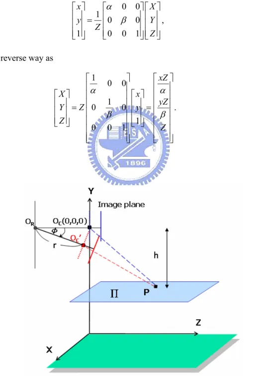
(52) relationship between P and p can be expressed as Equation (2.5), p =. 1 K [R t ]P. z. With respect to the rectified world coordinate system, the extrinsic term [R t] becomes [I 0]. To further simplify the mathematical deduction, we ignore the skew angle and assume the image coordinates have been translated by a translation vector (-u0, -v0). Hence, (2.5) can be simplified as. ⎡ x⎤ ⎡α ⎢ y⎥ = 1 ⎢ 0 ⎢ ⎥ Z⎢ ⎢⎣ 1 ⎥⎦ ⎢⎣ 0. 0⎤ ⎡ X ⎤ 0⎥⎥ ⎢⎢ Y ⎥⎥ , 1 ⎥⎦ ⎢⎣ Z ⎥⎦. (3.1). ⎤ ⎡ xZ ⎤ 0⎥ ⎢α ⎥ ⎥ ⎡ x⎤ ⎢ ⎥ yZ 0⎥ ⎢⎢ y ⎥⎥ = ⎢ ⎥ . ⎥ ⎢β ⎥ ⎥ ⎢1⎥ ⎢ ⎥ 1⎥ ⎣ ⎦ ⎢ Z ⎥ ⎦⎥ ⎣⎢ ⎦⎥. (3.2). 0. β 0. or in a reverse way as ⎡1 ⎢α ⎡X ⎤ ⎢ ⎢Y ⎥ = Z ⎢ 0 ⎢ ⎥ ⎢ ⎢⎣ Z ⎥⎦ ⎢ ⎢0 ⎣⎢. 0 1. β 0. Fig. 3.2 Model of camera setup. 30.

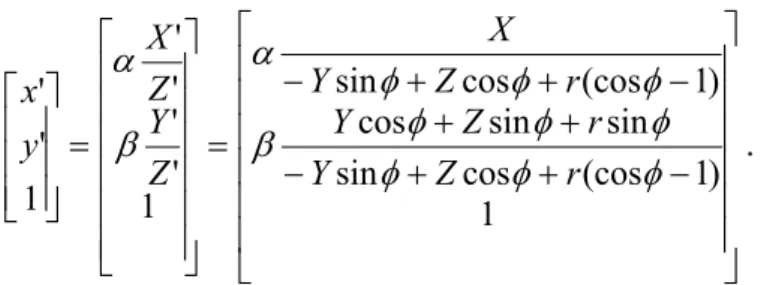
(53) 3.2. Pose Estimation of a Single Camera. In this section, we first deduce the projection equation to relate the world coordinates of a 3-D point p to its image coordinates on a tilted camera. Then, under the constraint that all observed points are located on a horizontal plane, the mapping between the 3-D space and the 2-D image plane is further developed. Finally, we deduce the formulae for the pose estimation of a camera.. 3.2.1. Coordinate Mapping on a Tilted Camera. When the PTZ camera tilts with an angle φ, the projection center OC translates to a new place OC’ with OC’ =[0 -rsinφ -(r-rcosφ)]T. Assume we define a tilted world coordinate system (X’, Y’, Z’) with respect to the tilted camera, with the origin being the new project center OC’, the Z’-axis being the optical axis of the tilted camera, and the X’- and Y’-axis being parallel to the x’- and y’-axis of the new projected image plane, respectively. Then, it can be easily deduced that in the tilted world coordinate system the coordinates of the 3-D point P become. 0 0 ⎤⎡ X ⎡ X ′⎤ ⎡1 ⎤ ⎢ Y ′ ⎥ = ⎢0 cos φ sin φ ⎥ ⎢ Y + r sin φ ⎥ ⎢ ⎥ ⎢ ⎥⎢ ⎥ ⎢⎣ Z ′ ⎥⎦ ⎢⎣0 − sin φ cos φ ⎥⎦ ⎢⎣ Z + r (1 − cos φ ) ⎥⎦ X ⎡ ⎤ ⎢ = ⎢ Y cos φ + Z sin φ + r sin φ ⎥⎥ . ⎢⎣ −Y sin φ + Z cos φ + r (cos φ − 1) ⎥⎦. (3.3). After applying the perspective projection formula, we know that the homogeneous coordinates of the projected image point now move to. 31.

(54) ⎡ x'⎤ ⎢ y '⎥ ⎢ ⎥ ⎢⎣ 1 ⎥⎦. 3.2.2. X ⎤ ⎡ X ' ⎤ ⎡α α ⎢ ⎢ Z' ⎥ − Y sin φ + Z cosφ + r (cosφ − 1) ⎥ ⎢ ⎥ ⎢ Y' ⎥ Y cosφ + Z sin φ + r sin φ ⎢ ⎥. = ⎢β ⎥ = β ⎢ Z ' ⎥ ⎢ − Y sin φ + Z cosφ + r (cosφ − 1) ⎥ ⎥ ⎢ 1 ⎥ ⎢ 1 ⎥ ⎥⎦ ⎢ ⎢⎣ ⎣ ⎦. (3.4). Constrained Coordinate Mapping. In the rectified world coordinates, all points on a horizontal plane have the same Y coordinate. That is, Y = -h for a constant h. The homogeneous form of this plane ∏ can be defined as π = [0 1 0 h]T . Assume the camera is tilted with an angle φ. Then, in the tilted world coordinate system, the homogeneous form of this plane ∏ becomes π ′ = [0 cos φ. − sin φ. (h − r sin φ )]T , as shown in Fig. 3.3.. Fig. 3.3 Geometry of a horizontal plane ∏ with respect to a tilted camera.. Assume a 3-D point p is located on the horizontal plane ∏. Then, in the rectified world coordinate system, we have π ⋅ P = 0 , where P = [X, Y, Z, 1]T. Similarly, in the tilted world coordinate system, we have π ′ ⋅ P′ = 0 , where P’ = [X’, Y’, Z’, 1]T. With (3.2), Z’ can be found to be. 32.

(55) Z′ =. β ( r sin φ − h) . y ′ cos φ − β sin φ. (3.5). Moreover, the tilted world coordinates of p become. ⎡ x′β (r sin φ − h) ⎤ ⎢ α ( y′ cos φ − β sin φ ) ⎥ ⎥ ⎡ X ′⎤ ⎢ ′ ⎢ ⎥ − φ ( sin ) y r h ⎢Y′ ⎥ = . ⎢ ⎢ ⎥ ′ cos φ − β sin φ ⎥ y ⎥ ⎢⎣ Z ′ ⎥⎦ ⎢ ⎢ β (r sin φ − h) ⎥ ⎢ ′ ⎥ ⎣ y cos φ − β sin φ ⎦. (3.6). With (3.3) and (3.6), we may transfer [X’, Y’, Z’]T back to [X, Y, Z]T to obtain. x′β (r sin φ − h) ⎡ ⎤ ⎢ ⎥ α ( y′ cos φ − β sin φ ) ⎡X ⎤ ⎢ ⎥ ⎢Y ⎥ = h . − ⎢ ⎥ ⎢ ⎥ ⎢ ⎥ ′ ⎢⎣ Z ⎥⎦ ⎢ ( y sin φ + β cos φ )(r sin φ − h) − r + r cos φ ⎥ y′ cos φ − β sin φ ⎢⎣ ⎥⎦. (3.7). If the principal point (u0, v0) is taken into account, then (3.7) can be reformulated as. ( x′ − u0 ) β ( r sin φ − h) ⎡ ⎤ ⎢ ⎥ ′ α [(v0 − y ) cos φ − β sin φ ] ⎡X ⎤ ⎢ ⎥ ⎢Y ⎥ = ⎢ ⎥. − h ⎢ ⎥ ⎢ ⎥ ⎢⎣ Z ⎥⎦ ⎢ [(v0 − y′) sin φ + β cos φ ](r sin φ − h) − r + r cos φ ⎥ ⎢⎣ ⎥⎦ (v0 − y′) cos φ − β sin φ. (3.8). This formula indicates the back projection formula from the image coordinates of a tilted camera to the rectified world coordinates, under the constraint that all the observed points are lying on a horizontal plane with Y = -h.. 33.

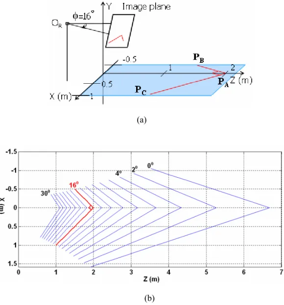
(56) 3.2.3. Pose Estimation Based on the Back-Projections. As aforementioned, in real life, based on the image contents of a captured image, people can usually have a rough estimate about the relative position of the camera with respect to the captured objects. In this section, we demonstrate that, with a few corners or a few line segments lying on a horizontal plane, we can easily estimate the tilt angle of the camera based on the back projection of the captured image.. 3.2.3.1. Back-projected Angle w.r.t. Guessed Tilt Angle. Suppose we use a tilted camera to capture the image of a corner, which is located on a horizontal plane. Based on the captured image and a guessed tilt angle, we may use (3.8) to back-project the captured image onto a horizontal plane on Y = -h. Assume three 3-D points, PA, PB, and PC, on a horizontal plane form a rectangular corner at PA. The original image is captured by a camera with φ = 16 degrees, as shown in Fig. 3.4(a). In Fig. 3.4(b), we plot the back-projected images for various choices of tilt angles. The guessed tilt angles range from 0 to 30 degrees, with a 2-degree step. The back-projection for the choice of 16o is plotted in red, specifically. It can be seen that the back-projected corner becomes a rectangular corner only if the guessed tilt angle is correct. Besides, it is worth mentioning that a different choice of h only causes a scaling effect of the back-projected shape. To formulate this example, we express the angle ψ at PA as. cosψ =. PA PB , PA PC PA PB × PA PC. .. (3.9). After capturing the image of these three points, we can use (3.8) to build the relation between the back-projected angle and the guessed tilt angle.. 34.

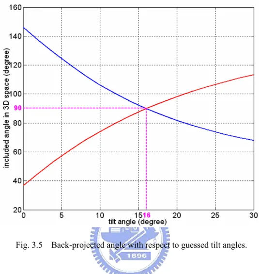
(57) xB′ β x′A β − ) α ( y′B cos φ − β sin φ ) α ( y′A cos φ − β sin φ ) xC′ β x′A β ×( − ) α ( yC′ cos φ − β sin φ ) α ( y′A cos φ − β sin φ ) ( y′ sin φ + β cos φ ) ( y′A sin φ + β cos φ ) ) +( B − yB′ cos φ − β sin φ y′A cos φ − β sin φ ( y′ sin φ + β cos φ ) ( y′A sin φ + β cos φ ) − )} ×( C yC′ cos φ − β sin φ y′A cos φ − β sin φ xB′ β x′A β )2 × {( − ′ ′ α ( yB cos φ − β sin φ ) α ( y A cos φ − β sin φ ) ( y′ sin φ + β cos φ ) ( y′A sin φ + β cos φ ) 2 − 12 )} +( B − yB′ cos φ − β sin φ y′A cos φ − β sin φ xC′ β x′A β × {( − )2 α ( yC′ cos φ − β sin φ ) α ( y′A cos φ − β sin φ ) ( y′ sin φ + β cos φ ) ( y′A sin φ + β cos φ ) 2 − 12 +( C − )} } yC′ cos φ − β sin φ y′A cos φ − β sin φ. ψ = cos −1{{(. (3.10). Note that in (3.10) we have ignored the offset terms, u0 and v0, to reduce the complexity of the formulation. In Fig. 3.5, we show the back-projected angle ψ with respect to the guessed tilt angle, assuming α and β are known in advance. In this simulation, the red and blue curves are generated by placing the rectangular corner on two different places of the horizontal plane. Again, the back-projected angle is equal to 90 degrees only if we choose the tilt angle to be 16 degrees. This simulation demonstrates that if we know in advance the angle of the captured corner, we can easily deduce camera’s tilt angle. Moreover, the red curve and the blue curve intersect at (φ, ψ) = (16 , 90). This means that if we don’t know in advance the actual angle of the corner, we can simply place that corner on more than two different places of the horizontal plane. Then, based on the intersection of the deduced ψ-v.s.-φ curves, we may not only estimate the tilt angle of the camera but also the actual angle of the corner.. 35.

(58) (a). (b) Fig. 3.4. (a) Rectangular corner captured by a tilted camera (b) Illustration of. back-projection onto a horizontal plane on for different choices of tilt angles.. 36.

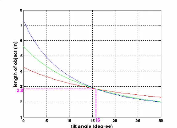
(59) Fig. 3.5 Back-projected angle with respect to guessed tilt angles.. 3.2.3.2. Back-projected Length w.r.t. Guessed Tilt Angle. Assume two 3-D points, PA and PB, on a horizontal plane form a line segment with length L. Similarly, we can build a similar relationship between the back-projected length and the guessed tilt angle by setting the constraint: PA PB = L. Based on this constraint and (3.8), we can deduce that. ( xB′ − u0 ) β (r sin φ − h) α [(v0 − yB′ ) cos φ − β sin φ ] ( x′A − u0 ) β (r sin φ − h) 2 ) − α [(v0 − y′A ) cos φ − β sin φ ] [(v − yB′ ) sin φ + β cos φ ](r sin φ − h) +( 0 (v0 − yB′ ) cos φ − β sin φ [(v − y′A ) sin φ + β cos φ ](r sin φ − h) 2 12 )} . − 0 (v0 − y′A ) cos φ − β sin φ. L = A(φ ) = {(. 37. (3.11).

(60) Similarly, if α, β, r, and h are known in advance, we can deduce the tilt angle directly based on the projected value of L. Note that in (3.11), the right-side terms contain a common factor (rsinφ-h)2. This means the values of r and h only affect the scaling of L. Hence, we can rewrite the formula of the L-v.s.-φ curve as L' ≡. L r sin φ − h. ⎛ ⎞ ( xB′ − u0 ) β ( x′A − u0 ) β = {⎜ − ⎟ ⎝ α [(v0 − y′B ) cos φ − β sin φ ] α [(v0 − y′A ) cos φ − β sin φ ] ⎠. 2. (3.12). 2. ⎛ [(v0 − yB′ ) sin φ + β cos φ ] [(v0 − y′A ) sin φ + β cos φ ] ⎞ 12 +⎜ − ⎟} . (v0 − y′A ) cos φ − β sin φ ⎠ ⎝ (v0 − yB′ ) cos φ − β sin φ. Then, even if the values of r and h are unknown, we may simply place more than two line segments of the same length on different places of a horizontal plane and seek to find the intersection of these corresponding L-v.s.-φ curves, as shown in Fig. 3.6.. 38.

(61) Fig. 3.6 Back-projected length with respect to guessed tilt angle. Each curve is generated by placing a line segment on some place of a horizontal plane.. As mentioned above, the tilt angle can be easily estimated from the ψ-v.s.-φ curves or L-v.s.-φ curves. However, in practice, due to errors in the estimation of camera parameters and errors in the measurement of (x’, y’) coordinates, the deduced ψ-v.s.-φ curves or L-v.s.-φ curves do not intersect at a single point. Hence, we may also seek to perform parameter estimation based on an optimization process. Here, we take (3.11) as an example. We assume several line segments with known lengths (not necessary of the same length) are placed on different positions of a horizontal plane and we use a tilted camera to capture the image. Assume the length of the ith segment is Li, then we aim to find a set of parameters {α, β, u0, v0, φ, r, h} that minimize. F ( x1′, y1′, x2′ , y2′ ,..., xm′ , ym′ , α , β , u0 , v0 , φ , r , h) m. = ∑ A i ( xi′, yi′, α , β , u0 , v0 , φ , r , h) − Li . 2. i =1. 39. (3.13).