d
d
d d
d
d d
d
d d
d
d d
d
d d
d
d
d
d
dd
d
dd
d
dd
d
dd
d
dd
d
dd
d
dd
d
dd
d
dd
d
d
d
d
d d
d
d d
d
d d
d
d
d
d
dd
d
dd
d
dd
d
dd
d
dd
d
dd
d
dd
d
dd
d
dd
d
dd
d
dd
d
dd
d
dd
d
dd
d
d
A Multiple-Instance Neural Networks for Content-based Image
Retrieval
d d ddd d d
dddddd d d
d
d
dd
d
dd
d
dd
d
dd
d
dd
d
dd
d
dd
d
dd
d
dd
d
dd
d
dd
d
dd
d
dd
d
dd
d
d
A Multiple-Instance Neural Networks for
Content-based Image Retrieval
d d ddd d d Student: Shun-Chin Chuang dddddd d d dd Advisor: Professor Hsin-Chia Fu
d d d d d d
d d d d
d d d d d d d d d d
d d d d
A Dissertation
Submitted to Department of Computer Science College of Computer Science
National Chiao Tung University in Partial Fulfillment of the Requirements
For the Degree of Doctor of Philosophy
in
Computer Science July 2010
Hsinchu, Taiwan, R.O.C.
d
d
dd
d
dd
d
dd
d
d
dddddddddddddddddddddddddddddddddddd dddddddddddddddddddddddddddddddddddddd dddddddddddddddddddddddddddddddddddddd ddddddddd ddddddddddddddddddddddddddddddddddd dMINNdd ddddddddddddddddddddddddddddddd ddddddd(1).dddddddddWeighted Color Histogramdd (2).ddddd ddddWeighted Texture Histogramddddddddddddddddddddd ddddddddddddddddddddddddddddddddd dddd ddddddddddddRegion of Interestingddd R.O.I.ddddddddddd ddddddddinstancedddddddddddddddddddddddddd dGaussian-like maskdddLABdddddddddddddddddddddddd dddddddddddddddddddddddddddddddddddddd dddddddddddddddddddddddddddddddddddddd dddddddddd ddddddddddddddddddddddddddddddddddddd dddddddddddddddd ddddddddModel Selectionddddddd dddddddddddddddddddddddddddddddddddddd ddWeighted BootstrapdddddddddddEmpiricaldddddddddddd ddddddddddddd MINN ddddddddd IRM [1] d UFM [2] ddddddd dd COREL gallery ddddddddd 100 dddddd MINN ddddddd dd(1).ddddddddddd dd (2).dddddddddddddddddd dddddd MINN ddddddddddddddddddddd
Abstract
In this dissertation, we proposed a novel Multiple-Instance Neural Networks (MINN) image content-based retrieval system. Due to the segmenting an image into regions au-tomatically is still a difficult task in image processing research, the proposed system can reduce the image retrieval problem to the multiple-instance problem in order to represent the content of an image without precisely image segmentation.
To tackle the multiple-instance based image retrieval problem, a statistical based Multiple-Instance Neural Networks (MINN) is proposed to approximate the true distribution of the query images in a more precise way than the previous approaches. Two novel image repre-sentation methods are proposed : (1) the Weighted Color Histogram and (2) the Weighted Texture Histogram. Features used in MINN image content-based retrieval system are the the parameters of mixture density functions which approximate the two histograms of im-ages in the Lab color space in each instance sampled by a Gaussian-like mask, and the measurement of a distance between two distributions is proposed.
In the process of approximating the histograms, how to determine the proper number of the clusters in the mixture Gaussian model of each class, that is, a problem about the model selection, is still an important issue. The weighted bootstrap method is proposed to make the selection more correctly.
Some experiments for the MINN are exercised and results shown that the proposed MINN is successful to learn the user’s visual concept more precisely. A prototype of the MINN based image content retrieval system was implemented and the experimental results shown that the system can retrieve the user desired images successfully.
d
d
d
d
d
d
ddddddddddddddddddddddddddddddddddddd dddddddddddddddddddddddddddddddddddddd ddddddddd ddddddddddddddddddddddddddddd ddddddddddddddddddddddddddddddddddddd dddddddddddddddddddddddddddddddddddddd dddddddddddddddddddddddd ddddddddddddddddddddddddddddddddddddd dddddddddddddddddddddddddddddddddddddd dddddddddddddddddd ddddddddddddddddddddddddddddddddddddd dddddddddddddddddddddddddddddddddddddd ddddd ddddddddddddddddddddddddddddddddddddd dddddddddddddddddddddddddddddddddd ddContents
Chinese Abstract i Abstract ii Acknowledge iii Contents iv 1 Introduction 1 1.1 Motivations . . . 1 1.2 Dissertation Organization . . . 4 2 Relative Works 5 2.1 Multiple-Instance Learning . . . 5 2.2 Bootstrap for Model Selection . . . 7 2.3 Content-Based Image Retrieval . . . 9 3 Multiple Instance Learning Methods 12 3.1 Introduction . . . 12 3.2 The EM based Multiple-Instance Learning Method . . . 143.2.1 The Energy Function of the EM based Multiple-Instance Learning Method . . . 14 3.2.2 The computation of Diverse Density . . . 16 3.3 The Multiple-Instance Neural Network . . . 18
3.3.1 The Discriminate Functions of MINN . . . 18
3.3.2 The Energy Function of MINN . . . 20
3.3.3 The Training Phase . . . 23
3.3.4 The Testing Phase . . . 24
3.3.5 Image Indexing with Histogram Approximation . . . 24
4 Bootstrap for Model Selection 27 4.1 Bootstrap Introduction . . . 28
4.2 Weighted Bootstrap for Gaussian Model Selection . . . 31
4.3 Experiment result : The Mixture Gaussian Selection . . . 35
5 Content-based Image Retrieval 40 5.1 The EM based multiple instance learning for CBIR . . . 40
5.1.1 Instance Extraction . . . 40
5.1.2 Image Indexing . . . 42
5.2 The MINN for CBIR . . . 43
5.2.1 Instance Extraction . . . 43
5.2.2 Image Retrieve . . . 48
5.2.3 Learning Rules for the Image Content Retrieval System . . . 52
5.2.4 Experimental Results . . . 54
6 Summary and Conclusion 61 6.1 Dissertation Summary . . . 61
List of Figures
2.1 An ambiguity spectrum [3] . . . 7
2.2 The flowchart of the Gaussian model selection . . . 8
3.1 The schematic of the positive and negative for the class t . . . 15
3.2 The schematic diagram of the proposed Multiple-Instance Neural Network 20 3.3 The artificial data set (a) Class 1, and (b) Class 2. The instances from the positive and negative bags are denoted as ‘+’ and ‘x’ respectively. The trajectory of the predicted points of the class concepts during the training phase are denoted as ‘.’. . . 22
3.4 The class energy decreased monotonically during the training phase of the MINN, where the bold line implies the class 1 and the dotted line implies the class 2. . . 22
4.1 The schematic diagram of the bootstrap . . . 29
4.2 The schematic diagram of the bootstrap resampling . . . 30
4.3 Estimate the variance of the model with bootstrap . . . 31
4.4 The flowchart of the Weighted Bootstrap Algorithm . . . 34
5.1 Feature vectors are extracted from “+” shaped subimage (instance). The instance consists of 5 subregions: A,B,C,D and E. Each subregion is com-posed of 2 × 2 pixels. The feature vector, X = {x1, · · · , x15}, is the YUV value of C, and the difference values of C and its 4 neighbors. . . . 41
5.2 The prototype system of the IMAGE Query System.When a user enters the system, one can select a class on interested of images with Pos or Neg radio
button. . . 43
5.3 The diagram of the k-nearest neighbor(k = 30) and kernel-weighted function 45 5.4 The schematic diagram of the Weighted Color Histogram . . . 46
5.5 The schematic diagram of the Weighted Texture Histogram . . . 47
5.6 The Example of the Weighted Texture Histogram . . . 49
5.7 The retrieval results of the ’africa’ class : 8 matches out of 20. . . 56
5.8 The retrieval results of the ’beach’ class : Although there is only 1 match out of 20, there are several images with red and white interleaving are similar to the query image. . . 56
5.9 The retrieval results of the ’building’ class : 9 matches out of 20. It’s interesting that there are several images with leg of the elephant are similar to the query image. . . 57
5.10 The retrieval results of the ’bus’ class : 15 matches out of 20. The main reason of the high matched rate is the color of the bus which dominates the color histogram of the image. . . 57
5.11 The retrieval results of the ’dinosaur’ class : 19 matches out of 20. The main reason of the high matched rate is the color of the background which dominates the color histogram of the image. . . 58
5.12 The retrieval results of the ’elephant’ class : 8 matches out of 20. There are still several images have the same color distribution with the query image . 58 5.13 The retrieval results of the ’flowers’ class : 6 matches out of 20. There are still several images have the similar color distribution with the query image 59 5.14 The retrieval results of the ’horses’ class : 12 matches out of 20. It’s in-teresting that there are several images of elephant are similar to the query image with horses. . . 59
5.15 The retrieval results of the ’mountains’ class : 3 matches out of 20. There are still several images have the similar color distribution with the query image . . . 60 5.16 The retrieval results of the ’food’ class : 5 matches out of 20. There are still
List of Tables
4.1 Comparison results of OB and WB algorithms with different bootstrap repli-cations B in Neural Model - Mixture Gaussian Selection . . . . 37 5.1 The average precision rates of four different retrieving results from (1)IRM,
(2)CLUE, (3)MINN without relevance feedback, and (4)MINN with rele-vance feedback, on the different categories of images. . . 55
Chapter 1
Introduction
1.1
Motivations
The ongoing proliferation of digital content available over Internet leads to the need for systems that can automatically query, search, and retrieve of relevant images from large content databases and/or digital library, and the need for automated content-based image retrieval systems which can retrieve images from a database that are similar to a user’s interesting concepts. To construct such systems, two basic criteria have to be considered: (1) how to properly index an image, and (2) how to design a user friendly query method and interface.
The system of the content based on image searches, which is the so-called CBIR (Content-based Image Retrieval [4],[5]) is one of the new developing research issues in the digitized research field of the multimedia in the past ten years, how to extract proper low-level feature in an image, and how to catch the feedbacks from the user in order to learn the concepts of the user effectively, and provide a way for the user to explore and refine the query, is still a popular research topic. In this dissertation, we will introduce several well-known CBIR systems first and expose the development of general CBIR tech-nology, then discussed the purposes of the integration with the user’s feedback and CBIR, and the motivation of this dissertation. Finally, we introduce the results of this research and anticipated achievement.
abundant contents hiding in the image. Generally, the features which is used to represent the contents of the image can be roughly divided into two types: (1) global features and (2) local features. The global features are extracted from the whole image, and are one of the most popular feature for indexing of images, i.e. the color histogram which measures the overall distribution of colors in the image, and the main reason is that they are relatively insensitive to position and orientation changes, but the drawback is that they usually lack spatial information among interesting parts in the image. Hence, local features are adopted to extracted from interesting parts of an image. The challenge of the local features extraction is how to automatically choose interesting parts or region of interesting (R.O.I.) to train the system efficiently, and the small set of training examples made this problem more difficult. For the human, different interesting parts can be selected from a single image according to their different point of views, and different user may be providing different small set of positive and negative examples by their subjective perception. This makes the learning of the image concepts more complicated and more tough.
Most of the CBIR systems require the users to specify the salient regions or templates which they want or they don’t want as precise as possible. In order to learn the user’s concept from interesting parts of images given by the user, the image retrieval problem is reduced to the multiple-instance learning problem rather than supervised learning problem. The main reason is that each example image provided by the user is almost just an am-biguous example. The way of labelling an example image by the user for multiple-instance learning problem is that when user give an image (which is called a bag) which contains the objects or concepts he/she is interesting, and there is a set of subimage (which are called
instances). Then the whole image is labeled as positive if at least one instance in the bag
belongs to the concept class which is user concerned about, or negative if none of instance in the bag belongs to the concept class. Since instances in multiple-instance problems are labeled either inprecisely or incompletely, conventional supervised or unsupervised learning framework is not suitable to learn these problems.
instance learning, which is called MINN( Multiple Instance Neural Networks), and apply it to the image retrieval based content(CBIR) system. In order to describe the content of a image without having need of the image segmentation, we regard the problem of the image retrieval as the multiple-instance learning problem. Initially, the user gives a query with some example images, then the system trains a prototypical model, and returns the ranking list of the result. From the ranking list, user chooses the relevant images as positive examples and non-relevant images as negative examples again according to their preferences. To base on the positive examples and negative examples which is offered by the user, the information of the relevance feedback submit to the MINN system, and using the algorithms of the multiple instance learning, finally it can get the concept of the user after several epochs iteratively.
Because the precise segmentation of the image is still a tough issue, many CBIR systems suffered incorrect retrieval results from improper image segmentation. We try to solve the problem of CBIR without the preprocess of the image segmentation, and the image retrieval problem seems to be more difficult, which lead to reduced this problem to the multiple-instance problem, and proposed a neural model to train the particular image concepts. For the sake of incomplete information offer by the user, an image indexing with histogram approximation is proposed to model the particular image concepts, which is used the data distributions as network input instead data values.
In the process of the histogram approximation, the MINN introduces the bootstrap method to get a suitable number of the mixture Gaussian to model the histogram, then using EM algorithm to get the parameters of each mixture Gaussian. If there exists many candidate models for mixture Gaussian, and one has to select a model among a lot of them, an exhaustive method in exploring the whole set of possible models and in testing all these models on the given problem. Since the image features can be in the form of distributions could be a better representation than in the numerical forms, we try to use the method of the Bootstrap to select the number of the mixture Gaussian more suitable which can help approximate feature distributions more precisely.
1.2
Dissertation Organization
The dissertation is divideed into six chapters. In the rest of this dissertation, survey of various CBIR systems are introduced, and the multiple instance learning algorithms and their applications are presented, then a method called bootstrap for model selection are described in Chapter 2. In Chapter 3, Several MIL methods are presented , including the EM based multiple instance learning method and the Multiple-Instance Neural Networks (MINN). An improved bootstrap method which called weighted bootstrap for neural model selection is described in Chapter 4. In Chapter 5, the proposed Multiple-Instance Neural Networks (MINN) , and the prototype and some experimental results on the COREL Gallery are presented. Finally, conclusions and suggestions for further research appear in Chapter 6.
Chapter 2
Relative Works
Over the past decades, a considerable number of studies have been made on content-based image retrieval (CBIR) [6, 7], where images are indexed and retrieved by their visual features, such as shape, position, color[8, 9], texture, etc. [10, 11].
Usually, the contents of an image are very complicated, so an image can be seen as the combination of a lots of small subimages, in which each subimage has its own content. For example, if an image contains an interested subimage such as “Waterfall” and a few uninterested subimages. One would like to identify this image as “The image containing
a waterfall”. In traditional methods, feature vectors are extracted from the whole image.
It is very hard to extract suitable feature vectors from the whole image just to properly represent “containing a waterfall”. Some CBIR systems proposed the methods to segment interested subimages from an image firstly, and then extract feature vectors from the interested subimages. Unfortunately, the retrieval performance of these systems are affected by the result of the segmentation very severely.
2.1
Multiple-Instance Learning
However, segmenting and deciding the interested subimages from an image automatically and precisely are not trivial tasks. In fact, to some extent it is difficult to segment the interested subimages precisely and objectively. Beside, the interested subimages in the same image may vary for different users, as a consequence, different view of feature vectors
may be extracted from different interested subimages when the same image are queried by individual users. Thus, this approach complicates the system design and confuses users in selecting proper query subimages.
In order to represent an image properly, and to extract preferred subimages of images automatically without image segmentation, the image retrieval problem is reduced to the
multiple-instance learning problem. Multiple-Instances Learning (MIL)[3, 12] is a
learn-ing method to model ambiguity in semi-supervised learnlearn-ing settlearn-ing, where each trainlearn-ing example is a bag of instances and the labels are assigned to the bag instead of the each instance ( The term ’bag’ may refer to [3], and in the simplest case, a bag can be regarded as an image). In the binary case, the label is either a positive or negative, which is given to an image (bag) in multiple-instance based image retrieval problem. A positive image (bag) contains a set of instances (subimages) if at least one instance in the bag belongs to the user’s favored image class. A negative image (bag) contains a set of instances if all instances in the bag do not belong to the user’s favored image class.
In supervised learning, every example is perfectly assigned with a discrete or real-valued label, so there is no ambiguity. To the contrary, in unsupervised learning, no example is labeled with respect to the desired output, so there is much ambiguity (fig.2.1 shows a rough picture of the ambiguity spectrum [3]). Since the labeling of an instance to be neither precisely nor completely, the conventional supervised learning framework is not suitable to learn these problems. Multiple-instance learning (MIL) is a form of semi-supervised learning algorithm where there is only incomplete information on the labels of the training data, so it can refer to as a variation of supervised learning for problems with incomplete knowledge about labels of training examples.
Specifically, instances in MIL are grouped into a set of bags. The labels of the bags are provided, but the labels of each instance in the bags is unknown. In other words , a bag is labelled positive if at least one instance in the bag is positive, and a bag is negative if all the instances in it are negative, and there are no labels on the individual instances. MIL algorithms attempt to learn a classification function that can predict the labels of bags
Figure 2.1: An ambiguity spectrum [3]
and/or instances in the testing data.
The MIL problem was first motivated by the problem of finding the drug activity pre-diction [13]. After that, MIL has become an active research area and a number of MIL al-gorithms have been proposed[14, 15, 16, 17]. After being introduced by Dietterich et al.[13] which was the first class of algorithms that were proposed to solve MIL problems. Maron et al.[18, 19] proposed the Multiple-Instance learning method to learn several instances with various diverse densities, and to maximize diverse density (DD) by Quasi-Newton method. In addition, Wang et al.[20] proposed a extended Citation k-NN method to measure the dis-tance between two bags. Zhang et al.[21] proposed an EM algorithm for multiple-insdis-tance learning by using Quasi-Newton search to maximize DD. Andrews et al.[22] proposed using the Support Vector Machines to solve the problem of multiple-instance learning.
2.2
Bootstrap for Model Selection
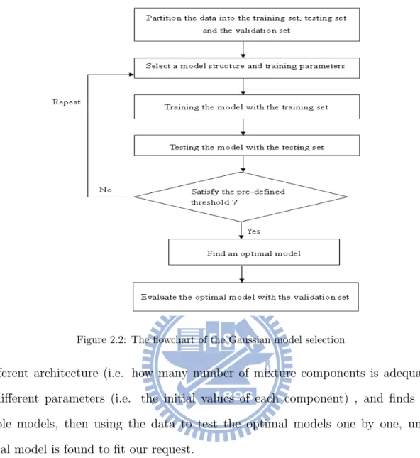
Model selection is the problem of choosing a proper model from a set of potential models by getting a tradeoff between the best inductive bias and the model complexity, that means attempt to select the proper parameters to create a model of optimal complexity from the given training data. For example, when we want to select the model of the neural network, one will separate the given data into three complementary subsets: the training set, the testing set and the validation set. The candidate models will train using the training set, and testing by the testing set, finally evaluate by the validation set. From the flowchart of the Gaussian model selection (see fig.2.2), we can see that it is very time consuming when selecting a optimal model from the given data. It must configure several candidate models
Figure 2.2: The flowchart of the Gaussian model selection
in different architecture (i.e. how many number of mixture components is adequately?), and different parameters (i.e. the initial values of each component) , and finds all the possible models, then using the data to test the optimal models one by one, until the optimal model is found to fit our request.
As a result, when selecting a model, the performance validation of a model has became a key point. In addition, there are many architectures of model can be selected, a number of different parameters of a model can be chosen, and lots of different training ways can be picked, which made the problem of model selection becomes more difficult. Consequently, we need a criterion to follow and let us to decide which model is optimal. However, to choose a proper criterion is still a difficult task in different applications. There are many methods to tackle the problem of model selection, for example, in empirical way like bootstrap [23], Cross-validation [24] and jackknife [25], and in theoretical way like Akaike information criterion (AIC) [26] and Bayesian information criterion (BIC) [27].
method which is one of the empirical way, because it allows the system to construct new data samples which are based on the original small data set, and then to estimate the stability of the parameters. Finally, we will apply the bootstrap method to decide the proper number of the components in the mixture of Gaussian, which was used for our feature in the CBIR system.
To determine the optimal number components in mixture Gaussian, we introduce the Bootstrap method for model selection which is still a difficult task. An modified version from the original bootstrap method which is called the Weighted Bootstrap (WB)[28] that can select the correct model better than the original method was proposed in Chapter 4. The experimental results show that the weighted bootstrap procedure can be applied to select the optimal number in Mixture Gaussian which can be using for approximating the histogram of the images as the feature in the CBIR system.
2.3
Content-Based Image Retrieval
Content-based image retrieval (CBIR) system has been build over the last few decades, and is a interesting problem due to abundant contents and information hiding in images. How to extract proper features is still an open issue for the image retrieval problem.
According to different query methods, image query systems can be divided into two categories: (1) the full automated query, and (2) the user assist query. For a full automated query, global features, such as color histograms, are often used for image retrieval. Some early developed systems, such as QBIC [29], Virage [30], Photobook [31], VisualSEEk and WebSEEk [32] basically applied global features for image retrieval. However, using global features for image indexing, a query system may ignore some significant local details of sample images, so as to retrieve some undesired images.
Instead of using global features of an image, the user assist query systems, such as the Netra [33] and Blobword [34], adopt local features to represent or to index an image. In these systems, the local features often obtained from some regions or subimages, which are manually segmented or sketched from an image first, and then various visual features of
these regions can be extracted. In general, the query and retrieving performance of these systems are usually better than the systems which is based on the global feature. However, their performance are heavily dependent on how to precisely segmenting or skillful sketching regions from an image.
From the above discussion, it can conclusion that features used to represent the contents of the image can be roughly divided into two types: (1) global features that extracted from a whole image, and (2) local features that extracted from local regions (subimages) of the image. Since the global features lack spatial information among the interested regions in the image, the retrieval results are not satisfactory. Hence, local features are adopted to represent the interested image more appropriate. Some of the systems, i.e., SaFe [35], uses the local features and spatial relationship among the interested subimages in the image as a new kind of features. The challenge of the local features extraction is how to automatically choose interested subimages from a sample image. Even for human, different interested subimages are selected from a single image due to their different point of views.
For the past decades, automatically segmenting an image into regions is still a diffi-cult task in image processing research [36, 37, 38]. Instead of emphasizing on the precise region segmentation, Integrated Region Matching (IRM) metric [1] proposed a robusted measurement of the similarity between regions, without requiring accurate region segmen-tation. Later, two region-based fuzzy feature matching approaches [7, 39] are proposed to characterize each region with a fuzzy feature set. As far as image retrieval, these methods demonstrate substantial improvement on the query accuracies, such as 46.8% [6], 47.7% [7], and 53.8% [39].
In order to narrow the gap between high-level concepts and low-level features, the user assist query systems also involve relevance feedback(RF) [40] information to improve the hit rate of the retrieval system. Originally, the mechanism of relevant information was applied to text retrieval( i.e. SMART system [41]). It really can improve the retrieval results. Later, T. S. Huang apply this technology to the image searching, and it is proved that relevance feedback (RF) is an important tool which can improve the performance of
CBIR( MARS [5]) . The early relevance feedback schemes focus on the heuristic formulation for empirical parameter adjustment [42, 43]. At a later time, researchers solve this problem by using the optimal learning algorithms [44], such as Bayesian learning algorithms [45], boosting techniques [46], discriminant-EM algorithm [47], Support Vector Machine, and other kernel-based learning machines. Until now, they are still the open issues that how to incorporate relevance feedback information and how to adjust the similarity measure to refine the query results.
Chapter 3
Multiple Instance Learning Methods
Since there are abundant contents hiding in an image, it can try to think about the image retrieval problem in a particular way, like a multiple-instance problem. According to the concept of the multiple-instance problem, a set of conceptual images called positive images and a set of non-conceptual images called negative images are given. In each image of the image database, several instances are extracted. Then, the system is trained to learn the conceptual image based on these instances extracted from the given images.
3.1
Introduction
Before training the system for indexing images, multiple feature vectors are extracted from the multiple instances of several exemplar training images. Then, the system are trained according to the proposed EM based Multiple-Instance learning algorithm[48]. Finally, the testing images are evaluated using Bayesian decision rule for indexing and classification.
In order to represent the rich content of an image without precisely image segmentation, the image retrieval problem can be considered as a multiple-instance learning problem, where each image is labelled either positive or negative. A positive image contains a set of instances (subimages) where not less than one instance is conceptual related to the user. On the other hand, a negative image contains instances where no one is conceptual related to the user. The multiple-instance learning problem was first appeared in[49]. Since a label is given to an image instead of each instance in the image, the labelling of an instance is
neither precisely nor completely. Therefore, the goal of the multiple-instance learning is to search the “concept area” which is at the location near to the intersection of the positive image features and far from the union of the negative image features in the feature space. Dietterich et al. proposed an algorithm [13] for learning axis-parallel concepts in the drug discovery problems, but their algorithm might only suitable for the feature distributions formed as axis-parallel rectangles. Later, O. Maron and A. Lakshmi Ratan [19] proposed the Quasi-Newton based framework to learn multiple-instance problems. In order to avoid the local maxima, they used every instance in positive images as initial points. Without a proper initial setting, the learning speed of the framework might be slow down .
However, segmenting and deciding the interested subimages from an image automat-ically and precisely are very difficult tasks. In order to extract preferred subimages of images without image segmentation, the image retrieval problem is reduced to the multiple-instance learning problem. The label which is given to an image by the user is ambiguously in multiple-instance based image retrieval problem. A positive bag contains a set of in-stances (subimages) if at leaset one instance in the bag belongs to the user’s favored image class. A negative bag contains a set of instances if all instances in the bag do not belong to the user’s favored image class. Since the labelling is given to the bag, not for individual instance, the information for an instance is not accurately or entirely, the conventional supervised learning framework is not suitable to learn these problems.
In order to avoid the influence of segmentation, and still can retrieve the enough char-acteristic and information to describe the image content, and capture relevance feedback mechanisms provided by the users effectively, then translate these information into the contributing to enhance the accuracy of the search engine, we try to regard the image searching problem as ”multiple-instance learning problem” [13, 19] , and to capture users relevance feedback mechanisms by the use of neural network learning mechanism, finally training the concept of the example images which the users is interesting.
3.2
The EM based Multiple-Instance Learning Method
When treating the image retrieval problem as the multiple-instance problem, each image will be labelled by the subjective concept of the user with a set of positive example images and a set of negative example images. A user can express their desired concepts through the interface provided by the system, and the concepts which the user want to describe may be a certain objects or just an abstract concepts. For example, when the users want to identify an images with ’waterfall’, then the region of the ’waterfall’ or the subimage of the ’waterfall’ in that image is one instance. User can describe her/his concepts by labelling the image as a positive example if it contains at least one instance of the ’waterfall’, or a negative example if it does not contain any instance of the ’waterfall’.
The above definition accords with the characteristic in CBIR system when the user would like to submit their images. For example, when the user submits the images which she/he is interested, using several images to describe their concepts in the way of Query-by-Example. Why these examples will be submitted to the system? It is because these example images contain certain region or several regions meet the user’s concept.
The label of the image which is given by the user is based on the whole image to the content, rather than individual examples of images, so the system does not know each instance in a image belongs to which class, that is to say, the issue of the CBIR accords with the characteristic of the instance learning problems. The goal of multiple-instance learning is to find a concept that correctly classifies the labels on the training set and to predict the labels for new images.
3.2.1 The Energy Function of the EM based Multiple-Instance Learning Method In the Multiple-Instance learning, conceptual related (positive) images and conceptual unrelated (negative) images are designed for reinforced and antireinforced learning of a user’s interesting image class. Each positive training image contains at least one interested subimage related to the desired image class, and each negative training image should not contain any subimage related to the desired image class. The target of the
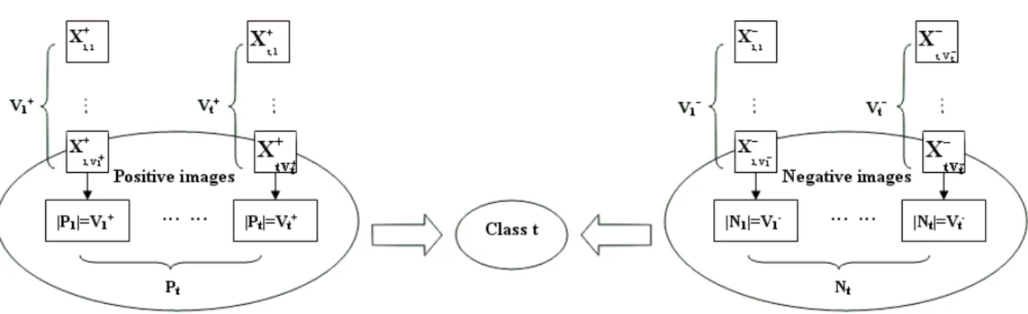
Multiple-Figure 3.1: The schematic of the positive and negative for the class t
Instance learning is to search the optimal point of the image class in the feature space, where the optimal point is close to the intersection of the feature vectors extracted from the subimages of the positive training images and is far from the union of the feature vectors extracted from the subimages of the negative training images.
For example, if one wants to train an image class t with Ptpositive images and Nt
neg-ative images. Each positive image has V+
t instances (i.e. |P1| = V1+, |P2| = V2+, · · · , |Pt| =
V+
t ), and each negative image has Vt− instances (i.e. |N1| = V1−, |N2| = V2−, · · · , |Nt| =
V−
t ). It can denote the kthfeature vector extracted from the kthinstances of the ithpositive
image as X+
ik, and the kthfeature vector extracted from the kthinstances of the ith negative
example as X−ik. The schematic of the positive and negative for the class t is shown as Figure 3.1.
The probability that X+
ik belongs to class t is P (t | X+ik), and the probability that X−ik
belongs to class t is P (t | X−
ik). A measurement called Diverse Density is used to evaluate
that how many different positive images have feature vectors near a point t, and how far the negative feature vectors are from a point t. The Diverse Density for a class t is defined as [18] DDt = Pt Y i=1 (1 − Vt+ Y k=1 (1 − P (t | X+ ik))) Nt Y i=1 ( Vt− Y k=1 (1 − P (t | X− ik))). (3.1)
3.2.2 The computation of Diverse Density
The optimal point of the class t is appeared where the Diverse Density is maximized. By taking the first partial derivatives of Eq.(3.1) with respect to parameters of the class t and setting the partial derivatives to zero, the optimal point of the class t can be obtained. Suppose the density function of the class t is a D-dimensional Gaussian mixture with uncorrelated features. The parameters are the mean µtcd, the variance σtcd2 , and the cluster
prior probability ptc of each dimension d in each cluster c of the class t. The estimating
parameters of the class t can be derived by ∂
∂µtcdDDt= 0, ∂ ∂σ2 tcdDDt= 0, and ∂ ∂ptcDDt = 0. Thus µtcd = Pt X i=1 ( Pti 1 − Pti ) V+ t X k=1 Qtc(X+ik)x+ikd − Nt X i=1 V− t X k=1 Qtc(X−ik)x−ikd , Pt X i=1 ( Pti 1 − Pti ) V+ t X k=1 Qtc(X+ik) − Nt X i=1 V− t X k=1 Qtc(X−ik) , (3.2) σ2 tcd = XPt i=1 ( Pti 1 − Pti ) Vt+ X k=1 Qtc(X+ik)kx+ikd− µtcdk2 − XNt i=1 Vt− X k=1 Qtc(X−ik)kx−ikd− µtcdk2 , XPt i=1 ( Pti 1 − Pti ) Vt+ X k=1 Qtc(X+ik) − XNt i=1 Vt− X k=1 Qtc(X−ik) , (3.3) ptc = XPt i=1 ( Pti 1 − Pti ) Vt+ X k=1 Qtc(X+ik) − XNt i=1 Vt− X k=1 Qtc(X−ik) , XPt i=1 ( Pti 1 − Pti ) Vt+ X k=1 ( P (t|X + ik) 1 − P (t|X+ik)) − XNt i=1 Vt− X k=1 ( P (t|X − ik) 1 − P (t|X−ik)) , (3.4) where P (c|X? ik, t) = ptc· P (X?ik|c, t) P (t|X? ik) , (3.5) P (t|X? ik)(l) = P (X? ik(l)|t)Pt P (X? ik) , (3.6) Pti = Pi Y k=1 (1 − P (t|X? ik)) ,
Qtc(X?ik) = P (t|X? ik)P (c|X?ik, t) 1 − P (t|X? ik) , P (X?ik|c, t) = QD 1 d=1(2πσ2tcd) 1 2 · exp(−1 2 D X d=1 (x ? ikd− µtcd σtcd )2),
and the l represents the iterative number of the EM algorithm which is introduced below, and the notation ? represents + or −.
According to Eqs.(3.2), (3.3), and (3.4), an EM based Multiple-Instance learning al-gorithm to learn these parameters was proposed.[48]. The EM based Multiple-Instance learning algorithm contains two steps: the expectation step (E-step) and the maximiza-tion step (M-step). The algorithm is described as follows.
EM based Multiple-Instance learning algorithm
1. Choose an initial point in the feature space, and let its parameters are µ(0)tcd, σ2(0)tcd , and
p(0)tc .
2. E-Step : Using the calculated model parameters µ(l)tcd, σtcd2(l), p(l)tc, Eqs.(3.5) and (3.6), estimate P(l)(c|X?
ik, t) and P(l)(t|X?ik).
M-Step : Using the estimated P(l)(c|X?
ik, t) and P(l)(t|X?ik), compute the new model
parameters µ(l+1)tcd , σtcd2(l+1), and p(l+1)tc according to Eqs.(3.2), (3.3), and (3.4). 3. Calculate the diverse density DD(l+1). If (DD(l+1)−DD(l)) is smaller than a predefined
threshold ², then stop the process. Otherwise, incremental iterative number l and loop step 2.
As we can see, the proposed algorithm provides comprehensive procedures to maxi-mizing the measurement of diverse density of the given multiple instances X+ik and X−ik. Furthermore, the new EM based learning framework converts multiple-instance problem into a single-instance treatment by using EM algorithm to estimate and to maximize the instance responsibility for the corresponding label of each bag of instances.
Gaussian model of each class, that is, a problem about the model selection, is still an important issue which we want to tackle in the next section.
Besides, in order to build a more powerful model, we consider the relationship between weight and features, for example, when the user click certain point to show the concept of the image, the importance of the neighbor pixels of that point should be decreased gradually when the distance of the neighbor points more far away from the that point, will also be included in the future systems.
In the next section, we combine the proposed EM based Multiple-Instance Learning Method with the probabilistic variant of the decision-based modular neural networks(PDBNN)[50] to become a new learning model : Multiple-Instance Neural Network (MINN). The new learning model let the user’s concept forms in the training phase and gets the relevance feedback from the users in the testing phase. At the same time, we propose a new method of the instance extraction from the image, which can consider the the weighting of the feature.
3.3
The Multiple-Instance Neural Network
The Multiple-Instance Neural Networks (MINN) is a probabilistic variant of the decision-based modular neural networks [50] for classification. One subnet of the MINN is designed to represent one class of a multiple-instance problem. Based on the given positive example images and negative example images of a concept from the user, the MINN performs the parameters updating process to the subsets to formulate the concept. The updating rule contains reinforced learning to the subset corresponding to the positive images and anti-reinforced learning to the subset corresponding to the negative images.
3.3.1 The Discriminate Functions of MINN
Given an image I and a set of i.i.d. patterns X = {x(t); t = 1, 2, · · · , N } , where each element is a feature vector x(t) extracted from each instance in the image I. It can assume that a concept class ωi for the density as a linear combination of component densities
p(x(t)|ωi, Θri) in the form p(x(t)|ωi) = Ri X ri=1 Prip(x(t)|ωi, Θri), (3.7)
where Pri is the prior probability of a cluster ri, and Θri represents the parameter set
{µri, Σri}. By definition,
PRi
ri=1Pri = 1, where Ri is the number of clusters in ωi.
The discriminate function of the MINN models is defined as:
φ(X, Ωi, k) = ln(− ln( k Y n=1 Dn)) = ln(− k X n=1 ln Dn), (3.8)
where {Dn; n = 1, 2, · · · , N } is a decreasing series obtained by sorting the {p(x(t)|ωi); t =
1, 2, · · · , N }, and Ωi = {µri, Σri, Pri, Ti}. Ti is the output threshold of the subnet i. The
parameter k is a user determined parameter called bounded number, which is the number of instances to be related to the class ωi. If k is set to one, only the nearest instance of the
concept class ωi is considered. If k is equal to the total number of instance in the given
image, all instances in the given image are considered. The smaller value of φ(X, Ωi, k)
means the given image I is more similar to the class ωi.
In most general formulation, the density function p(x(t)|ωi, Θri) in (3.7) should be
proximated by the distribution with full-rank covariance matrix. However, for those ap-plication that deal with high-dimension data but a finite number of training patterns, the training performance and storage space discourage such matrix modelling. A natural sim-plifying assumption is to assume uncorrelated features of unequal importance. That is, suppose that p(x(t)|ωi, Θri) is a D-dimensional distribution with uncorrelated features and
in order to make sure that the negative log likelihood in Eq.(3.8) is positive, the component density function is defined as
p(x(t)|ωi, Θri) = exp · −1 2 ¡ (x(t) − µri) TΣ−1 ri (x(t) − µri) ¢¸ (3.9) where x(t) = [x1(t), x2(t), · · · , xD(t)]T is the input pattern, µri = [µri1, µri2, · · · , µriD]
T,
and diagonal matrix Σri = diag[σ2ri1, σ
2
ri2, · · · , σ
2
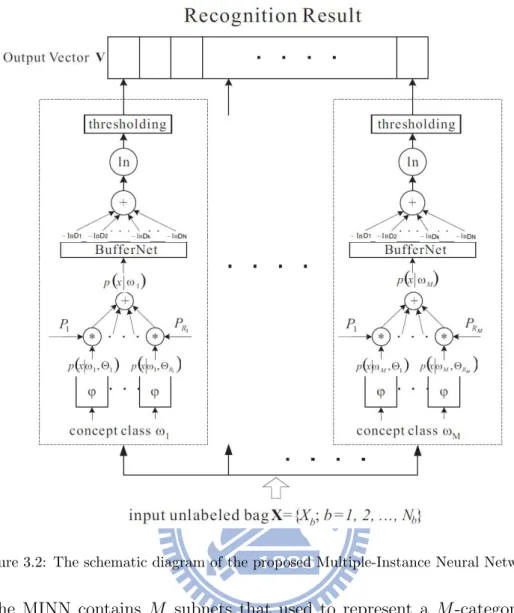
Figure 3.2: The schematic diagram of the proposed Multiple-Instance Neural Network
Fig. 3.2, the MINN contains M subnets that used to represent a M-category multiple-instance learning problem. Inside each subnet, an elliptic basis function (EBF) is used to serve as the basis function for each cluster ri
ϕ(x(t), ωi, Θri) = − 1 2 D X d=1 (xd(t) − µrid) 2 σ2 rid . (3.10)
After passing an exponential activation function, exp{ϕ(x(t), ωi, Θri)} can be viewed as a
distribution described in Eq.(3.9).
3.3.2 The Energy Function of MINN
In multiple-instance learning problems, the best matched class fells within a region which is near to the intersection of the positive images, and far away from the negative images. In other words, the best matched class fells within the area which contains most instances
of positive images and very few instances of negative images.
For each class ωi, given a set of images Xi = {Xib; b = 1, 2, · · · , M }, where Xib is a set
of instances {xib(t); t = 1, 2, · · · , Nb} in a image b. The energy function of the class ωi is
defined as E(Xi, Ωi) = ln(− ln( M Y b=1 Nb Y t=1 p(xib(t)|ωi)) = ln(− M X b=1 Nb X t=1 ln p(xib(t)|ωi)). (3.11)
If there is only one image in the Xi, the energy function is reduce to (3.8), where the
bounded number k of Eq.(3.8) is set to the number of instances in the image.
In order to rigorously test how the MINN and the proposed energy function (3.11) deal with multiple-instance learning problems, we generated the following data set. There are two classes in the data set. In each class, ten bags are generated, each with 100 instances. The concepts of the class 1 and class 2 are the Gaussian distributions with the same variance 0.04. The mean of class 1 is (0.2, 0.8), and the mean of the class 2 is (0.8, 0.2) in the feature space. In each class, five bags are labeled positive and the rest are labeled negative. In each positive bag, 20 instances are generated randomly from the distribution of the concept class and 80 instances were generated uniformly at random. In each negative bag, 100 instances were generated uniformly at random, but none of the instances fell within the designated concept class. The distribution of the instances from each bag is shown in Figure 3.3. The instances from the positive and negative bags are denoted as ‘+’ and ‘x’ respectively. The trajectory of the predicted positions of the class concepts during the training phase of the MINN are shown in Fig.3.3.
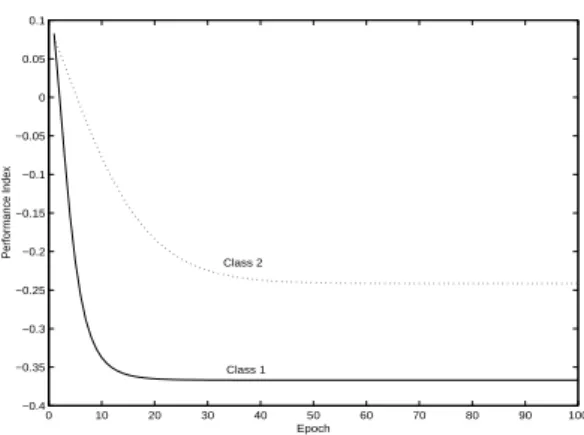
The change of the energy during the training phase are shown in Fig.3.4. It is clear that the energy function decreased after each iteration in the training phase of the MINN.
0 0.1 0.2 0.3 0.4 0.5 0.6 0.7 0.8 0.9 1 0 0.1 0.2 0.3 0.4 0.5 0.6 0.7 0.8 0.9 1 (a) 0 0.1 0.2 0.3 0.4 0.5 0.6 0.7 0.8 0.9 1 0 0.1 0.2 0.3 0.4 0.5 0.6 0.7 0.8 0.9 1 (b)
Figure 3.3: The artificial data set (a) Class 1, and (b) Class 2. The instances from the positive and negative bags are denoted as ‘+’ and ‘x’ respectively. The trajectory of the predicted points of the class concepts during the training phase are denoted as ‘.’.
0 10 20 30 40 50 60 70 80 90 100 −0.4 −0.35 −0.3 −0.25 −0.2 −0.15 −0.1 −0.05 0 0.05 0.1 Epoch Performance Index Class 2 Class 1
Figure 3.4: The class energy decreased monotonically during the training phase of the MINN, where the bold line implies the class 1 and the dotted line implies the class 2.
3.3.3 The Training Phase
It can see that minimizing E(Xi, Ωi) with respect to Ωi, the class ωi will be located where
there are most instances of the images. On the other hand, maximizing E(Xi, Ωi) with
respect to Ωi, the class ωi will be located where there are very fewer instances of the
images.
After given a set of positive training images X+i and a set of negative training images X−
i of the corresponding class, the following reinforced and anti-reinforced learning rules
are applied to the corresponding subset. Reinforced Learning:
Ω(m+1)i = Ω(m)i − η∇E(X+
i , Ωi), (3.12)
Antireinforced Learning:
Ω(m+1)i = Ω(m)i + η∇E(X−i , Ωi). (3.13)
In (3.12) and (3.13), η is a user defined learning rate 0 < η ≤ 1, we set η = 0.5 in this dissertation. ∇E are gradient vectors, which are computed as follows:
∂E ∂µrid = 1 ln f (Xi) M X b=1 Nb X t=1 p(Θri|ωi, xib(t)) (xibd(t) − µrid) σ2 rid , (3.14) ∂E ∂σ2 rid = 1 2 ln f (Xi) M X b=1 Nb X t=1 p(Θri|ωi, xib(t)) (xibd(t) − µrid)2 σ4 rid , (3.15) where f (Xi) = PM b=1 PNb t=1p(xib(t)|ωi) and p(Θri|ωi, xib(t)) = p(xib(t)|ωi, Θri) p(xib(t)|ωi) (3.16) is a posterior probability of the cluster ri in concept class ωi given xib(t)
As to the conditional prior probability Pri, since the EM algorithm can automatically
satisfy the probabilistic constraints PRi
ri=1Pri = 1 and Pri ≥ 0, it is applied to update the
Pri as follows: Prnewi = 1 M · Nb M X b=1 Nb X t=1 p(Θri|ωi, xib(t)). (3.17)
Threshold Updating: The threshold value of MINN can also be learned by the reinforced and anti-reinforced learning rules. For example, given a class ωi, if a positive image of
ωi is misclassified, the threshold Ti needs to be increased because the Ti is too small
to reject this positive image. On the other hand, if a negative image is misclassified, the Ti should be reduced since the Ti is too large to accept this negative image. An
adaptive learning rule to train the threshold Ti is proposed as follows:
Ti(m+1) = Ti(m)+ γ∆Ti(m), (3.18)
where γ is a user defined learning rate 0 < γ ≤ 1, and the value of γ can set to
γ = 0.5. ∆Ti(m) is defined as Ep(m)− En(m), where Ep(m) is the misclassified rate of the
positive images in the mth iteration, and E(m)
n is the misclassified rate of the negative
images in the mth iteration.
3.3.4 The Testing Phase
As shown in Fig.3.2, an unlabel image is input to the MINN, then the MINN labels the given image with one or several matched classes. First, an unlabel image is applied to all subnets in the MINN. In each subnet, computation is performed according to the discriminate function (Eq.3.8). Then the results of discriminate function are compared with the threshold Ti. Finally, the ith element of the retrieval result vector V is set to 1
if the value of the discriminate function is smaller than Ti, which implies that the given
image belongs to the concept class i. Otherwise, the ith element of the recognition result
vector V is set to 0 if the value of the discriminate function is larger than Ti, which implies
that the given image does not belong to the concept class i. From the output vector, one can recall which concept classes the given image belongs to.
3.3.5 Image Indexing with Histogram Approximation
Suppose images are digitized as 24 bits RGB, meaning that 8 bits or 256 linear levels of brightness for red, green, and blue components. For the sake of the more perceptive to the human vision, we calculating the histograms of each components in the Lab color space,
then three histograms corresponding to the three color components L, a, b of the masked image are combined as a histogram vector H = [h1, h2, · · · , h256∗3−1]T. The nth element in
H is evaluated as
H(n) = Σx,yGm(x, y), {(x, y); Ic(x, y) = n mod 256}, (3.19)
where Gm(x, y) is the Gaussian-like mask image which will be defined in (5.2), Ic(x, y)
is the intensity value of the cth color channel at the position (x, y) in the masked image
Gm(x, y), and c is the quotient of the n divided by 256.
Instead of using color histograms as features of images, the proposed system used the parameters of mixture density functions which approximate color histograms of each image as features so as to decrease the dimensions of features and speed up the response time of querying. In information theory, the cross entropy[51] between two probability distri-butions measures the average number of bits needed to identify an event from a set of possibilities, and the cross entropy for two distributions over the same probability space can be used to measure the similarity for two distributions.
Define p(t|Θr) is a one-dimensional Gaussian distribution, and Θr represents the
pa-rameter set {µr, σ2r} for a cluster r, where µr and σr2 are the mean and the variance of a
cluster r, respectively. Then
p(t|Θr) = 1 √ 2πσr exp µ −1 2 (t − µr)2 σ2 r ¶ , (3.20)
Let p(t|Θr) to be one of the Gaussian distributions that comprise P (t), and Pr denotes
the prior probability of the cluster r. Then P (t) is a mixture Gaussian distribution, which can express as below:
P (t) =
R
X
r=1
Prp(t|Θr), (3.21)
where R is the number of clusters in P (t). By definitionPRr=1Pr = 1. We can take the
value of the Pr = 1/R, and set σr2 = 0.05.
Since a color histogram of an image can be regarded as an one-dimensional vector, given a color histogram H(n), where 0 ≤ n ≤ N, and a mixture of Gaussian distributions P (t),
the similarity between H(n) and P (t) is measured by using their cross-entropy − N X n=0 H(n) ln P (n). (3.22) It is well known that cross-entropy minimization is frequently used in optimization, in Eq.(3.22), the cross-entropy has the minimum value when P (n) is equalized to H(n), where
n = 0, 1, · · · N. Hence, the EM algorithm is applied to adjust the parameters Θr and Pr
of each cluster r in P (t) to minimize Eq.(3.22) so as to approximate H(n). The updating equations for the parameters in the cluster r of mixture model P (t) are
µnewr = PN n=0H(n)pold(Θr|n)n PN n=0H(n)pold(Θr|n) , (3.23) (σnew r )2 = PN n=0PH(n)pold(Θr|n)(n − µnewr )2 N n=0H(n)pold(Θr|n) , (3.24) Pnew r = PN n=0H(n)pold(Θr|n) PN n=0H(n) , (3.25)
where p(Θr|n) is a posterior probability of the cluster r given n, which is defined as
p(Θr|n) = PRp(n|Θr) r=1Prp(n|Θr)
. (3.26)
In each EM iteration, there are two steps: Expectation (E) step and Maximization (M) step. The M step maximizes a likelihood function which is further refined in each iteration by the E step. In each iteration, we first compute the posterior probabilities of the clusters using Eq.(3.26) in E-step, and calculate the new parameters of the model using Eqs.(3.23),(3.24) and (3.25) in M-step.
Chapter 4
Bootstrap for Model Selection
For a model selection problem, for example, choose a MLP model is equivalent to the selection of its network architecture, such as the number of hidden layers, hidden nodes, etc. If we want to select an optimal model from several candidate models, one possible approach is to test all the possible models exhaustively with the data set can obtained for the specific problems. But such an exhaustive approach is very time-consuming and not practical. In general, we can separate the given data into three subsets: the training set, the testing set and the validation set. First, training these candidate models using the training set, then testing by the testing set, finally evaluate by the validation set. This is the so called hold-out method. The cross-validation method is one of the approach of the hold-out method.
The k-fold cross validation is a common types of cross-validation method. First, data is divided into k classes, each time holding a class as the test data, while the remaining k − 1 class is used for training models, then repeated k times, finally calculated the average error rate to find the optimum model. If the amount of K data is set to N, that is, a certain single data is keep as the test data, while the remaining N − 1 data is used to training the model, then repeated N times, this is the so called leave-one-out cross validation. In fact, the quality of error estimates is closely related to how to partition the data into training set and testing set. If the cut point of the data is inadequate, it will seriously affect the results of evaluation. How to reduce the effect of how the the data is partitioned is an
important issue. One way is to separated data into training set and testing set randomly, then the so called cycle of the split-training-testing will repeated in order to reduce the uncertainty and the bias caused by how the data is partitioned.
More importantly, the sample data obtained is usually very limited. When data is limited, it’s very difficult to separate the data into the training group and test group ideally. The method of bootstrap is one of the re-sampling method, which can construct a series of new sample sets from the original data, to measure the stability of the parameters which is estimated for a model.
The bootstrap method is similar to the method of the leave-one-out cross validation, the difference is that the former does not always remain one data as the test data, but treats the entire data as a test set, and each time drawn N data from the original data set with replacement randomly, then repeat several times(i.e. B times). Finally, these B data sets can treat as B training sets, which is similar to the K of the K-fold cross-validation to estimate the best model.
Therefore, we use the Bootstrap method applied to the issue of model selection to reduce the cost of computation in the process of data simulation. While improving the original bootstrap method which is proposed by Kallel et al. [52] (Original Bootstrap, referred to as: OB) to assess the stability of model parameters, as a criterion for model selection, then propose a method of treating the absolute value of the residual error as weights (Weighted Bootstrap, referred to as: WB). The experimental results show that weighted bootstrap algorithm can be applied to select the optimal number of the mixture Gaussian, and it’s performance is better than the original bootstrap method.
4.1
Bootstrap Introduction
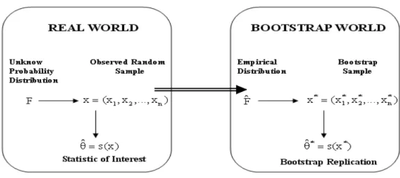
The bootstrap method is also called resampling computations techniques, was originally proposed by Efron, B. [53] in 1979 for use in setting independent and identically dis-tributed (i.i.d.) random variables. Consider a sample data drawn from distribution func-tion F = fx(X; θ), X = (x1, x2, · · · , xn). Using the statistics ˆθ = s(X) of X to estimate the
Figure 4.1: The schematic diagram of the bootstrap
true parameters θ. Because the parameter θ of the distribution function F = fx(X; θ) is
unknown, in order to make the estimation more accurate in the situation of small sample, we can draw from the original sample X the same size n randomly with replacement B times. These B sample data sets is called bootstrap samples(see figure 4.1 [23]), and the probability of each sample be drawn is PU = (x∗bi = xj) =
1
n, i, j = (1, 2, · · · , n) , that
means the probability of each sample x1, x2, · · · , xn be drawn is uniform. The new sample
data sets after resampling can be labelled X∗b = (x∗b
1 , x∗b2 , · · · , x∗bn), b = 1, · · · , B. The
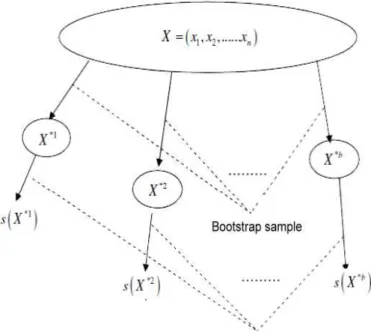
process of the resampling of the bootstrap is shown in figure 4.2 [23].
According the empirical distribution ˆF , it construct bootstrap replicates X∗b and can
get B estimates ˆθ∗b = s(X∗b) by above resampling process. Take the mean of the sample
data as a example, the mean of the original sample X is s(X) = 1
n
n
X
i=1
xi, and the mean
of the bootstrap sample X∗b can be written as s(X∗b) = 1
n
n
X
i=1
x∗bi . Consequently, we can compute the B standard derivations ˆσboot(ˆθ) of the estimates ˆθ :
ˆ σboot(ˆθ∗) = h 1 B − 1 B X b=1 (ˆθ∗b− ˆθ∗(.))2i1/2 where ˆ θ∗(.) = 1 B B X b=1 ˆ θ∗b
Figure 4.2: The schematic diagram of the bootstrap resampling
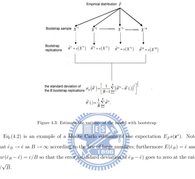
The figure 4.3 is the process of estimating the standard derivation by the bootstrap. By using the empirical distribution function ˆF , it can be replaced the true unknown
dis-tribution function F . Besides, by applying bootstrap resampling, one can construct the hypothesis testing and the confidence interval in the statistical.
The ideal bootstrap estimate of the expectation of s(z) is ˆ
e = EFˆs(z∗), (4.1)
where ˆF is the empirical distribution function, EFˆ is the expectation under ˆF , and z∗ =
{z∗
1, . . . , zn∗} is drawn randomly from z with replacement. Unless s(z) is the mean or some
other simple statistic, it is not easy to compute ˆe exactly, so it can approximate the ideal bootstrap estimate by ˆ eB= 1 B B X b=1 s(z∗b), (4.2)
where each z∗b is a sample of size n drawn with a replacement from z, B is the number
Figure 4.3: Estimate the variance of the model with bootstrap
Eq.(4.2) is an example of a Monte Carlo estimate of the expectation EFˆs(z∗). Note
that ˆeB → ˆe as B → ∞ according to the law of large numbers; furthermore E(ˆeB) = ˆe and
var(ˆeB− ˆe) = c/B so that the error (standard deviation of ˆeB− ˆe) goes to zero at the rate
1/√B.
4.2
Weighted Bootstrap for Gaussian Model Selection
Let B0 be a data set of size n, that is, n = card{B0},
B0 = {(x1; y1), · · · , (xn; yn)},
where xi is the ith value of a p-vector of explanatory variables and yi is the response to xi.
First, we use the data set B0 to estimate the parameter θ of the model and the resulting
least-squares estimator of θ is denoted by ˆθ. Thus, the residual for the ith observation is
denoted by ei and is defined as follows:
Frequently, in applications, the data set contains some cases that are extreme. These extreme values could be noise or caused by some uncertainty; that is, the observations for these extreme cases should be well separated from the remainder of the data, because these extreme cases may involve large residuals and often have dramatic effects on the fitted model. It is therefore important to study the extreme cases carefully and their influence should be reduced in the fitting process. However, in uniform resampling, that is, random resampling with replacement from B0, each sample value is drawn with the same
probability 1/n. This resampling technique discards the influence of these extreme cases. An alternative to discarding extreme cases that is less severe is to damp the influence of these cases. This is the purpose of our proposed weighted bootstrap approach.
Under weighted bootstrap (sampling is conducted with replacement), each data point (xi; yi) is assigned a probability qi of being selected on any given draw, where
P
qi = 1.
Taking qi = 1/n for each i, we obtain the original bootstrap method. To determine what
qi’s should be used, we intuitively want to reduce the influence of extreme cases so that the
qi varies inversely with the size of absolute value |ei|. It is well known that an exponential
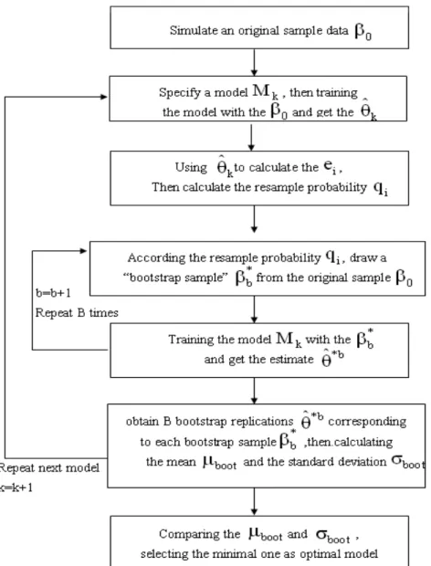
operation is highly useful in dealing with a similarity relation by Zadeh [54] and Shannon’s entropy process [51]. We therefore choose
qi ∝ exp(−|ei|). That is, qi = exp(−|ei|) Pn j=1exp(−|ej|) , i = 1, · · · , n.
Based on the above discussion, we give the weighted bootstrap algorithms as follows: Algorithm : Weighted Bootstrap Algorithm
S1 . Simulate an original sample data B0 = {(xi; yi)|i = 1, · · · , n}.
S2 . Specify a candidate model Mk, k = 1. Training the model Mk with the B0 and get
the ˆθk.
probability distribution {qi|i = 1, · · · , n} to be qi = exp(−|ei|) Pn j=1exp(−|ej|) , i = 1, · · · , n.
S4 . With the original sample B0 fixed, draw a “bootstrap sample” of size n called
B†= {(x†
i; y†i)|i = 1, · · · , n}, under resampling probability distribution qi from S3.
S5 . For this bootstrap sample B†, estimates θ by minimizing Pn i=1
³
yi†− y(x†i; θ) ´2
, we get ˆθ†. Then we have the mean of the squares of the residuals on the test base B
0: T MSE = 1 n n X i=1 ³ y†i − y(x†i; ˆθ†) ´2 .
S6 . Repeat S4 B times, we obtain B bootstrap replications corresponding to each bootstrap sample:
T MSE(1), · · · , T M SE(B).
and get the mean value and the standard deviation of the B bootstrap replications:
µboot = 1 B B X b=1 T MSE(b), σboot = ³ 1 B − 1 B X b=1 (T MSE(b) − µboot)2 ´1/2 .
S7 . Let k = k + 1 and repeat S2 for the next candidate model Mk+1.
S8 . Comparing the µboot and σboot for each model, selecting the minimal one as the
optimal model.
The flowchart of the Weighted Bootstrap Algorithm see Fig 4.4. According to Eq.(4.2), we have
µboot = 1 B B X b=1 T MSE(b) → 1 n n X i=1 e2i (say MSE), as B → ∞.
Usually, MSE is an estimate of σ2 and, by using the law of large number, we have
MSE = 1 n n X i=1 e2 i → σ2, as n → ∞.
It is natural to pose the question: “How accurate is MSE?”. σboot is the bootstrap
that a good model should have the small µboot and σboot. Therefore, to choose between
several models M1, M2, · · ·, the best one will be the one that has the best compromise to
simultaneously minimize µboot and σboot.
4.3
Experiment result : The Mixture Gaussian Selection
In the subsection 3.3.5 , we have introduced that a mixture Gaussian distribution P (t) for the density can be expressed as a linear combination of component densities p(t|Θr) in the
form P (t) = R X r=1 Prpr(t|Θr), (4.4)
and a histogram vector H(t) can be approximated to the P (t) using their cross-entropy with the EM algorithm which proposed in the subsection 3.3.5.
In the general case, before using the EM algorithm to estimate the mixture Gaussian, one must first decide the number of the component in a mixture Gaussian. However, how to determine the number of components is still an important issue. In this section, we using the form of the Eq.(4.4) to construct a mixture Gaussian which R = 3 as belows:
P3(t) = 1 3N( 1 3, 0.25) + 1 3N( 2 3, 0.25) + 1 3N(1.0, 0.25).(true model), (4.5) We generate a data set, say B0, with the sample size n = 300 based on the true model
Eq.(4.5)
B0 = (y1, · · · , yn), n = 300.
Based on the original data set B0, we consider the fitted model:
Mm(t) = m
X
r=1
Prpr(t|Θr), (4.6)
We also use the EM algorithm to estimate the parameters Θ = ( bP1, · · · , bPm, bΘ1, · · · , bΘm)
in Mm(t), say bΘ and generate a data set B1 = ( by1, · · · , byn), n = 300 from cMm(t) =
Pm
![Figure 2.1: An ambiguity spectrum [3]](https://thumb-ap.123doks.com/thumbv2/9libinfo/8399620.179153/18.892.126.750.134.239/figure-an-ambiguity-spectrum.webp)