多媒體資料完整性的快速認證

國

立

交

通

大

學

資訊科學系

碩

士

論

文

多媒體資料完整性的快速認證

Fast Approximate Message Authentication Codes for

Multimedia Data

研 究 生：林輝讓

指導教授：曾文貴 教授

ii

多媒體資料完整性的快速認證

Fast Approximate Message Authentication Codes for Multimedia Data

研 究 生：林輝讓

指導教授：曾文貴

國 立 交 通 大 學

資 訊 科 學 系

碩 士 論 文

A Thesis

Submitted to Institute of Computer Science and Engineering

College of Electrical Engineering and Computer Science

National Chiao Tung University

in partial Fulfillment of the Requirements

for the Degree of

Master

in

Computer and Information Science

August 2012

Hsinchu, Taiwan, Republic of China

iii

多媒體資料完整性的快速認證

學生：林輝讓 指導教授

曾文貴

國立交通大學資訊科學與工程研究所碩士班

摘

要

傳統的訊息認證方法是設計成能夠偵測任何訊息的更動，只要訊息有任何

不一樣就不會通過驗證者的認證。不同於傳統的訊息認證，Approximate

Message Authentication Codes (AMACs)是設計成能夠容忍合理範圍的錯

誤，訊息在錯誤不多的情形下也能夠通過認證，這在特性多媒體資料的認

證上十分有幫助，因為多媒體資料通常具有容忍錯誤的特性，少許的錯誤

並不會對資料的整體性造成太大影響而可以被驗證者接受。之前的 AMAC 研

究缺少調整認證彈性的機制，也缺乏對於不同 AMAC 之間的比較方法。我們

提出一快速且能夠調整容錯能力的 AMAC，並且透過實驗來驗證及比較我們

所提出的 AMAC 在不同錯誤容忍範圍下能夠正確分辨訊息錯誤比例的程度。

iv

Fast Approximate Message Authentication Codes for Multimedia Data

student：

Advisors：Dr.

Institute of

National Chiao Tung University

ABSTRACT

Different from conventional hard message authentication schemes that are designed to detect the slightest changes in messages, Approximate Message Authentication Codes (AMACs) are designed to tolerate a reasonable amount of differences in messages as multi-media data. Previous works on AMAC lack ability to adjust the authentication sensitivity and experiments on distinguishing messages. We formulate the robustness of AMACs as a hy-pothesis testing problem and apply random sampling to reduce the computation of AMACs. We then examine the robustness with experiments.

v

誌謝

首先要感謝指導教授曾文貴老師，感謝老師帶領我踏進入資訊安全這塊

領域，並教導我各種不同的知識及技術，讓我獲益匪淺。老師不只在學問

上教導我，對於學習的嚴謹以及做事的態度都是我處事的典範。老師對於

上台報告的指導相信也能夠在將來發揮很大的用處，讓我不太擅長的組織

及表達能力獲得練習及成長的機會。老師對於論文及研究耐心的指導也是

讓我能順利完成論文的主要因素。另外亦得感謝實驗室的學長姊的協助，

因為他們的熱心幫忙讓我克服許多學業上的問題。也感謝實驗室裡共患難

的同學們，一起準備學業的革命情感，互相幫助，才讓我能充足愉快地度

過這兩年的時光。

最後，謹以此文獻給我摯愛的雙親。

i

Content

中文摘要

Abstract

誌謝

Content

List of figures

Chapter 1 Introduction

Chapter 2 Related work

Chapter 3 Definitions

3.1 Statement of Problem ... 11

3.2 The Error model of tag ... 15

3.3 The error model of messages ... 15

3.4 Definitions of AMACs ... 16

3.5 Mutually independent AMACs ... 19

3.6 Probabilistic properties of mutually independent AMACs ... 20

Chapter 4 Our AMAC Algorithm

4.1 Initialization ... 23

4.2 Feature extraction ... 23

4.3 Random sampling ... 24

4.4 Masking... 25

4.5 Feature extraction: Tag function ... 26

4.6 Feature reduction: Quantization ... 27

ii

4.7 Verification ... 30

Chapter 5 Experiment

5.1 Experiment environment ... 32

5.2 Comparison of two different AMACs ... 33

5.3 Error estimation with tags ... 36

5.4 The effect of different sample rate ... 38

5.5 Accuracy comparison of different tag function ... 40

5.6 Effect of different thresholds ... 42

5.7 Effect of quantization ... 43

5.8 Accuracy under different condition ... 45

5.9 Comparison of computation time ... 47

Chapter 6 Security analysis and discussion

Chapter 7 Conclusion

iii

List of figures

Figure 1. Flow chart of a general multimedia authentication system ... 13

Figure 2. δm with different number of errors. ... 20

Figure 3. The flow chart of our AMAC scheme ... 22

Figure 6. False alarm versus true positive for different quantization ... 28

Figure 7. Different symbol size with fixed tag length ... 29

Figure 8. The scheme of AMAC verification ... 30

Figure 9. The probability that one AMAC symbol changes under different error ratio ... 34

Figure 10.δm with different number of errors and threshold. ... 36

Figure 11.δm with different number of errors and different thresholds ... 37

Figure 12. The effect of different sample rates to tag distance... 38

Figure 13. The accuracy comparision of different size of N ... 39

Figure 14. The accuracy comparison of different AMACs ... 40

Figure 15. The effect of threshold to accuracy ... 41

Figure 16. AMACs comparison for error rate c1=0.01, c2=0.03 ... 41

Figure 17. Effect of different thresholds ... 42

Figure 18. The accuracy of different quantization ... 43

Figure 19. Our AMAC with different quantization ... 44

Figure 20. Accuracy of our AMAC ... 45

1

Chapter 1

Introduction

Today, multimedia like graph or video stream is easily reproduced and modified without any trace of manipulations, thus the data may have some different to the original one caused by authorized modifications like compression or format transformation. Not only authorized modifications, unexpected errors also may exist like communication channel noise and unreliable storage system. However, these errors can be tolerable if the multime-dia data is not changed too much to human. Though the straightforward way is to reject da-ta with any different, considering the cost of rejecting a multimedia dada-ta with accepda-table errors, for example, network traffic, transportation time, storage and recovery cost, it is more reasonable that we authenticate multimedia data with acceptable errors and reject data which are corrupted, then the cost of rejecting a multimedia data can be reduced. Therefore unlike traditional hard message authentication, error tolerable authentication schemes are needed for multimedia in which environments that errors may exist.

au-2

thorized modification and the other is unpredictable errors. Several ways of authorized modifications to the message may be acceptable, insertion of hidden data, watermark or fingerprints signing the ownership, which protects data from unauthorized usage. One ap-proach to overcome the limitations for these applications is to pre-compute the expected modifications introduced by the application and apply traditional hard message authentica-tion based on the result of this expected operaauthentica-tion. This may be feasible in some cases, but, in general, it fails when unpredictable effects such as channel noise and inhomogeneous multicast where the uncertainty in the communication channel which are the other category of multimedia data errors. Unpredictable errors like channel noise, loosely compression or format transformation may also cause the multimedia data be incorrect and cannot be dealt with pre-computation, since those errors caused by above reasons are not always having magnificent effects on the data. As a result, the main goal of non-strict authentication for multimedia is to ensure the content integrity rather than the slightest modification or errors, furthermore, to estimate and distinguish data of acceptable errors from corrupt data.

There are several different approaches working on the authentication of multimedia data, which can be basically grouped into two classes. One class is to generate an authentication tag based on the extraction of the content or features of a data and attach the tag after the data. The other class is to generate an authentication tag based on the modification of data that will alter the original data. The common of these two classes is that both of them use traditional cryptographic primitives, such as MACs or Digital Signatures, as the core of au-thentication.

MACs are widely used for integrity threats to data and message in traditional message authentication. A MAC is a short piece of information used to authenticate a message or da-ta. A MAC algorithm is a keyed hash function, input a secret key and an arbitrary-length

3

message, and outputs a MAC also known as tag with fixed length. The MAC value protects both the integrity of a message as well as its authenticity. The verifiers who possess the se-cret key can detect any changes to the message content. Data authenticate with MAC are not tolerant to any changes, altering a single bit in a binary file can change the MAC ex-tremely like change the key, it is just the design idea of MAC. Since cryptographic MACs are hard authentication schemes so they are not appropriate while multimedia is generally tol-erable to minor incidental changes. Although there have some different properties between MACs and Digital Signatures, Digital Signatures also provide a hard authentication that is not suitable for multimedia.

A new soft authentication scheme Approximate Message Authentication Codes (AMACs) have been developed as a noise-tolerant authentication, which expects data with acceptable errors, can pass authentication while data with unacceptable errors cannot. AMACs provide a necessary cryptographic primitive that probabilistic estimates the degree of difference of two messages with only a short checksum, by estimating the difference of two messages the verifier can make the decision of authentication. Different to MACs, the probabilistic primi-tive of AMAC does not ensure that the authentication of AMAC is always correct, but it pro-vides a probabilistic guarantee of correctness with a specific probability.

The soft authentication property of AMAC can also be used as a preprocessing tool for Error-correcting code, which is a technique used for controlling and correcting errors in data transmission over unreliable storage or a noisy communication channel. The data owner encodes the message in a redundant way, and the maximum fractions of errors or missing bits that can be corrected is determined by the design code, when the fractions of errors ex-ceeded the threshold, the reconstruct message is not correct and the verifier has to judge the correctness of the message. The error ratio estimation property of AMAC can be used as

4

preprocessing for Error-correcting code, ensuring the message can be reconstructed with Error-correcting code with high probability and also reduce the work of verifier judging the correctness of reconstructed message.

Approximate MAC (AMAC) has been developed first in [4]. It provides an authentication and data integrity mechanism that can deal received message with slightly different. The limitation is that it restricted to the messages that are binary in nature. While multimedia like picture are presented by pixels.

The following work [7] considered AMACs for images. Different from previous AMACs for binary data, image authentication needs to identify forgeries from acceptable incidental er-rors or modifications, and previous AMAC does not distinguish the error location of the message which is critical information to identify forgeries. This work preprocesses the image data and extracts the features that can represent the data. The robustness is increased so as the ability to distinguish forgeries from acceptable incidental errors, but it used the binary to present the image which may cause ambiguous problem. For example, in 8 bit pixel values 127,128, there is 1 difference in pixel and 8 differences in binary, while the pixel values 0,1 are 1 difference in pixel but only 1 difference in binary.

The work [18] focus on the sensitivity of AMAC and the raw data presentation problem, introducing N-ary AMAC to consider the element symbol in different size N and use different N to adjust the sensitivity of AMAC, a more sensitivity AMAC will cause the final tag changed more under the same ratio of errors. The comparison method of two different AMACs is not well defined since a much more sensitive AMAC may not have better accuracy to distinguish acceptable errors from unacceptable errors. In addition, it is hard to find suitable parame-ters for every threshold defined by the verifier. While in different applications there exist different requirements, which means the threshold of acceptable errors in message vary

5

with the application.

We proposed an AMAC with a much more sensitive and adjustable tag function that can easily fit into a different pair of acceptable and unacceptable error thresholds. We also con-sider the nature of AMAC that given probability estimation for the difference between the original message and the modified one, it is not necessary to access and compute the AMAC with the complete multimedia data. It is reasonable that the large proportion of the message we access the much accuracy of estimation we can reach but the computation time of AMAC also increase. Therefore, our idea is random sample a fixed ratio of message and compute AMAC from the sampled data to reduce the computation time. The sensitive adjustable tag function can make up for the loosed accuracy by random sampling. Combine the two efforts we find a much faster computation with little loss of accuracy AMAC.

We then compare our AMAC with others under the same length of AMAC tag and the ex-perimental results show that out AMAC can distinguish acceptable data from unacceptable data with relatively high probability. We use several techniques to adjust the sensitivity of the AMAC, and experiment with different error threshold, the result shows that our AMAC can fit into different user specified requirements and can distinguish the data with specified error ratio.

6

Organization

Chapter 2 introduces the related work of message authentication and approximate mes-sage authentication. Chapter 3 introduces the definitions of MACs and AMACs allowing with their statistical properties. Chapter 4 details the construction of our AMAC. Chapter 5 the performance of the proposed AMAC is described analytically. Simulations illustrating the au-thentication capabilities of our AMAC are provided and compared with other AMACs. Chap-ter 6 concludes the paper.

7

Chapter 2

Related work

Several authentication schemes have been proposed for authenticating multimedia mes-sages. Generally, a multimedia message along with a secret key inputs into a verifier genera-tion system to produce a verifier. There are two categories of multimedia message authen-tication. The first is watermark that embedded the verifier into the original message, the other one is just attached verifier with the message as a tag that called authentication tag scheme.

Reference [2] provides an introduction to some existing approaches of both watermarking schemes and authentication tag schemes. Digital watermarking is the process of altering the original data file referred to as a watermark. A verifier with knowledge of the watermark and how to recover can determine whether significant changes have occurred within the data file. Depending on the specific method used, recovery of the embedded data can be robust to post-processing such as lossy compression.

A disadvantage of digital watermarking is that a subscriber cannot significantly alter any files without sacrificing the quality of the data. This can be true of various files including

im-8

age data, audio data, and computer code.

In this paper, we focus on the authentication tag scheme. Existing multimedia authentica-tion schemes fall into two categories: strict and non-strict authenticaauthentica-tion. Strict multimedia authentication is used to protect multimedia data from the slightest modification therefore traditional MACs are used [8], [9]. Traditional MACs use Message digest schemes such as keyed Hash MAC (HMAC), Message Digest algorithm 5 (MD5) or Secure Hash Algorithm (SHA). They are constructed as modifying a single message bit would lead to a security check breakdown, resulting an extremely different MAC. Therefore, strict multimedia authentica-tion is not appropriate for soft multimedia data authenticaauthentica-tion.

Non-strict authentication is used to ensure the content integrity of images [10], [11], [12]. The authentication codes are constructed from the prominent features of an image. Refer-ence [10] proposed a content based digital signature scheme for image authentication, a feature vector that represents the media content is extracted from the original message and hashed into a small digest, and then signed by a digital signature algorithm. [11], [12] are similar approach using different feature extraction. [13] proposed an image authentication method designed to accept JPEG compression and reject other data manipulations. Similar to the feature extraction like JPEG, [14] proposed the inter-scale relationships of wavelet co-efficients of an image as the prominent features. [9] proposed method is based on the rota-tion invariance of the Fourier–Mellin transform and controlled randomizarota-tion during image feature extraction. The proposed scheme is robust to geometric distortions, filtering opera-tions, and various content-preserving manipulations.

[9], [10], [11], [12], [13], [14] can be referred to as content-based approaches, where dif-ferent characteristics of an image are used as feature vectors. The major problem of con-tent-based approaches is that it is hard to capture the major content characteristics from a

9

human’s perspective, the extracted features are lengthy in storage even after compression. They often encrypt the feature vector into a digital signature without further hashing. The advantage is that the receiver can obtain a complete feature vector decrypted from digital signature and compare the similarity with the feature vector extracted from the received image. Then a preset threshold can be used to separate the acceptable errors from the un-acceptable errors. However, the disadvantage is that the signature length is longer. For ex-ample, the length of the signature in [13] for a 320*240 image is 6136 bits, which is more than longer than a conventional 128 to 1024 bits message authentication tag. Different types of content characteristics are used in these works, the robustness they provided are not generally, it is hard to detect different types of data manipulations appropriately with the limited length of feature vectors. Another disadvantage is that it is possible for a forger to generate dissimilar data which have the same features, distinguishing a forgery from in-cidental changes is another challenge.

Different from the content-based approaches, [15] proposed an authentication system by modifying the original message to tolerate some predictable distortion. For example, in or-der to tolerate distortion of each pixel, this scheme quantized the image with a uniform quantization function and treated the resulting image as an original image which then au-thenticated by hard authentications such as HMAC or digital signature. [3] used a similar idea to modify an image after a DCT transformation in order to tolerate the admissible changes. A set of quantization functions is used in this approach to provide the smoothness and tolerate the minor changes. The challenge with approaches like these is how to modify the original image in an effective way to distinguish the incidental changes but reject the malicious data manipulation.

10

can be used on multimedia data. It can be viewed as a new keyed-hash algorithm that hash-es an original mhash-essage into a small dighash-est. Such dighash-est has the property of distance prhash-eserv- preserv-ing. The goal of the AMAC hash is trying to keep the property of distance preservation in the final tag. Limitations exist if the AMAC is applied directly to the multimedia data. The AMAC does not distinguish modifications to an image due to forgery from those due to some ac-ceptable data manipulations like compression, and the AMAC cannot spot the location of differences between the messages. To distinguish forgery, preprocess the multimedia data and extract prominent feature are needed. [7] proposed an AMAC to construct an approxi-mate authentication method tailored to the spatial representation of gray-scale images. Techniques such as block averaging and smoothing, parallel AMAC computation, and image histogram enhancement are used to overcome the limitations of the AMAC. [18] proposed an AMAC operating directly in an N-ary domain and is more effective in keeping distance in-formation.

11

Chapter 3

Definitions

In this chapter, we will define AMAC mathematically and shows probabilistic properties of AMAC. At first, we define the problem of multimedia messages or data authentication. Then we define the model of error environment of messages. The definition of AMAC is present next.

3.1 Statement of Problem

We represent the original correct data as m, the data verifier has to authenticate as m’. There may have differences between m and m’ which is the main problem of authentication. The verifier possesses m’ but not the original data m, and possesses the tag t which is the Meta data of m. The verifier has to judge the correctness of m’ with tag t, the correctness here means m’ may have difference to m but in an acceptable way defined by the verifier. The verifier returns his judgment with 0 or 1, 0 represents rejection of m’ and 1 represents the authentication of m’. The verifier may not always make the correct judgments. A good

12

authentication scheme should have a relatively high probability of making correct judg-ments.

List of parameters

l_m The length of original data

N The symbol size of data, value from 0 to N-1 L The tag length

T The tag function

k The key generated by key generation algorithm m The original data

m’ Data with errors

t, t’ The tags computed by tag function T with m ,m’ δt The distance between t, t’

δm The distance between m ,m’

dm Message distance function

dt Tag distance function

c1 The threshold of acceptable errors

13

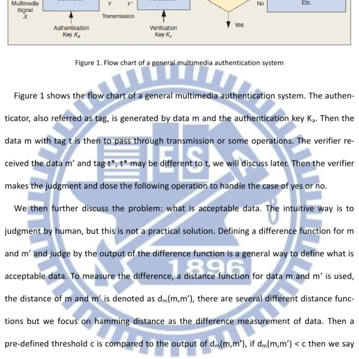
Figure 1. Flow chart of a general multimedia authentication system

Figure 1 shows the flow chart of a general multimedia authentication system. The authen-ticator, also referred as tag, is generated by data m and the authentication key Ka. Then the

data m with tag t is then to pass through transmission or some operations. The verifier re-ceived the data m’ and tag t*, t* may be different to t, we will discuss later. Then the verifier makes the judgment and dose the following operation to handle the case of yes or no.

We then further discuss the problem: what is acceptable data. The intuitive way is to judgment by human, but this is not a practical solution. Defining a difference function for m and m’ and judge by the output of the difference function is a general way to define what is acceptable data. To measure the difference, a distance function for data m and m’ is used, the distance of m and m’ is denoted as dm(m,m’), there are several different distance

func-tions but we focus on hamming distance as the difference measurement of data. Then a pre-defined threshold c is compared to the output of dm(m,m’), if dm(m,m’) < c then we say

m’ is acceptable as the ground truth.

The wrong judgments made by verifier may have two different types. One is the data is acceptable but the judgment rejects the data, we referred this type as a false alarm. The other one is the data is unacceptable but the judgment authenticates the data, we referred this type as a false positive.

14

In a soft authentication scheme, only one threshold c to define the acceptableness is not enough since it is difficult to distinguish data with difference around threshold c. As for the main goal of soft authentication, we should also give the freedom when data with difference around threshold t. Thus, we define two thresholds c1, c2, where c1 is the threshold of

ac-ceptable difference ratio of data m and c2 is the threshold of unacceptable difference ratio

of data. We denote dm(m,m’) asδm,

ifδm < c1, then m’ is acceptable,

ifδm > c2, then m’ unacceptable,

if c1 ≦δm ≦ c2, m’ can be accepted or reject without penalty.

The region between thresholds c1, c2 are the freedom region, the message can be

accept-ed or rejectaccept-ed without punishment, this give the freaccept-edom when authentication and also conform to the nature of soft authentication.

The measurement of an AMAC is to consider the punishments of the two types: false alarm and false positive,

the probability of false alarm = P[ Reject|δm < c 1]

the probability of false positive = P[ Pass|δm > c2 ]

In general, there are two ways to compare two different AMACs. One is to set the param-eters of both AMACs to comparing them under the same level of false alarm, the AMAC has a lower probability of false positive is better than the other. We also can compare them un-der the same level of false positive. Another way is to define an objective function to com-pute the total penalty, for example:

15

penalty = a1* P[Reject|δm < c1] + a2* P[Pass|δm > c2]

Where a1, a2 are different penalty coefficients for false alarms and false positives.

3.2 The Error model of tag

In the previous section we had mentioned that the verifier may receive a tag t* which is different to the correct tag t. The length of tag often is short in the authentication scheme, 128 bits to 1024 bits is a suitable range of tag lengths. Consider that the multimedia message with a small portion of errors, it is reasonable that the AMAC tag may have errors, too. To deal with this problem, one solution is to assume that the AMAC tag is always correct after the verifier received the modified data. This assumption can be true in the situation that er-rors only occur in data not tag or when the AMAC tag protected by an error-correcting code. The other way is assumed the AMAC tag also has errors, then the accuracy of AMAC will de-crease compared to AMAC tag with no errors. We assume the AMAC tag is correct in the rest of our paper.

3.3

The error model of messages

We assume the error probability of a message is randomly and independently, the loca-tions of error occur are not correlated. This assumption can simplify the problem model without loss generality. The error models of message are different under different circum-stances like forgery, compression, watermarking, channel noise… etc. In different applica-tions and environments, we can just adjust the threshold parameters of AMAC to find a suitable authentication scheme, and the random sampling model can make the error model fit the random error distribution condition. We also assume the verifier has information of

16

the error model without loss generality.

3.4

Definitions of AMACs

In this section, we will first define the model of MAC in math, and then introduce the definitions of AMAC in [18] and our AMAC definitions with the authentication model. Then we compare the two different models and describe the reason we use our definitions. At the least of this chapter, we will discuss the probabilistic properties of AMAC.

3.4.1

Definitions of MACs

Let the integer s be a security parameter. A message authentication code (MAC) is a triple (K, T, V), where algorithms K, T, V run in time polynomial and satisfy the following syntax. The key generation algorithm K takes as input a random string and returns a secret key k of length s. The authenticating algorithm T takes a message m and a secret key k as inputs and produces a string tag t. The verifying algorithm V takes a message m’, a secret key k and a string tag as inputs and returns a value {1,0}. A MAC has to satisfy a correctness requirement: After k is generated by K and tag is generated by T, V on the input (m’, t), outputs 1 if m’=m.

3.4.2 AMAC with parameters (s, d

, e, α), algorithms (K, T, V)

Let the integer s be a security parameter, algorithms K, T, V run in time polynomial, the key k is generated by algorithms K with length s. d is the distance function of messages witch d(m,m’) return the distance of m with m’, d can be Hamming distance or other distance func-tion.

17

if tag is generated using algorithm Tk on input message m, then algorithm Vk, on

in-put(m’,tag) , outputs 1 with probability at leastα, if dm(m, m’)≦e. Here e stands for the

ac-ceptable number of errors.

From the above definition, we can observe that an AMAC is a probabilistic guarantee such that if the number of errors blows to e, than the AMAC make the correct decision only at least αprobability, which is quite different to the probabilistic guarantee of cryptographic MAC. Also from the above definition, it does not consider the situation that when too many errors occur and should not be accepted by the verifier, there is no probabilistic guarantee that the AMAC can detect the errors, because of the insufficiencies of the AMAC definition above, we enhance the AMAC later.

3.4.3 AMAC with parameters(s,d

,c

,c

,p

,p

), algorithms (K,T,V)

Different from the AMAC definition in 3.4.2, the original error threshold e becomes two error thresholds c1, c2, and the probability parameter e also becomes two probability

param-eters p1, p2. The main idea is to consider the probability AMAC outputs 1 of both situations:

acceptable number of errors and unacceptable number of errors.

Let the integer s be a security parameter, algorithms K, T, V run in time polynomial, the key k is generated by algorithms K with length s. d is the distance function of messages witch dm(m, m’) return the distance of m with m’, d can be Hamming distance or other distance

function. c1, c2 are two parameters of errors, they can be real numbers between 0 and 1 or a

natural number of errors, depends on the distance function dm. p1, p2 are two probabilities

which satisfy 0≦ p1<p2≦1. The following two requirements are satisfied:

) 1 ( ] 1 ) ' , ( [ ) ' , (m m c₁then P V t m   p₁ d if _{m k}

18

T is the tag algorithm which t=T(k, m), V is the verification algorithm which on input (t, m’) outputs 1 with probability p≧p1 if d(m, m’) ≦ c1 and outputs 1 with probability p ≦ p2 if

d(m, m’) ≧ c2, which means when the number of errors below some threshold c1, the

veri-fication should pass greater then a high probability p1. On the other side, when the number

of errors above some threshold c2, the verification should pass under then a relatively lower

probability p2.

Compare to AMAC definition in 3.4.2, the definitions here are more suitable to real world application since both false alarms and false positives will have cost for the verifier.

3.4.4 Distance-preserving AMACs

Distance-preserving is a key idea of reducing the distance estimation of message to the distance of tags. We will introduce how to use the information of tags to estimate the dis-tance between the messages later.

A (dm, dt, δm, δt)-distance-preserving AMAC satisfy the following:

For any m1,m2, such that dm(m1, m2) ≦ δm, the expected value of dt(t1, t2) ≦δt, we will

use the properties of distance-preserving AMACs to construct AMACs with definition of 3.4.3. A straightforward idea to construct V(t, m’) is:

return 1 if dt(t, t’) ≦ 2δt, return 0 otherwise.

This verification function will satisfy (1) with p1 = 1/2, c1 = δm, but (2) is not satisfied,

since we don’t know p2 and how to decide c2. Our idea is if we know the distribution of

) 2 ( ] 1 ) ' , ( [ ) ' , (m m c₂then P V t m   p₂ d if _{m k}

19

Et(δm) then we can compute the expected p1 and p2 given c1, c2.

3.5 Mutually independent AMACs

For the reason that we want to know the distribution of Et(δm), we use AMACs with

in-dependent symbols .An lm -dimension message space with alphabets N constructed from all

possible messages of length lm. One of the values {0,…, N-1} is assigned to each dimension,

such that the message space contains N^ lm possible messages. We compute each AMAC

symbol with non-overlapping sets of message. Given a key k and an initialization vector I, the N-ary AMAC algorithm maps each message to an AMAC tag of length L. The following theo-rem holds:

Assume the existence of a pseudo-random generator, AMAC symbols are mutually inde-pendent.

When we calculate an AMAC tag of length L, a message is partitioned into L non-overlapping sets after the operations with the outputs of PRG, the pseudo-random number generator. Each set contains lm /L elements. Each AMAC symbol is calculated from

the corresponding set. Since the random sampling and modulo operations eliminate the correlations between each set, the AMAC symbols are mutually independent.

20

3.6 Probabilistic properties of mutually independent AMACs

If an AMAC is mutually independent, then the probabilistic properties of an AMAC tag changes can decide the properties of AMAC. We denote the probabilistic properties of an AMAC tag changes as PA, thenδt can be written as a binomial distribution of PA.

Where PA can be written as a function ofδm, PA will increase strictly when δm increase as

the distance-preserving property. Two different values ofδm will produce two different

bi-nomial distributions.

Figure 2. δm with different number of errors.

0 50 100 150 200 250 300 350 400 450 0 5 10 15 20 25 30 35 40 45 50 55 60 error=0.01 error=0.02 δt times x L A x A L x t m m d m A A

P

P

C

x

t

t

d

P

f

P









)

1

(

]

)

'

,

(

[

)

(



21

Chapter 4

Our AMAC Algorithm

Our AMAC is a probabilistic checksum calculated by using pseudo-random permutation, masking via a modulo sum operation, and MODE function, such that a small difference be-tween the two messages tends to result in a small difference bebe-tween their AMACs. N is the symbol size of messages, for any messages we can change N easily depending on the verifier. For N=2, the N-ary AMACs reduces to the binary AMACs where modulo sum operator reduc-es to XOR operation and MODE function reducreduc-es to MAJORITY function.

Let m be the input N-ary message of length lm. The ith element in the message is denoted

as m(i). Given a secret key k generated by K and a pseudo-random number generator PRG. As with conventional MACs, the length of AMACs L is typically chosen in the range 128≦ L ≦ 1024 bits. We compare different AMACs with the same length L, or we say an AMAC is better than the other if they have the same properties while one has shorter L.

22

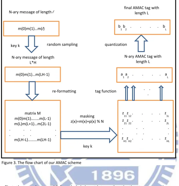
First, the row data m with length l is input into authentication tag generation, random sampling is taken to reduce the size of m from l to L*H. After re-formatting, the matrix M is masked by random matrix P generated with key k. The matrix Z then input to the tag function column by column, the output after quantization is the final AMAC tag with L bits.

N-ary message of length L*H matrix M m(0)m(1)…..…m(L-1) m(L)m(L+1)…m(2L-1) . . . . . . . . m(LH-L)………m(LH-1) m(0)m(1)…m(LH-1) re-formatting m(0)m(1)…m(l)

N-ary message of length l

random sampling z 11z12 . . . . z1L z 21z22 . . . . z2L . . . . . . . . z H1zH2 . . . . zHL masking z(x)=m(x)+p(x) % N . . . tag function a 1 a2 . . . . aL

N-ary AMAC tag with length L b

1 b2 . . . . bL

quantization

final AMAC tag with length L

key k

key k Figure 3. The flow chart of our AMAC scheme

23

4.1 Initialization

Verifier and owner share the secret key k, k is input to the Pseudo-Random Generator (PRG) as a seed. The output of PRG must be available to both verifier and owner. PRG is used repeatedly as a source of N-ary pseudo-random numbers.

4.2 Feature extraction

A feature vector that represents the media content extracted from the original message and hashed into a small digest. The digest is then signed by a standard digital signature algo-rithm. Since only the semantic information is extracted for authentication, the incidental noise can be tolerated. Different features could be used to represent the content of the im-age such as edge information, DCT coefficients, and color or intensity histogram, histogram feature was used in our AMAC.

In our AMAC, only the error number can detect, not the perceptual data error. If the at-tacker changed the data with the amount of errors that blows the threshold, he will not be detected by our AMAC since the amount of errors is acceptable. In our AMAC, the error posi-tion and error distance are not measured in the tag funcposi-tion. The histogram feature of data only considers the number of errors. To enhance our AMAC for detecting attacker, prepro-cessing the multimedia data to extract the perceptual feature is helpful. There are many works that extract different types of multimedia data features, we make the assumption that the extract features are suitable for further histogram feature extraction, which means the errors in features of multimedia are not location and distance correlated. Thus, we can apply feature extraction of the type of multimedia data and then apply our AMAC, the final AMAC can detect the attacker.

24

4.3 Random sampling

For the reason that the decrease of accuracy of AMAC is not as much as the decrease of proportion of message which take part in the computation of AMAC, so we use random sampling to reduce the computation.

We use m_old to denote the original message with length l, L is the length of the tag, and namely, the tag has L symbols. We sample L*H symbols from the original message by using PGR. The other message symbols are not taking part in the computation of AMAC.

The PRG is used to form a sample table such that each element in the message matrix and in the sample table forms a new matrix accordingly. The verifier and the message sender use the shared key k for PRG. The purpose of the pseudo-random sampling is to not only destroy any existing spatial correlation within the neighboring elements but also enhance the securi-ty against attack.

25

4.4 Masking

The N-Nary message of length L*H, denoted asm(m(0),m(1),...,m(LH1), Then the message re-formatted into a matrix, denoted as

M=

Let P be the pseudo-random L*H matrix generated from PRG. The matrix M is then masked by a modulo N operator with the pseudo-random matrix P, element by element. Denote the masked matrix M as M=(M+P)N, where mij=(mij+pij) module N.

The modulo operation leads to the variables , which are independent of each other and unbiased whenever the samples {pij} are mutually independent and unbiased which means

they obey a discrete uniform distribution on {0,1,…,N-1}.

m(0)m(1)…..…m(L-1) m(L)m(L+1)…m(2L-1) . . . . . . . .

26

4.5 Feature extraction: Tag function

After random sampling and masking, then the tag t of length L symbols is computed by matrix M, t=Tag(M). Because of random sampling, we can simply divide M into rows to com-pute each tag symbol without permutation. Each tag symbol is comcom-puted by ti=Tag(Mi),

Mi={mi, mL+i,…, mL(H-1)+i}, thus each tag symbol is mutually independent.

MODE

The MODE is defined as the most common value in a set. If a “tie” occurs, the MODE op-eration breaks the tie by comparing the adjacent values.

Example:

MODE(0, 1, 1, 1)=1, MODE(1, 3, 0, 3, 2)=3

MODE2

The MODE2 is defined as appearance frequency of the most common value in a set. If a “tie” occurs, the MODE operation breaks the tie by comparing the adjacent values.

27

4.6 Feature reduction: Quantization

Quantize the tag symbol into binary or other n-nary, n<N, can reduce the bits of tag while not affect the accuracy of AMACs significantly. The reason is that if we quantize the tag sym-bols, the same length of tag can contain more symbols.

Example:

tag t=(0, 1, 2, 3), Quantization(t, 2)=(0, 1, 0, 1)

More symbols can affect the accuracy significantly in nature. But if we fix the length of the tag, the only way to increase the number of symbols is to compress each symbol. The disad-vantage is that the probability of each tag symbol change is decreased, for example:

mi=(0, 1, 2, 3, 3)

Tag(mi) = ti = 3

After transmission, mi becomes to mi’=(0, 1, 2, 3, 1)

Tag(mi’) = ti’= 1, where ti ≠ ti’

After quantization, ti = Quantization(ti,2) = 1,and the value of ti’ becomes to

ti’ = Quantization(ti’,2) = 1 is equal to ti, in such cases, the tag is not changed if we quantize

the tag.

The effect of quantization will have the benefit of accuracy since the number of symbols is increased, but the probability of each tag symbol change is decreasing, the final AMAC accu-racy is the tradeoff of the two factors.

28

Figure 4. False alarm versus true positive for different quantization

From above figure 6, we can observe that with the same condition but different quantization parameter, more quantization has better accuracy in these three cases.

0 0.1 0.2 0.3 0.4 0.5 0.6 0.7 0.8 0.9 1 0 0.2 0.4 0.6 0.8 1 MODE2 s=0.06, q=2 MODE2 s=0.06 q=4 MODE2 s=0.06 q=16

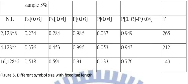
29 sample 3% N,L Pa[0.03] Pa[0.04] P[0.03] P[0.04] P[0.03]-P[0.04] T 2,128*8 0.234 0.284 0.986 0.037 0.949 265 4,128*4 0.376 0.453 0.996 0.053 0.943 212 16,128*2 0.518 0.591 0.91 0.133 0.776 143

Figure 5. Different symbol size with fixed tag length

From figure 7, we use the same bit length of the tag but different symbol size without quan-tization, although small N seems to have better performance but in the case N=2 compares to N=4, the AMAC with N=2 are not significantly dominate the AMAC with N=4. This means that the AMAC is not always benefit if we quantize the AMAC symbols more. A practical way is to find the best quantization factor for the AMAC with experiments.

30

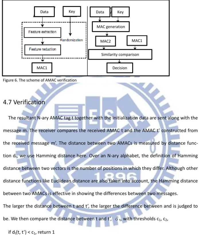
4.7 Verification

The resultant N-ary AMAC tag t together with the initialization data are sent along with the message m. The receiver compares the received AMAC t and the AMAC t’ constructed from the received message m’. The distance between two AMACs is measured by distance func-tion dt, we use Hamming distance here. Over an N-ary alphabet, the definition of Hamming

distance between two vectors is the number of positions in which they differ. Although other distance functions like Euclidean distance are also taken into account, the Hamming distance between two AMACs is effective in showing the differences between two messages.

The larger the distance between t and t’, the larger the difference between and is judged to be. We then compare the distance between t and t’, δt, with thresholds c1, c2,

if dt(t, t’) < c1, return 1 if c1≦ dt(t, t’)≦c2, don’t care if dt(t, t’)>c2, return 0 MAC1 MAC2 MAC1 MAC generation Data Data Similarity comparison Key Key Decision Figure 6. The scheme of AMAC verification

31

Tag Algorithm

input: the secret key k, data m, sample rate s, L, H

1 generate index set a, where ai = PRNG(k,i), i from 0 to LH - 1

2 m = (ma0, ma1,…, maLH-1)

3 generate r, where ri = PRNG(k, i + LH), i from LH to 2LH - 1

4 m = m + r

5 mi = (mi, m2H+i,…, m(L-1)H+i)

6 t = (MODE2(m0), MODE2(m1),…, MODE2(mL-1))

7 return t

s

Verification Algorithm

input: the secret key k, modified data m’, tag t, thresholds c1,c2

1 t’ = Tag(m’, k) 2 δt = dt(t, t’) 3 if dt(t, t’) < c1, return 1 if c1≦ dt(t, t’) ≦ c2, don’t care if dt(t, t’) > c2, return 0 s

32

Chapter 5

Experiment

5.1

Experiment environment

We use an 8-bit 800*600 image as our example, the row data can be seen as a gray-scale image, and the desired AMAC length is 128 bits to 1024 bits. We use the computer with Intel Core i7 Q720 1.6GHz CPU and 4GB RAM and coding with Bloodshed Dev-C++ 4.9.9.2. The key is generated as the seed for the pseudo random number generator. In this chapter, we will first discuss the comparison for two different AMACs, then discuss several factors that affect to our AMAC and compare to the AMAC of [18]. The distance function we use for data and tags are hamming distance, which is the number of differences of each symbol, the distance of each symbol is not considered in our AMAC.

33

5.2

Comparison of two different AMACs

To compare two different AMACs, we compare the probability of each AMAC outputs the correct authentication given the same input data, the keys of AMACs are generated randomly. We simulated the authentication many times with different keys and compute the probabil-ity that the AMAC make the correct authentication decision. The error added to the image are randomly for each byte, for example, a pixel with original value 100 are randomly changed to 0~255 except 100 if the error occurred to this pixel. The amount of errors added to the image is just at the edge of the acceptable number of errors or the unacceptable number of errors, we will discuss this later.

5.2.1 The length of AMAC tag

It is not difficult to see that an AMAC with longer tag take advantage over the other with shorter tag on distinguishable abilities. Suppose we compare two AMACs with the same AMAC family, one with 128-bit length tag and the other with 256-bit length tag, and the 256-bit AMAC divided into two partitions. The first 128 bits are the same as the 128-bit AMAC tag, and the later 128 bits are additional information that does not contains in 128-bit AMAC tag. Consider the worst case of 256-bit AMAC, we just drop the later 128 bits, the output result of authentication is the same as the 128-bit AMAC, thus the distinguishable abilities of the 256-bit AMAC is equal or better than the 128-bit AMAC. In addition, the long-er the tag is, the probability of tag long-error increase, or we need more efforts and redundancy to protect the tag. Thus to compare AMACs fairly, we compare them under the same length of AMAC tag.

34

5.2.2 AMAC distinguishable ability measurement

We measured an AMAC with the distinguishable ability which is defined as follows: P1 = P [m’ pass AMAC verification | m’ is acceptable]

P2 = P [m’ pass AMAC verification | m’ is unacceptable]

Comparing two AMACs at the same level of P2, the AMAC with higher P1 has more advantage

than the other.

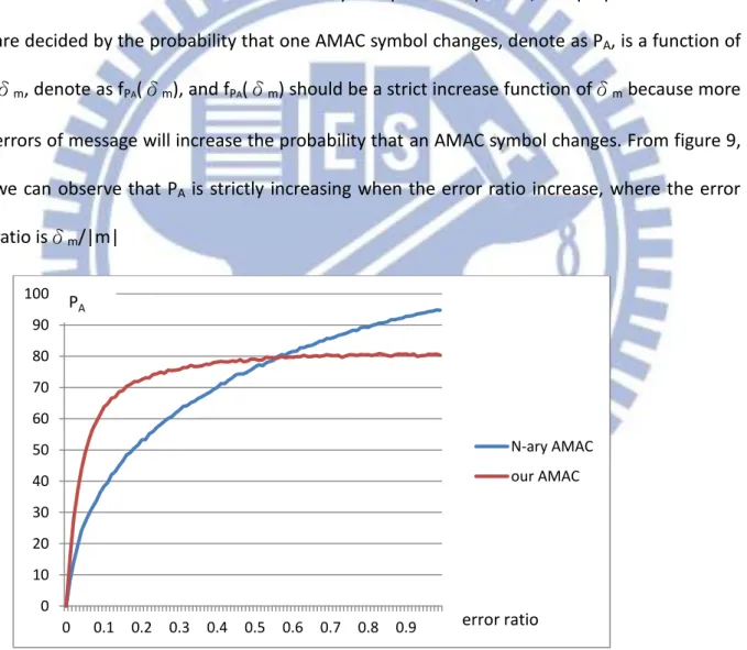
Since we consider AMACs with mutually independent symbols, the properties of AMAC are decided by the probability that one AMAC symbol changes, denote as PA,is a function of

δm, denote as fPA(δm), and fPA(δm) should be a strict increase function ofδm because more

errors of message will increase the probability that an AMAC symbol changes. From figure 9, we can observe that PA is strictly increasing when the error ratio increase, where the error

ratio isδm/|m|

Figure 7. The probability that one AMAC symbol changes under different error ratio 0 10 20 30 40 50 60 70 80 90 100 0 0.1 0.2 0.3 0.4 0.5 0.6 0.7 0.8 0.9 N-ary AMAC our AMAC error ratio P_A

35

Since the AMAC symbols of ours are independent, the expected total number of tag sym-bol changes E(δt) can be simply calculated by LPA. And we define the accuracy of AMAC:

accuracy = P[true positive] – P[false alarm]

where P[true positive] = P[true positive |δm = c1],

P[false alarm] = P[false alarm |δm = c2]

The accuracy we defined is simply. Consider the penalty describe below: penalty = a1* P[Reject|δm < c1] + a2* P[Pass|δm > c2]

where a1, a2 are different penalty coefficients for false alarms and false positives

Since we does not know the true environment data error probability and distribution, we can not decide the coefficients of a1, a2. We assume a1 = a2, then the penalty becomes:

penalty = a1* (P[Reject|δm < c1] + P[Pass|δm > c2])

And we remove the factor of a1

penalty = P[Reject|δm < c1] + P[Pass|δm > c2]

which equals to P[false alarm] + P[false positive],

1 - penalty = 1 - P[false positive] - P[false alarm] = P[true positive] – P[false alarm] Thus, 1 - penalty = accuracy

36

5.3 Error estimation with tags

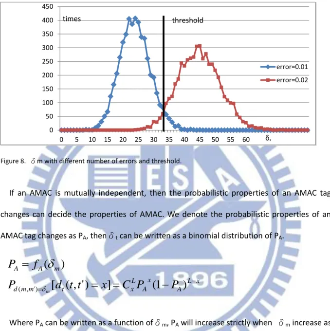
Figure 8. δm with different number of errors and threshold.

If an AMAC is mutually independent, then the probabilistic properties of an AMAC tag changes can decide the properties of AMAC. We denote the probabilistic properties of an AMAC tag changes as PA, thenδt can be written as a binomial distribution of PA.

Where PA can be written as a function ofδm, PA will increase strictly when δm increase as

the distance-preserving property. Two different values ofδm will produce two different

bi-nomial distributions.

Figure 10 shows an example where the acceptable data errors is 1% and the unacceptable data error is 2%, and both 1% errors data and 2% errors data are generated 5000 times, and compute the number of result δt. Data with 2% errors are generally having higher value of δt

which is consist to our expectation.

0 50 100 150 200 250 300 350 400 450 0 5 10 15 20 25 30 35 40 45 50 55 60 error=0.01 error=0.02 δt times _threshold x L A x A L x t m m d m A A

P

P

C

x

t

t

d

P

f

P









)

1

(

]

)

'

,

(

[

)

(



37

From figure 10, there exist overlap region of 1% errors and 2% errors. This means no mat-ter what threshold we use in this case, there exists probability that the authentication deci-sion made by threshold not correct is not equal to 0.

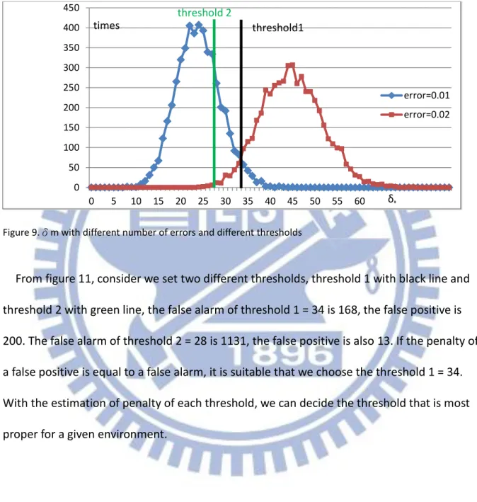
Figure 9.δm with different number of errors and different thresholds

From figure 11, consider we set two different thresholds, threshold 1 with black line and threshold 2 with green line, the false alarm of threshold 1 = 34 is 168, the false positive is 200. The false alarm of threshold 2 = 28 is 1131, the false positive is also 13. If the penalty of a false positive is equal to a false alarm, it is suitable that we choose the threshold 1 = 34. With the estimation of penalty of each threshold, we can decide the threshold that is most proper for a given environment.

0 50 100 150 200 250 300 350 400 450 0 5 10 15 20 25 30 35 40 45 50 55 60 error=0.01 error=0.02 δt times _threshold1 threshold 2

38

5.4 The effect of different sample rate

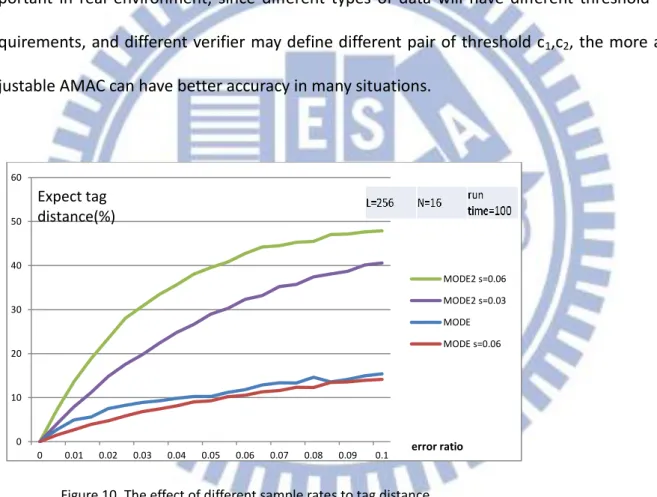
To choose the appropriate sample rate is a key of our AMAC, we compare the effect of different sample rates on the difference between tags. We can see from figure 12, higher sample rate will cause the probability PA increase in both MODE1 and MODE2, and MODE2

has higher value of E(δt ) and the line changes significantly when the sample rate changes

from 0.03 to 0.06. We can conclude that MODE2 is more adjustable. The adjust ability is im-portant in real environment, since different types of data will have different threshold re-quirements, and different verifier may define different pair of threshold c1,c2, the more

ad-justable AMAC can have better accuracy in many situations.

Figure 10. The effect of different sample rates to tag distance 0 10 20 30 40 50 60 0 0.01 0.02 0.03 0.04 0.05 0.06 0.07 0.08 0.09 0.1 MODE2 s=0.06 MODE2 s=0.03 MODE MODE s=0.06 error ratio Expect tag distance(%)

39

Figure 11. The accuracy comparision of different size of N

The figure 13 shows the accuracy comparison of different size of N for N=16 and N=256, different from the work [18], we find that not greater N will have better accuracy because if we increase the size of N the number of symbols take part in the tag function will decrease and the number of symbols of tag will also decrease. The work [18] didn’t consider the tag length should be fixed in bits. With experiments, we found that N=16 has better accuracy in general, so we set N=16 in our experiments.

0 0.2 0.4 0.6 0.8 1 1 11 21 31 41 51 61 71 AMAC2 N=256 AMAC2 N =16 true positive - false alarm threshold

40

5.5 Accuracy comparison of different tag function

H0: message is authentic

H1: message is not authentic

p1: TP / (TP + FN)

p2: FP / (FP + TN)

H0: d(m, m’) / |m| > r1

H1: d(m, m’) / |m| ≦ r2

Figure 12. The accuracy comparison of different AMACs

We compare p1 at the same level of p2, from figure 14 we can see that AMAC with MODE2

has advantages of both sample rates 0.06 and 0.12 in the AMAC with MODE, sample rate=0.12. In figure 14 we can also examine the idea that higher sample rates not ensure better performance of accuracy. AMAC with MODE2 sample rate=0.06 is dominated AMAC with MODE2 sample rate=0.12 at every different level of p2.

0 0.1 0.2 0.3 0.4 0.5 0.6 0.7 0.8 0.9 1 0 0.1 0.2 0.3 0.4 0.5 MODE2 s=0.06 MODE2 s=0.12 MODE s=0.06 p1 p2 truth decision

41 Figure 13. The effect of threshold to accuracy

From the above figure 15, the green line shows the difference of P[0.01] - P[0.04], and the value is maximized when the threshold is equal to 11.

Figure 14. AMACs comparison for error rate c1=0.01, c2=0.03

0 0.2 0.4 0.6 0.8 1 1.2 1 2 3 4 5 6 7 8 9 10 11 12 13 14 15 16 17 18 19 20 21 22 23 24 25 26 27 28 N-ary AMAC Our AMAC threshold accuracy threshold accuracy

42

5.6 Effect of different thresholds

Figure 15. Effect of different thresholds

From above figure 17, when the threshold is blowing 30, data with error rate both 3% and 4% cannot pass the authentication, and when the threshold is greater than 90, data with er-ror rate both 3% and 4% can pass the authentication almost 100% probability. When thresh-old between 30 and 90, data with error rate both 3% and 4% have a different pass authenti-cation probability, thus can distinguish the data error. We can observe that the threshold close to 55 have the largest probability difference.

0 0.2 0.4 0.6 0.8 1 1.2 1 6 11 16 21 26 31 36 41 46 51 56 61 66 71 76 81 86 91

AMAC,1000times,800*600,0.03

43

5.7 Effect of quantization

Figure 16. The accuracy of different quantization

Quantize the tag symbol into binary or other n-nary, n<N, can reduce the bits of tag while not affect the accuracy of AMACs significantly. The reason is that if we quantize the tag sym-bols, the same length of tag can contain more symbols. From above figure 18, we compare different values of q, for q = 2, q = 4 and q = 16, and fix the length of tag with 256 bits. For q = 2, there are 256 tag symbols, for q = 4, there are 128 tag symbols, and for q = 16, there are 64 tag symbols. We can observe that in the same condition and fixed length of tag but dif-ferent quantization parameter, more quantization has better accuracy in this case.

0 0.1 0.2 0.3 0.4 0.5 0.6 0.7 0.8 0.9 1 0 0.2 0.4 0.6 0.8 1 MODE2 s=0.06, q=2 MODE2 s=0.06 q=4 MODE2 s=0.06 q=16

44 Figure 17. Our AMAC with different quantization

More symbols can affect the accuracy significantly in nature. But if we fix the length of the tag, the only way to increase the number of symbols is to compress each symbol. The disad-vantage is that the probability of each tag symbol change is decreasing, from figure 19 we can observe that there exist upper bounds for both q = 2 and q = 16, this is because when the error ratio close to 1, the data is changed extremely and seems like a new data, so as the final tag. Thus, the probability of each tag symbol change is bounded by 1/q.

0 10 20 30 40 50 60 70 80 90 0 0.1 0.2 0.3 0.4 0.5 0.6 0.7 0.8 0.9

our AMAC with q=2 our AMAC with q=16 distance of

tags

45

5.8 Accuracy under different condition

Figure 18. Accuracy of our AMAC

We experiment the accuracy of our AMAC of MODE2 with the acceptable error rate c1=0.01 and unacceptable error rate c2=0.02, and compare the accuracy performance under

different threshold parameter of AMAC. Setting different threshold we have several pairs of (p1,p2), the second pair (0.986,0.013) shows that the AMAC can distinguish both c1 and c2

data error rate with about 98.5% of accuracy.

0.94 0.95 0.96 0.97 0.98 0.99 1 1.01 0 0.2 0.4 0.6 0.8 p 1 p 2

46 Figure 19. Different error condition

From figure 21 we can observe that compare to the error parameters with c1=0.01, c2=0.02

has better accuracy than to distinguish the error parameters with c1=0.03, c2=0.04. The

rea-son is that for c1=0.01, c2=0.02, the number of errors of c1 are twice than the number of

er-rors of c2. But in the case of c1=0.03, c2=0.04, the number of errors of c1 are only 1.33 times

than the number of errors of c2, so we can expected the average distance of tags is about

only 0.33 times compares to the error parameters with c1=0.01, c2=0.02. Thus it is more

dif-ficult to distinguish error of 0.03 and 0.04. The tag length should be longer to reach the same level of accuracy as error parameters with c1=0.01, c2=0.02.

0 0.2 0.4 0.6 0.8 1 1.2 0 0.2 0.4 0.6 0.8

MODE2 s=0.06, c1=0.03,c2=0.04

47

5.9 Comparison of computation time

We compare the computation with different sample rate. The computation time is defined as the time to compute an AMAC tag. The data size we use is 800*600 bytes. Sample rate = 0.03 the computation time is 7ms, and when the sample rate is 0.06, the computation is 11ms, which is not as twice as 7ms. Moreover, consider the sample rate = 1, which means total data are used to compute the AMAC tag and no sampling was used, the computation time is only 15ms, not linear growth with the sample rate. We found that with random sam-pling, most of computation time is using on the random number generation for the position that random sampling need. If we eliminate the time used on random number generation, sample rate = 0.03 the computation time is 1ms, and when the sample rate is 0.06, the computation is 1ms, sample rate = 1 is 15 ms. The result computation time is close to linear with the sample rate, as we expected. We use the pseudo random function of c++, more effi-cient pseudo random function can increase the performance, still the benefit of random sampling is restrict by the pseudo random generation.

with random table

computation time for a AMAC tag, data size = 800*600 bytes

48

Chapter 6

Security analysis and discussion

The AMAC construction already satisfies some kind of security property. Assume that the construction is distance-preserving, for some distance functions and parameters. Then con-sider an adversary trying to produce two messages m1, m2 such that dm(m1, m2) > c2 , and the

key k has been generated using the key-generation algorithm. An adversary tries to convince a verifier that the same tag is valid for both m1 and m2, which means Verification of m2 with

the tag t1=T(m1) pass with higher probability than p2. However, since the k is generated

ran-domly and the attacker has no information about the key, the attacker must cannot know which positions of data are chosen to compute the tag. Without any information of the posi-tion chooses, the attacker chooses the posiposi-tions seems randomly from the perspective of the verification. The only way to broken the security is to break the key or pseudo random num-ber generation.

For the perceptual data attack, the attacker changed the data within the acceptable amount but not randomly, the multimedia data is not the same from human perspective. In our AMAC, only the error number can detect, not the perceptual data error. If the attacker

49

changed the data with the amount of errors that blows the threshold, he will not be detect-ed by our AMAC. The error position and error distance are not measurdetect-ed in our tag function. To enhance our AMAC for detecting attacker, preprocessing the multimedia data to extract the perceptual feature is helpful. There are many works that extract different types of mul-timedia data features, we make the assumption that the extract features are suitable for further histogram feature extraction, which means the errors in features of multimedia are not location and distance correlated. Thus, we can apply feature extraction of the type of multimedia data and then apply our AMAC, the final AMAC can detect the attacker.

50

Chapter 7

Conclusion

We proposed an AMAC with sensitivity control that can well adjust to different error thresholds, and consider the nature of AMAC using random sampling to reduce the compu-tation time of AMAC. We experiment our AMAC and compare to others, the results show that our AMAC has advantages than the others. However, to distinguish forgeries from inci-dental errors, we need to combine our AMAC with robustness preprocessing to keep the features of multimedia data. To enhance the robustness and combine with techniques of multimedia data preprocessing are future works.

51

References

[1] Emin Martinian and Gregory W. Wornell, “Multimedia content authentication:

fundamental limits,” in IEEE International Conference of Image Processing, Rochester, NY, Sep. 2002, vol. 2, pp. 22–25.

[2] Bin B. Zhu, Mitchell D. Swanson, and Ahmed H. Tewfik, “When seeing isn’t believing: Current multimedia authentication technologies and their applications,”

in IEEE Signal Processing Magazine, pp. 40–49, Mar. 2004.

[3] Chai Wah Wu, “On the design of content-based multimedia authentication

systems,” in IEEE Transactions on Multimedia, vol. 4, no. 3, pp. 385–393, Sep. 2002. [4] Richard Graveman and Kevin E. Fu, “Approximate message authentication codes,” in

Ad-vanced Telecommunications & Information Distribution Research Program, vol. 1, Col-lege Park, MD, Feb. 1999.

[5] C Kailasanathan, R Safavi-Naini, and P Ogunbona, “Image authentication surviving acceptable modifications,” in IEEE-EURASIP Workshop on Nonlinear Signal Image Processing, Baltimore, MD, Jun. 2001.

52

[6] M. Kıvanc Mıhcak and Ramarathnam Venkatesan, “A tool for robust audio information hiding: A perceptual audio hashing algorithm,” in International Information Hiding Work-shop, Philadelphia, PA, Nov. 2001.

[7] Liehua Xie, Gonzalo R. Arce, and Richard F. Graveman, “Approximate Image Message Authentication Codes,” in Collaborative Tech Alliance Communications and Networks, College Park, MD, pp. 217–221, Apr. 2003.

[8] Karen M. Bloch and Gonzalo R. Arce, “Analyzing protein sequences using signal analysis techniques,” in Computational and Statistical Approaches to Genomics,

pp. 113-124, 2003.

[9] Ashwin Swaminathan, Yinian Mao, and Min Wu,” Robust and Secure Image Hashing,” in IEEE Transactions on Information Forensics and Security, Vol. 1, No. 2, June 2006 [10]Marc Schneider and Shih-Fu Chang, “A robust content based digital signature for image

authentication,” in IEEE International Conference on Image, pp. 227-230, Sep. 1996. [11]Der-Chyuan Lou and Jiang-Lung Liu, “Fault resilient and compression tolerant digital

signature for image authentication,” in IEEE Transactions on Consumer Electron, vol. 46, no. 1, pp. 31–39, Feb. 2000.

[12]Ee-Chien Chang, Mohan S. Kankanhalli, Xin Guan, Zhiyong Huang, Yinghui Wu, “Robust image authentication using content based compression,” in ACM Multimedia System, vol. 9, pp. 121–130, Aug. 2003.

[13]Ching-Yung Lin, and Shih-Fu Chang, “A robust image authentication method

distinguishing JPEG compression from malicious manipulation,” in IEEE Transactions on Circuits System Video Technology, vol. 11, no. 2, pp. 153–168, Feb. 2001.