國
立
交
通
大
學
多媒體工程研究所
碩
士
論
文
基 於 空 間 時 間 最 佳 化 之 互 動 式 動 作 編 輯 系 統
An Interactive Motion Editing System
based on
Spacetime Optimization
研 究 生:藍英綬
指導教授:林奕成 助理教授
基 於 空 間 時 間 最 佳 化 之 互 動 式 動 作 編 輯 系 統
An Interactive Motion Editing System based on Spacetime Optimization
研 究 生:藍英綬 Student:Ying-Shou Lan
指導教授:林奕成 Advisor:I-Chen Lin
國 立 交 通 大 學
多 媒 體 工 程 研 究 所
碩 士 論 文
A ThesisSubmitted to Institute of Multimedia Engineering College of Computer Science
National Chiao Tung University in partial Fulfillment of the Requirements
for the Degree of Master
in
Computer Science
January 2009
Hsinchu, Taiwan, Republic of China
I
基於空間時間最佳化之互動式動作編輯系統
研究生:藍英綬
指導教授:林奕成 博士
國立交通大學
多媒體工程研究所
摘要
近年來動作捕捉技術被廣泛運用,然而錄製好的動作經常無法滿足更多需求。 爲了進一步擴增動作資料庫的多樣性,我們提出一個基於空間時間最佳化的互動 式動作編輯系統。藉由使用者控制各種限制條件,系統會根據這些條件調整原本 的動作合成出新動作。由於人體本身複雜的結構,很難使用控制器精凖地驅動各 個關節動作。因此我們避開困難繁雜的動力學計算,使用不同於完全物理模擬的 合成方式。我們將問題定義在關節旋轉所需角度的歐式空間上,再利用空間時間 最佳化的特性,可以輕易地控制各種人體運動上的限制條件。然而將二次規劃的 最佳化問題應用在人體結構上,會因為過多的關節和自由度造成花費大量的計算 時間在求解過程。於是我們觀察人體動作的連貫性,利用主成分分析捕捉最主要 的運動資訊,藉此減少問題的變量。最後我們再嵌入靜力平衡系統,提供一個直 覺而且簡單的控制方法,讓使用者能夠調整出栩栩如生的動作。II
An Interactive Motion Editing System
based on Spacetime Optimization
Student: Ying-Shou Lan
Advisor: I-Chen Lin
Institute of Multimedia Engineering
National Chiao Tung University
Abstract
In this thesis, we present an interactive motion editing system to synthesize new motions from an original input motion. The system adjusts the input motion in a strategy of consecutive short-term optimization by solving a quadratic program problem according to user-specified constraints. In contrast to fully physical simulation which is usually difficult to track joints forces accurately, we define our problem on the Euclidean space of joints angular configuration. Herewith we can exploit the advantage of spacetime optimization by supplying various kinds of kinematic constraints. However, to further alleviate the time-consuming computation, we reduce the number of variables by utilizing coherence of human motion. Finally, a static equilibrium system is embedded into the system to provide an intuitive and simple yet vital dynamics control.
Keywords: Motion Editing, Principle Components Analysis, Spacetime Optimization
III
IV
Acknowledgement
1. 首先要感謝父母對我的支持及幫助,讓我在求學過程中毫無後顧之憂,能夠 專心所學。 2. 指導教授 林奕成博士。感謝老師長久以來的耐心指導,在我遇到瓶頸時熱 心協助,不僅開拓我知識的視野,也使我逐漸瞭解思考解決問題的方法。 3. 實驗室的學長。其中任右學長對於我的個人研究犧牲自己的時間提供許多幫 助,昭自學長則是讓我領略到程式寫作的藝術。 4. CAIG 成員以及其餘同學,不論是日常生活中彼此照顧,或是學校作業 project 的合作,都讓我獲得成長的經驗。V
Contents
摘要 ... I Abstract ... II Special Acknowledgement ... III Acknowledgement ... IV 1 Introduction... 1 1.1 Motivation ... 1 1.2 Overview ... 2 1.3 Flowchart ... 4 2 Related Works ... 6 3 Methods ... 12 3.1 Segmentation ... 13 3.2 Kinematics Constraints ... 14
3.3 Equilibrium-based Force Response ... 17
3.4 Spacetime Optimization ... 20
3.5 Principle Components Analysis ... 22
3.6 Spline Interpolation ... 23
4 Experiments and Results ... 24
4.1 Weight of Continuity ... 24
4.2 Weights of Joints ... 26
4.3 Force Constants of Joints ... 26
4.4 Results ... 26
5 Conclusions and Future Works ... 31
VI
Figure 1: The flowchart ... 4
Figure 2: Algorithm outline of motion transformation ... 7
Figure 3: Kinematic character simplification: (a) elbows and spine are abstracted away, (b) upper body reduced to the center of mass, (c) symmetric movement abstraction ... 8
Figure 4: Error between a full-dimensional motion and the corresponding k-dimensional representation ... 9
Figure 5: The general angular and linear momentum pattern of a jumping motion ... 10
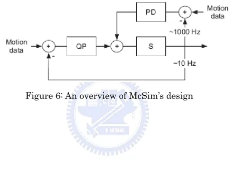
Figure 6: An overview of McSim’s design ... 11
Figure 7: Skeleton of human body ... 12
Figure 8: Each color for a segment ... 13
Figure 9: (left) Original motion, (right) adjusted motion satisfied the constraint ... 14
Figure 10: (left) Original motion, (right) adjusted motion satisfied the constraint ... 15
Figure 11: (left) Original motion, (right) adjusted motion satisfied the constraint ... 16
Figure 12: A spring and a damper assembled at the joint ... 17
Figure 13: Equilibrium ... 18
Figure 14: (left) Original motion, (right) adjusted motion satisfied the force constraint applied to the left limb of body ... 19
Figure 15: Relationshiop between accuracy and computation time ... 24
1
1 Introduction
1.1 Motivation
In recent years, using motion capture (MoCap) systems to animate humanoid 3D models has become more and more popular. MoCap data recording character’s motions are more realistic than key-frame based animations made by animators. However, to capture a set of motions is usually time-consuming and costs expensively. Besides, the recorded motion data are also difficult to directly apply to different environments and conditions. Thus, many researchers have devoted themselves to overcome these difficulties. Plenty of techniques have also been proposed, such as motion graph and space-time optimization. Both methods attempt to expand the variety of the original motion data set but through different ways: the former produces new motion by concatenating many smaller motion clips, while the later synthesizes a new one by adjusting an original motion to fit user-specified constraints.
The main limit of motion graph is that it cannot produce novel motion which is not originally in database. That is, the size of database decides the variety of synthesized motion. Moreover, maintaining the synthesis quality of a large motion database usually costs extremely. In contrast, spacetime optimization does not need a large database. With the underlying dynamics or kinematics model, it can synthesize more plausible results than key-frame interpolated motions. In other words, it can produce new motions which are
2
not limited by a database. However, the complexity of spacetime optimization itself is O
n
, where t is the number of iterations, and n is the number of degrees of freedom (DOFs). This leads the optimization process to be very inefficient when it is applied to highly dimensional human musculoskeletal model. For this reason, we propose to further improve the traditional optimization framework by decreasing the number of DOFs and simplifying the physical model, but keep it realistic as well.1.2 Overview
The base framework of our method is spacetime optimization, adjusting an original motion to fit user-specified constraints, including kinematic and force constraints. Nevertheless, the high complexity of human musculoskeletal model makes the optimization process time-consuming or difficult to converge to an acceptable solution. To overcome this problem, we observe that every human motion has considerable coherence. By the articulation of human skeleton, there is spatial relationship between neighbor joints; by the gravity and muscle force, there is temporal relationship between several frames. Therefore, we propose exploiting both spatial and temporal coherence to keep only the most effective dimensions.
Principle components analysis (PCA) is a space transformation technique by projecting multidimensional data sets to a lower dimensional space while retaining most significant features. When applying PCA on the motion data, it can hold the major moving information of the hierarchy. In
3
order to maximize the utilization of spatial coherence so that the moving information can be described more accurately in the low dimensional space, we divide each limb and torso into different segments and group the most correlated joints. As a result, we can use fewer DOFs to control the original motion properly in the optimization process. Temporal coherence makes the trajectories of motion vary continuously. We use splines to approximate the smooth of motion such that we only need to optimize key frames at regular intervals. Hereby, numbers of DOFs are further decreased in the phase of optimization.
Our editing system provides an interface for users to modify original motions by specifying high-level constraints, including kinematic constraints and force constraints. Kinematic constraints include end effectors positions, footsteps positions, etc. A force constraint is an external force applied to certain joints. Finally, the system iteratively adjusts the original motion to fit these constraints in the spacetime optimization process.
Instead of embedding fully physics-based model into our optimization framework, a simplified force response constraint is proposed, where we assume that the original and adjusted joint figures are both in a static equilibrium situation. We assemble springs at joints to exert muscle forces which counteract external forces. Without consuming time in extracting lots of physics parameters, we only have to project all muscle forces to the line of external force vector. By keeping each frame in static equilibrium, we can
simu
1.3
TheKin
Con
ulate the bFlowch
outline ofematics
nstraints
behavior ahart
f our meths
s
affected by hod is as fo FigureOrig
Seg
Low
S
Op
Res
4 y this exter ollows: e 1: The floginal Mo
gmentat
PCA
Dimens
Space
pacetim
ptimizat
sult Mot
rnal force owchartotion
tion
sional
me
ion
tion
plausibly.Equ
5
1. Divide the skeleton into different segments according to the loading BVH file.
2. Perform PCA on each segment respectively to transform the original moiton to a low dimensional space.
3. Embed the physical model in this low dimensional space. 4. Specify kinematic constraints and force constraints.
6
2 Related Works
It has been widely known that making character animation is a labor-intensive work. Instead of the traditional key-framing method which creates animation from sketch, Andrew Witkin and Michael Kass [9] proposed spacetime constraints formulation that allows animators to control animation from a more high-level perspective. Recent years with the availability of realistic character animations by motion capture systems, there has been many researches regarding the reuse of captured data to lessen the cost of animation production. By combing the advantage of spacetime optimization, Zoran Popovic et al [5] took the original animation sequence as the underlying input, and then transformed it to a wide range of realistic character animations controlled by editing intuitive, high-level parameters.
Spacetime constraints approach provides a framework for creating character animation. The user first specifies what the character has to do by a set of kinematics constraints including pose constraints and mechanical constraints. Then the user specifies an objective function that defines how the motion should be performed such as minimizing energy consumption. In order to make the motion visually vivid, the physical structure of the character and the physics law form the dynamics constraints. Finally, an optimization algorithm solves the objective function to find out the motion trajectories satisfying kinematics and dynamics constraints. Thus this method has an intuitive control of the resulting motion.
7
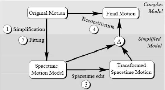
However, the complexity of human musculoskeletal structure often leads the optimization problem to convergence difficulties. Zoran Popovic et al addressed this problem by mapping the original character structure to a simplified model with drastically reduced degrees of freedom (DOFs). Their entire algorithm breaks down to four stages.
Figure 2: Algorithm outline of motion transformation
First, character simplification creates an abstract character model containing the minimal number of DOFs necessary to capture the essence of the input motion. Second, find the solution of spacetime optimization that matches the motion of simplified character model at fitting stage. Third, adjust spacetime motion parameters, kinematics and dynamics constraints, or even objective function to edit the resulting motion. Finally, remap the editing change in motion onto the original motion to produce the final animation.
8
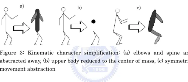
Fused body parts have redundant DOFs and the subtree of character hierarchy can be replaced with a single node in some cases of high-energy motion. By manually removing them, the simplified model not only captures the essence of the input motion without losing fundamental dynamics properties, but improves performance and facilitates convergence of the spacetime optimization.
Figure 3: Kinematic character simplification: (a) elbows and spine are abstracted away, (b) upper body reduced to the center of mass, (c) symmetric movement abstraction
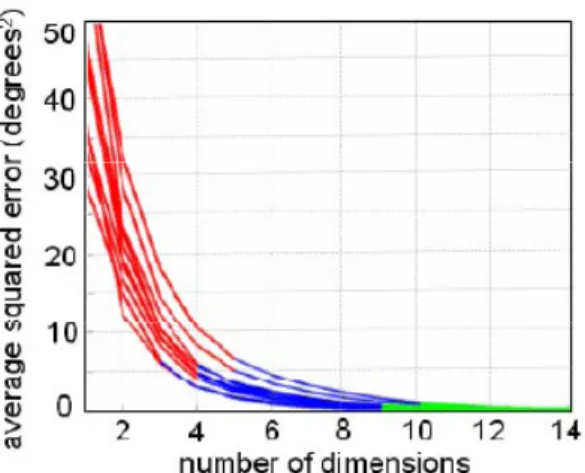
Instead of simplifying character model directly, Safonova et al [7] performed PCA to reduce the dimension of motion and solved spacetime optimization in a low-dimensional space. They exploited the observation of dynamic human motion having high degree of coordination. There is spatial coherence between body parts so that reduction of dimensionality is possible. For the common human behaviors, they found that five to ten dimensions are sufficient.
9
Figure 4: Error between a full-dimensional motion and the corresponding k-dimensional representation
In their implementation, PCA were used to find basis vectors from a set of example motions. They solved the optimization problem to obtain the coefficients of linear combination of basis vectors that form the desired motion. Constraints were specified in the full-dimensional space and then projected onto the low-dimensional space. As long as the choice of example motion capture clips is similar behaviors to the desired motion, spacetime optimization in this approach can work well and effectively to generate natural-looking character animation.
Liu et al [3] proposed another approach that does not reduce the number of DOFs directly to improve spacetime optimization, but enforce linear and angular momentum of the motion to avoid heavy computation of complex dynamical model. They kept the pattern of linear and angular momentum as dynamics constraints by invariants and splines respectively.
10
Figure 5: The general angular and linear momentum pattern of a jumping motion
Furthermore, Liu et al [4] introduced more sophisticated dynamical model that incorporates several factors of locomotion derived from the biomechanical literature. This model accounts for passive joint forces due to muscles, tendons and ligaments, and simulated by springs and dampers. In order to overcome the difficulties of fine tuning of these physical parameters, they proposed a new algorithm, Nonlinear Inverse Optimization (NIO) to estimate the values from motion capture data. The underlying paradigm of NIO is a spacetime optimization problem that assumes the captured motion is optimal and then solves unknown parameters inversely. After that the user can adjust these parameters to generate new animations.
In contrast to long-horizon optimal plans, da Silva et al [6] proposed a short-term approach. They presented a controller, McSim, composed of a predictive component and a low gain proportional-derivative (PD) component. The predictive component is a quadratic program (QP) with the linear dynamics model as constraints. It solves for the joint and external forces
11
which track the input motion for a short window of time into the future. Then the PD component compensates for the errors generated by the predictive component due to high latency and modeling assumptions. McSim guides the simulated character dynamics toward input motion data at interactive rates while sacrifices optimality for computational performance.
12
3 Methods
Our system first reads the human motion from a BVH file. BVH is a common file format used to store human motion. It arranges the articulation of human body in a hierarchy structure and specifies the motion data of each joint by three consecutive Euler angles, that is, rotation angle about Z axis, rotation angle about X axis and rotation angle about Y axis. Thus, there are 3 DOFs to describe a joint every frame.
Figure 7: Skeleton of human body
The above structure of human body has 18 joints. For a 5-second motion clip containing 165 frames, there are totally 8910 DOFs in this clip. If we treat each DOF as a variable in the optimization phase, such huge number of variables would result in a considerable computation time (even though this solution may not be an “optimial” solution because of local minimums) or a divergence situation. However, by utilizing spatial coherence and temporal coherence of human motion, we do not need to take all DOFs as variables in the optimization phase. In the following sections, details about how we reduce the number of variables would be introduced.
13
3.1 Segmentation
A human body has four limbs and a torso. Joints in the same part are more related than those in different parts because of the hierarchy structure. For example, the movement of right shoulder would affect the moving of right wrist, whereas there is no direct relationship between right shoulder and left wrist. Thus we divide limbs and the torso into different segments in order to maximize this kind of local spatial coherence. Moreover, keeping local spatial coherence also provides more flexible controbility.
Figure 8: Each color for a segment
There are 5 segments. Each segment is divided empirically according to the physical structure of human body. They are the Torso, RightArm, LeftArm, RightLeg and LeftLeg respectively.
z Torso: there are 4 joints, including Hips, Chest, Neck and Head.
z RightArm: there are 4 joints, including RightCollar, RightShoulder, RightElbow and RightWrist.
z LeftArm: there are 4 joints, including LeftCollar, LeftShoulder, LeftElbow and LeftWrist.
z RightLeg: there are 3 jonts, including RightHip, RightKnee and RightAnkle.
z Afte DOF
3.2
B optim keyf moti func syst z Figu cons LeftLeg: t er segmen Fs reductioKinem
By spec mization c frames int ion withou ction. The em: Position C The user specifying ure 9: (le straint there are 3 ntation, w on, whichatics Co
cifying a can provid terpolation ut discont ere are 3 Constraint can chang g this kind eft) Origin 3 joints, in e perform will be deonstrain
appropriat de compre n, the op tinuity de kinds of ts of End E ge the pos d of constr nal motio 14 ncluding L m PCA on escribed innts
te kinem hensive co ptimization efects by t kinemati Effectors sitions of e raints. on, (right) LeftHip, Le n each seg n section 3. matics c ontrol ove n process the smoot ics constr end effecto ) adjusted eftKnee an gment res .5. constraints r the moti iterativel th term in aints sup ors at cert d motion nd LeftAnk spectively. s, space ion. Instea ly adjusts n its obje pported in tain frame satisfied kle. For etime ad of s the ctive n our es by thez Figu cons z Environm The user the origin ure 10: (l straint Body Part By assum part is mo original m center of preserve physics pl ment Obsta can put s nal motion left) Origi ts Lengths ming unifo odulated p motion to mass (CO the balan lausible. acles Cons some boxli n is modifie inal motio s Constrai rm mass proportion a differe OM) const nce of hum 15 straints ike obstac ed to react on, (right ints denisty of nal to its le ent size of traints. Li man body cles in the t the condi t) adjuste f human b ength. So t f model b imiting th and make e environm itions surr d motion body, the m the user ca by combin he position e sure the ment such rounded it satisfied mass of a an retarge ing additi n of COM e motion t that t. d the body et the ional M can to be
Figu cons
ure 11: (l straint
left) Origiinal motio
16
17
3.3 Equilibrium-based Force Response
Instead of embedding complex dynamics to simulate human’s musculoskeletal model, we propose using the assumption of static equilibrium at each frame. This assumption take advantage of spacetime optimization such that we can only focus on the statics of each frame independently and let spacetime optimization keep the temporal connectivity between frames for us. In addition, by assembling 3 springs at X-axis, Y-axis and Z-axis respectively in the local coordinates for each joint, we do not need to induct novel variables as extra physics parameters in the optimization phase. To simulate the muscle force of some joint, we simply apply Hooke’s law for each spring of the joint.
Figure 12: A spring and a damper assembled at the joint
For some frame, the muscle force exterted by the joint i is made up of 3 component forces applied on local axes of the joint.
⎥
⎥
⎥
⎦
⎤
⎢
⎢
⎢
⎣
⎡
Δ
Δ
Δ
=
⎥
⎥
⎥
⎦
⎤
⎢
⎢
⎢
⎣
⎡
=
i z i z i y i y i x i x i z i y i x ik
k
k
f
f
f
F
θ
θ
θ
, where i xθ
Δ
,Δ
θ
yi and i zθ
18
By assuming that the original posture of human body at each frame is in static equilibrium, we do not need to calculate muslce forces when there is no external force; otherwise, the net force of total muscle forces and the external force must equal to zero. An external force is an additional force specified by the user to apply on some joint. It is a vector including magnitude and direction of the external force. Once the external force being added into the system, the whole human body is no longer in the state of static equilibrium. As a result, angles of joints must be changed to exert muscle forces to counteract ths external force.
Every joint in the hierarchy would contribute 3 forces, each lying on the direction of its local axis. Then we transform these forces from their local coordinates to the world coordinates. Finally, all forces are projected onto the vector of the external force. Because the external force is set as a constraint, optimization process will drive the net force to zero.
G G External Force Figure 13: Equilibrium θi Joint i Fi = kiθi θj Fj = kjθj External Force Joint j Gj Gi
T syst z t f e c z m s f Figu cons There are em: Permanen This k the motion force. For external f constraint Instant F This k motion. B spline inte frame and ure 14: (le straint app e 2 kinds o nt Force C kind of con n in the w example, force whic t. Force Cons kind of co ecause we erpolation d its neigh ft) Origina plied to th of force co Constraint nstraint is whole anim we can inc ch points t traint onstraint i e treat eac n is used t tbor frame al motion, he left limb 19 onstraints s applied t mation wi crease the to negativ is only ap ch frame to hold the es. , (right) ad b of body that the to the ent ill be influ e weight of ve Y-axis pplied to as an ind e connecti djusted m user can ire motion uenced by f right arm as the pe a specific dependent ivity betw motion sati specify in n clip. Tha y this exte m by addin rmanent frame in static sys een the ta isfied the n our at is, ernal ng an force n the stem, arget force
20
3.4 Spacetime Optimization
The kernel of our system is a sequential quadratic programming (SQP) problem. We define the objective function companied with kinematics constraints and force constraints, and then solve our problem by the SQP solver SNOPT.
Such a motion optimization process is based on the original motion to ensure reality and also try to fit all user-specified constraints for motion editing. Thus the objective function is designed to preserve both smooth of the motion and similarity between the original motion and the result motion.
(
)
(
)
[
]
∑∑
− = − = −Θ
−
−
+
−
=
2 1 1 0 2 2 1(
1
)
n i m j j i j i j i j i j objf
ω
α
θ
θ
α
θ
, whereω
j: the weight of DOF j,
∑
− =
=
1 01
m j jω
α
: the weight of continuity,0
≤
α
≤
1
j i
θ
: DOF j at i ’th frame of the motionj i
Θ
: DOF j at i ’th of the original motionThe superscript j indicates the index of joint, and the subscript i
indecates the index of frame. As a result, the first term in the above equation means that DOFs of the same joint between 2 consecutive frames should be close, while the second term means that the DOFs of joints in the target and original motion should be close as well.
21
In order to maximize accuracy and efficiency of the SQP solver, we provide the gradient of each DOF as follows,
(
) (
) (
) (
)
[
]
(
) (
) (
)
[
]
(
j)
i j i j i j i j j i j i j i j i j i j i j j i j i j i j i j i j i j i j i j i j j i objf
Θ
−
−
−
=
−
−
Θ
−
+
−
=
∂
Θ
−
+
−
+
Θ
−
+
−
∂
=
∂
∂
+ − + − + + + − 1 1 1 1 2 1 1 2 1 2 2 13
2
2
2
2
θ
θ
θ
ω
θ
θ
θ
θ
θ
ω
θ
θ
θ
θ
θ
θ
θ
ω
θ
With sufficient information of gradients, computation time the SQP solver spending on finding out solutions can be reduced about 100 times. The number of iterations can also be decresed greatly to reach acceptable accurate results.
For all constraints, we append them to the objective function as soft constraints rather than hard constraints. The objective function becomes
(
)
(
)
[
]
C
f
c n i m j j i j i j i j i j c obj=
−
ω
∑∑
ω
α
θ
−
θ
+
−
α
θ
−
Θ
+
ω
− = − = − 2 1 1 0 2 2 1(
1
)
)
1
(
, where wc is the weight of constraint. It is a trade-off between accuracy and
efficiency. We observed that little loss of accuracy can gain great time spent on trivial computation. At last, we refine the inaccuracy with Inverse Kinematics (IK).
22
3.5 Principle Components Analysis
To further improve the efficiency of spacetime optimization, we propose to use PCA to reduce the number of DOFs. Because PCA can preserve the most significant features or styles of data sets during transformation, in the situation of motion data it captures the major movement of body. When considering the hierarchy of human structure, the movings of joints which belong to the same body part are most correlated. Consequently, we perform PCA on each body segment independently such that less number of principle components can hold more accordant information without the bothering of unrelated data.
We arrange frame data as a n m matrix, where n is the number of original DOFs and m is the number of frames. After applying PCA, we can get the matrix of eigenvectors stored in column-major and the matrix of deviations as follows:
X VB Z
X: original data matrix, n by m V: matrix of eigenvectors, n by n B: matrix of deviations, n by m Z: matrix of z-scores, n by m
Eigenvectors in V are sorted according to their cumulative energy such that the eigenvector with the largest-magnitude eigenvalue is at the left.
23
energy. It results in a submatrix W of V and a submatrix Y of B. The dimension of W is n n, where n is less than n, and the dimension of Y is n m. Finally, we use the elements of Y as the variables in optimization process instead of the original DOFs. In practice, n is usually half of n by preserving 98% energy because there is high coherence among joints in the same body segement.
At optimization, the object function is bascally uncanged except that variables are not original DOFs any more, the elements of sub deviations matrix Y instead. Then the gradient of each variable is slightly modified as follows:
(
)
∑
⎥
⎥
⎦
⎤
⎢
⎢
⎣
⎡
∂
∂
Θ
−
−
−
=
∂
∂
+ −x
x
f
j ij i j i j i j i j objω
θ
θ
θ
θ
1 13
2
, where summation means that all joints of the hierarchy described by the eigenvector related to x.
3.6 Spline Interpolation
To exploit temporal coherence between consecutive frames and further improve the quality of synthesis results, we use optimized key frames as control points of splines. Key frames are selected at regular intervals from the original motion. After applying PCA to their DOFs, the elements left in the matrix of deviations are set as variables in optimization process. To reconstruct the whole result motion, we simply interpolate other frames from these key frames.
24
4 Experiments and Results
There are 3 kinds of parameters that need to adjust manually. They are weight of continuity, weights of joints and force constants of joints, respectively.
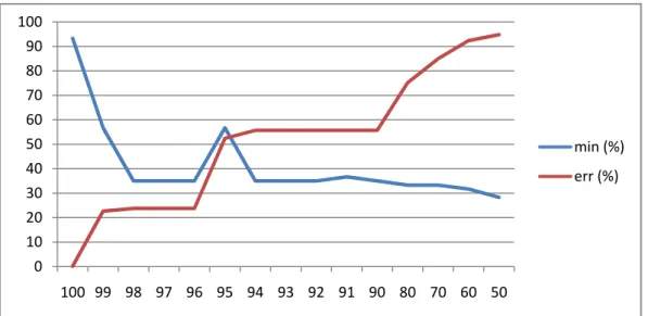
4.1 Weight of Continuity
Weight of continuity influences the continuity between frames. The more weight of continuity, the more smooth of the motion. However, the constraints may not be satisfied accurately when keeping smooth. It results in a trade-off between smooth and accuracy. In practice, weight of continuity can be set heigher for environment obstacle constraints than for constraints of end effectors. Because the end effector does not need to hit a target precisely in the case of environment obstacle constraints, high weight of continuity can help the synthesis result look like more gracefully.
Figure 15: Relationshiop between accuracy and computation time
In Figure 15, it shows more computation time needed for higher
0 10 20 30 40 50 60 70 80 90 100 100 99 98 97 96 95 94 93 92 91 90 80 70 60 50 min (%) err (%)
accu Com minu seco para uracyframe mpared wit utes for 90 onds to c ameters. Length QP Solver CPU Figur es. The t th 100% ac 0% to 98% complete 32 fram r Conjug Interl C 100 : 0 80 : 20 re 16: Accu ime is re ccuracy, th % accuracy with oth mes gate-gradie Core 2 670 uracy betw 25 epresented he computa y. In pract her minor ent 00 @ 2.66 G Table 1 99 : 1 70 : 30 ween differ d by the ation time tice, a 32-f r modific Tim Iter GHz Mem rent weigh precentag e is reduce frame clip ations of me ≒ ations 30 mory 3. 90 : 10 60 : 40 hts of conti ge of minu ed greatly t takes abo f optimiza ≒6 seconds 00 .25 GB inuity utes. to 35% out 6 ation s
26
4.2 Weights of Joints
Joint Weight Joint Weight Hips 4000 RightKnee 100 LeftHip 1000 RightAnkle 10 LeftKnee 100 Chest 2000 LeftAnkle 10 LeftCollar 1000 RightHip 1000 LeftShoulder 100 LeftElbow 10 RightElbow 10 LeftWrist 1 RightWrist 1 RightCollar 1000 Neck 10 RightShoulder 100 Head 1 Table 2
4.3 Force Constants of Joints
Joint Value of k Chest 4 Collar 8 Shoulder 8 Elbow 4 Wrist 2 Table 3
4.4 Results
z Original Motion28
29
z Force Constraint
31
5 Conclusions and Future Works
This thesis proposes a spacetime optimization based motion editing system which solves the configuration of joints satisfying user-specified kinematics and forces constraints. We exploit spatial and temporal coherence of human motion to save computation time while providing various kinds of constraints. With appropreiate set of kinematic constraints, QP solver can find acceptable solutions without tracking accurate muslce forces by a complex musculoskeletal model. To further expand the limits of kinematic constraints, we propose equilibrium-based force response model to efficiently counteract external forces or joint weight modifications.
However, the values of manual parameters such as weights and force constants play an important role to the synthesis results. One of our system limits is that the user needs to tune these parameters for the best results. In contrast to physics-based spacetime optimization approach, there are only 3 kinds of weights needed to tune manually in our system. It does not spend time on extracting massive physical parameters, neither. As a result, the performance can reach 6 times of real-time at best cases.
In the future, the most important work is to incorporate balance maintenance mechanism into our system, such as considering feedback forces in the supporting phase. Besides, gradient calculations in the optimization process can be further programmed generalized so that more kinds of kinematic constraints can be included with a friendly user interface. Furthermore, the QP solver can be re-implemented to a parallel environment to enhance the performance.
32
6 References
[1] WITKIN, A., AND KASS, M. “Spacetime constraints.” Proceedings of Siggraph. (1988)
[2] POPOVIC, Z., AND WITKIN, A. “Physically based motion transformation.” Proceedings of Siggraph. (1999)
[3] SAFONOVA, A., HODGINS, J. K. AND POLLARD, N. S. “Physically realistic human motion in low-dimensional, behavior-specific spaces.” Proceedings of Siggraph. (2004)
[4] LIU, C. K., AND POPOVIC, Z. "Synthesis of Complex Dynamic Character Motion from Simple Animations." Transactions on Graphics. (2002)
[5] LIU, C. K., HERTZMANN, A. AND POPOVIC, Z. “Learning physics-based motion style with nonlinear inverse optimization.” Proceedings of Siggraph. (2005) [6] DA SILVA, M., ABE, Y. AND POPOVIC, J. “Simulation of Human Motion Data
using Short-Horizon Model-Predictive Control.” Eurographics. (2008)
[7] DA SILVA, M., ABE, Y. AND POPOVIC, J. “Interactive Simulation of Stylized Human Locomotion.” Proceedings of Siggraph. (2008)
[8] BARBIC, J., SAFONOVA, A., PAN, J. Y., FALOUTSOS, C. AND HODGINS, J. K. “Segmenting Motion Capture Data into Distinct Behaviors.” Graphics Interface. (2004)
[9] GLEICHER, M. "Motion editing with spacetime constraints." Proceedings of Symposium on Interactive 3D Graphics. (1997)
[10] PULLEN, K., AND BREGLER C. “Motion capture assisted animation: Texturing and synthesis.” Proceedings of Siggraph. (2002)
33
[11] TAK, S. AND KO, H. “A physically-based motion retargeting filter.” Transactions on Graphics. (2005)
[12] AMIROUCHE, F. Fundamentals of Multibody Dynamics. Birkhauser, 2004. FEATHERSTONE, R. Robot Dynamics Algorithms. Kluwer, 1987