Dynamic Average Method for Cycle Time Estimator in an IC Fab
Han-Pang Huang *, Chien-Fa Yeh
*,
Jia-Yang Juang*,
Li-RenLm
**,
Thomas Chen**
Robotics Laboratory, Department of Mechanical Engineering National Taiwan University, Taipei, TAIWAN 10674, R.O.C.
e-mail: hphuang@w3.me.ntu.edu.tw
TELFAX: (886)2-23633875
*Professor and correspondence addressee *Graduate student **Fab 3 Manufacturing Dept.
,
Taiwan Semiconductor Manufacturing Co. Ltd.ABSTRACT
The forecast of process cycle time is difficult in an IC manufacturing system, especially in an environment with multiple products and various processes. In this paper, a simple forecast mechanism is developed to provide the forecast of product’s cycle time and product’s remaining process cycle time, and other useful processing information. The proposed algorithm is based on a dynamic average of historical process data stored in database to generate run- time, wait-time and hold-time information, and the results are further classified in terms of tool group (or tool), technology and stage-id hierarchically. The product’s remaining process cycle time can be obtained by looking for the product’s state from on-line data in database first, and then utilizing product’s operation flow table and the average process time given above to calculate it. For calculating product’s cycle time, it works in a similar way. Since the run-time, wait-time and hold-time of each lot can be shown from the proposed algorithm, it is easy to forecast the operation bottleneck of the lot. This method is proved to be useful by testing in Fab 3 of TSMC (Taiwan Semiconductor Manufacturing Company).
Key words: Process cycle time forecast, bottleneck forecast
INTRODUCTION
The modem semiconductor foundry business has become more competitive. In order to sustain superiority, the total satisfaction of customers is getting more and more important. To achieve 100% on-time delivery and reduce cycle time of products are two of the most challenging tasks for the IC fab. Since Fab 3 of TSMC is a purely foundry fab, the necessity of improving service level of on-time delivery to customers arises. Accordingly, a system utilized to promote the performance of on-time delivery is necessary. However, the manufacturing process of semiconductor devices is highly complex, nonlinear, expensive and re-entrant [6,9,13]. The
re-entrant phenomenon is very typical in a IC fab. Namely, as wafers move from one step to another, they often return to a given tool. A €ab consists of several hundred tools grouped into dozens of distinct tool groups. It is very difficult work
for engineers to construct such a system described above. In literature, several algorithms [ 1- 1 1, 13- 151 are proposed for cycle time estimation.
Ehteshami and et al. [3] commited to delivery dates for a product by using historical average cycle time and adding some safety margin. He designed the margin to compensate for variability in the cycle time and to meet the desired service level. This is one kind of well-known SLACK policy. Several issues based on SLACK policy had also been addressed in [2,5,7]. Adl and et al. [l] proposed hierarchical modeling and control technique. A low-level tracking policy was presented and integrated with a high-level state variable feedback policy. The low-level tracking policy was to track low-frequency commands generated by the high-level controller. Such issues had also been addressed in [4,9,11,13,14]. Raddon and et al. [SI developed a model for forecasting throughput time. Another approach which has been addressed by many other researchers is flow model [6, 11,14,15]. Flow models prehct the fab’s behavior over a long-time scale. Sattler [lo] used queueing curve approximation in a fab to determine productivity improvements.
In this paper, we construct a simple cycle time estimator, with least programming effort, whch can forecast products’ cycle time, remaining cycle time, and other useful processing information, such as work-in-process (WIP) and bottleneck of the operation flow. Dynamic average method for cycle time estimator is proved to be useful by testing in Fab3 of TSMC. More detailed description will be introduced in the subsequent sections.
ESTIMATOR FORMULATION AND ANALYSIS
The main concept of dynamic average method can be divided into four steps described as follows:
Stepl: Look for three or four key parameters having the most significant effect on cycle time which are determined heuristically. The attributes selected are tool group (or tool), technology and stage-id. Step2: Construct a cycle time estimator based on dynamic
average method. It dynamically averages historical process data in a fab to generate run-time, wait- time and hold-time information, which are classified in terms of tool group (or tool), technology and stage-id hierarchically. The results are kept as references.
Step3: Look for the interested lot’s state f?om on-line data in database. Utilize lot’s operation flow table as
well as the reference table obtained in Step2 for each step. Therefore, the estimation of each step- time defined as the sum of processing time and waiting time through a tool can be obtained. As a result, the remaining cycle time of the lot is forecasted.
Step4: Adjust the priority of lots by comparing the difference of the forecasted due date and commit due date.
A high-volume modern fab consists of abundant tools grouped into dozens of tool groups. Collections of wafers, known as lots, move from one tool group to another undergoing hundreds of steps (or operations) before completion. Each lot follows a fabrication procedure that corresponds to the product family to whch the lot belongs. The fabrication procedure of a particular product IC is kept in a process log (or an operation flow table). The log completely records the all parameters of each step including relative tool group, recipe, stage-id and other process information. Typically, each product family contains 200 to 300 or even more process steps. Thousands of lots belonging to different products are circulating in the fab at any given time.
Since step-time is composed of processing time and waiting time, it is reasonable to consider them individually. For an IC fab, there are many parameters that affect both the processing time and waiting time of lots. They are listed in Table 1.
Table 1. Associated parameters list
priority of lots, quantity of lots in fab, the
In order to simplify the problem, we attempt to look for three or four key parameters having the most significant effect on step-time. These key parameters are determined heuristically through analysis of the physical meaning by experienced engineers. The attributes selected are tool group (or tool), technology and stage-id. Technology of a product represents its product type, such as memory or logic, and technology level, such as .35 or .30. A stage-id is a collection of steps which have similar process, such as Wafer-start stage, Plug-etchback stage, Wafer-out, etc.
Tool, technology, stage-id are the common parameters
affecting both processing time and waiting time. There are several hundreds of tools in a fab. The processing time of a tool is dramatically different from one to another. For example, the time spent on some processes, such as difTision and LPCVD, may be up to several hours. On the contrary, the time spent on wet etchmg is only several minutes. The reason of choosing stage-id as one of key parameters is similar. The dwersity of semiconductor products causes the variation of step-time. For example, the time spent on .30 process is longer than
S O
process. It is reasonable to choose technology as another key parameter.After the key parameters are determined, we construct a cycle time estimator based on the average method. It averages historical process data stored in database in the fab to generate run-time, wait-time and hold-time information classified by tool group (or tool), technology and stage-id hierarchically. It is shown in Figure 1.
TECH 1
A,
:
1:
r=::z:
STAGE TIME STAGE TIME TOOLG 1 (TOOL) TECH n STAGE STAGEFigure 1. The estimator averages historical process data stored in database in a fab to generate run-time, wait-time and hold-time information classified by tool group (or tool), technology and stage-id hierarchically.
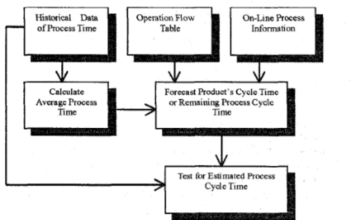
The architecture of dynamic cycle time estimator is shown
in Figure 2.
Historical Data On-Line Process
of Process Time
Figure 2. The archtecture of dynamic cycle time estimator The data flow is described as follows:
The associated historical data of lots including start time of steps, end time of steps, technology, stage-id, tool group, recipe, priority and other parameters are available in the fab. First, the data in the database is used to calculate the several-
day averages of run-time, wait-time and hold-time classified by tool group (or tool), technology and stage-id hierarchically. The result is kept as a reference table. Second, we look for the interested lot's state from on-line data in database. From the operation flow table, information of each step can be obtqined including which combination of tool group, technology and stage-id the step belongs to. By referring each step to the reference table, the forecasted step- time is acquired. By summing each step-time of the residual steps of the lot, the remaining cycle time of the lot is forecasted. The reference look-up table is updated everyday to dynamically track the change of on-line data.
The estimator provides a preliminary forecast. In order to achieve on-time delivery, Fab3 uses the Least Slack policy as a scheduling policy [5,7] accompanied with cycle time estimator. Suppose each lot i arriving to the fab with a due date denoted as 6(i). The estimated remaining cycle time of lot i at time t obtained by the estimator is denoted as
r
i(t), i.e.,[ i(t) :=estimated remaining cycle time of lot i at time t (1)
The quantity 6 (i)
-
t-
i(t) denotes the relative urgency of lot i. However, if an idle tool has to decide which of the two lots it should serve next, it is reasonable to select the lot i which 6 (i)-
t-
[ i(t) is the smallest; i.e., the most urgent lot. Fab3 defines the slack s(i) of a lot ias
s(i):= 6 (i)
-
t-
C
i(t) (2)The slack s(i) can tell how much time a lot has been ahead or behmd its commit due date.
This
has been found helpful in communication with the management and training of operators. As the degree of urgency is determined, on-time delivery performance can be improved by adjusting the priority of lots. All lots in Fab3 are classified into 5 priority classes. They are super hot run (SH), hot run (H), rush (R), normal (N) and slow (S). The SH lots have the highest priority to be served, while the S lots have the lowest priority. All lots belong to these five classes.FORECASTING RESULTS
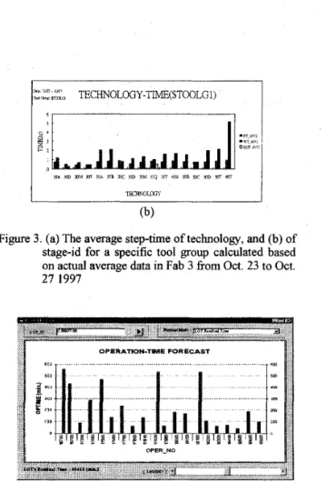
The average step-time of stage-id and technology for a specific tool group is calculated based on actual data in Fab 3 from Oct. 23 to Oct. 27 1997. It is shown in Figure 3. The forecasted lot's remaining cycle time for a specific lot is shown in Figure 4. The x-axis is operation number of the lot. Each step-time and remaining cycle time can be read easily.
D . l r l O l - l - l o l .
T'd o w I T D M STAGE-l"E($IWXl)
h e >om Im
moiblloaG, TECHNOLOGY-TIME($TOOLGl)
6 , I
Figure 3. (a) The average step-time of technology, and (b) of stage-id for a specific tool group calculated based on actual average data in Fab 3 from Oct. 23 to Oct. 27 1997
OPERATION-TIME FORECAST
Figure 4. Forecasted lot's remaining cycle time. The x-axis
is operation number of the lot.
The error of estimated remaining cycle time of 53 lots of a specific product is shown in Figure 5. The average error is about 1 1.5%.
No. of Data
- A.:,.cnx - FC51.CTUF
Figure 5. The error of estimated remaining cycle time of 53 lots of a specific product in Fab3
Generally speaking, the error of the forecasted cycle time is under 20%.
CONCLUSION
can improve the on-time-delivery perfomance of a fab with least programming efforts has been addressed in this paper. The main feature is its simplicity and easy to understand. It is proved to be useful by testing in Fab3. In addition, the forecasted result is more precise than the original Turn Ratio method. The existent Least Slack policy needs a precise remaining cycle time estimator, then the correct urgency of each lot can be obtained. As the remaining cycle time of lots are forecasted, the Least Slack policy can be applied to improve the mean and variance of cycle time.
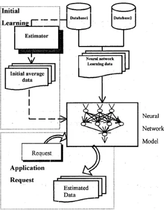
In the future, the estimated data can promde an mitial reference for the on-line learnmg system such as neural network learning system. The architecture is shown in Figure 6
Neural Network Model
.. ... . . .... ... ... .... . .... ... . .. . ... . ... . . ... .. ...
Figure 6. Estimated data can provide an initial reference for other on-line learning system such as neural network learning system.
REFERENCES
[l] M. K. Adl, A. A. Rodriguez, K. S. Tsakalis,
“ Hierarchical Modeling and Control of Re-entrant
Semiconductor Manufacturing Facilities”. Proceedmgs of the 35th Conference on Decision and Control Kobe, Japan, 1996.
[2] R. W. Conway, et. al., “Theory of Scheduling,” Readmg, MA: Addison-Wesley, 1967.
[3] B. Ehteshami, et. al., “Trade-off in Cycle Time Management: Hot Lots,” IEEE Trans. Semicond. Manufact., Vo1.5, No.2, pp.101-106, 1992.
[4] S. Gershwin, “Manufacturing Systems Engineering”. Prentice Hall, Engelwood Clifs, 1994.
[5] C. H. Hung, C. M. Liu, T. Chen, “Managing on Time Delivery during Foundry Fab Production Ramp-up,” [6]
AP.
R. Kumar, “Re-Entrant Lines”. Technical report, Coordinated Systems Lab., University of Illinois, Urbana, IL, received 1994.[7] C. H. Lu, et. al., “Efficient Scheduling Policies to Reduce Mean and Variance of Cycle-Time in Semiconductor Manufacturing Plants,“ IEEE Trans. Semicond. Manufact., Vo1.7, No.3, pp.374-388, 1994.
[8] A. Raddon and B. Gngsby, “Throughput Time
Forecasting Model,” IEEEBEMI Advanced Semiconductor Manufacturing Conference, pp.430-433, 1997.
[9] A. A. Rodriguez and M. Kawski, “Modeling and Robust Control of Re-entrant Semiconductor fabrication Facilities: Design of Low-Level Decision policies”. A
Proposal to Intel Research Council, 1994.
[ 101 L. Sattler, “using Queueing Curvw Approximation in a Fab to Determine Productivity Improvements”. IEEEEEMI Advanced Semiconductor Manufacturing Conference. Texas Instruments, Inc. Dallas, TX, 1996 [ l l ] S. P. Sethi and Q. Zhang, “Hierarchical Decision
Making in Stochastic Manufacturing Systems”. Birkhauser 1994.
[12] M. Sugeno and
G.
T. Kang, “Structure Identification of Fuzzy Model,” Fuzzy Sets and Systems, vo1.28, pp. 15- 33, 1988.E131 K.
S .
Tsakalis, et. al., “Hierarchical Modeling and Control for Re-entrant Semiconductor Fabrication Lines: A Mini-Fab Benchmark,” IEEEBEMI Advanced Semiconductor Manufacturing Conference, pp.508-5 13,1997.
E141 K. Tsakalis, “Notes on Modeling of Re-entrant Systems”. Unpublished notes, Arizona State University,
1994.
[ 151 R. Alvarez-Vrgas, Y. Dallery and R. David, “ A study
of the Continuous Flow Model of Production Lines with Unreliable Machmes and Finite Buffers”. Journal of Manufacturing Systems, vol. 13, no. 3.
pp. 18-34.