探討不同纖維排列下複合材料之機械行為

國 立 交 通 大 學

機械工程學系

碩 士 論 文

探討不同纖維排列下複合材料

之機械行為

Investigating the mechanical behaviors of fiber composites with

different fiber arrays

研 究 生 ：齊揚楷

指導教授 ：蔡佳霖 博士

探討不同纖維排列下複合材料之機械行為

Investigating the mechanical behaviors of fiber composites with

different fiber arrays

研 究 生：齊揚楷 Student：Yang-Kai Chi

指導教授：蔡佳霖 Advisor：Jia-Lin Tsai

國 立 交 通 大 學

機 械 工 程 系

碩 士 論 文

A Thesis

Submitted to Department of Mechanical Engineering College of Engineering National Chiao Tung University

in partial Fulfillment of the Requirements for the Degree of

Master in

Mechanical Engineering

July 2007

Hsinchu, Taiwan, Republic of China

探討不同纖維排列下複合材料之機械行為

學生：齊揚楷 指導教授：蔡佳霖

國立交通大學機械工程學系碩士班

摘 要

本研究目的在於探討纖維複合材料在不同纖維排列情況下對其

機械性質之影響，而主要探討的幾何排列分為下列三種，正方型排列

(SEP)，對角線排列(SDP)，六角形排列(HP)。本論文將對此三種不同

排列之纖維複合材料做以下探討，熱殘留應力對於不同纖維排列之複

合材料其非線性機械行為之影響，以及不同纖維排列下複合材料之阻

尼 響 應 。 在 模 擬 纖 維 複 合 材 料 時 ， 將 取 出 一 代 表 性 單 元 體

（Representative Volume Element, RVE）進行分析，進而推求出整體

纖維複合材料之機械性質。在材料特性方面，纖維部份假設為線彈性

且具低阻尼特性，而基材部份則假設為非線性且具高阻尼特性。在熱

殘留應力對機械性質之非線性影響的分析裡，利用

Paley 以及 Aboudi

[1]所 提 出 的 微 觀 力 學 廣 義 網 格 法 (Generalized Method of Cells,

GMC)，來做纖維以及基材的熱殘留應力分析。再經由數值上的運算，

建構出含有熱殘留應力之纖維複合材料的應力應變關係。分析結果顯

示，相較於對角線纖維排列，熱殘留應力對六角形及正方型纖維排列

之機械性質之影響，來的輕微了許多。

對於不同纖維排列之複合材料對其阻尼影響的分析中，於代表性

單元體上分別施以相對於材料主軸方向的單軸載重或是剪力，利用微

觀力學廣義網格法，推求纖維複合材料主軸方向的應變能及其相對應

的應變能消散量。藉由應變能消散概念，計算出纖維複合材料位於各

材料主軸方向上的阻尼參數。從有限單元的分析方法，首先求出纖維

複合材料所構成的桿或平板結構，分別在自由邊界 (free-free) 以及一

端固定 (clamp-free)的情況下，其自由震動振動模態之變形﹔並結合

材料主軸方向上之阻尼係數以及振動模態之變形，即可求得在不同纖

維 幾 何 排 列 下 ， 對 於 不 同 結 構 的 模 態 振 動 阻 尼 效 應

(Damping

Capacity) 。由分析結果可觀察出，在由對角線排列所構成的桿或平

板之複合材料結構上，在前三個振動的模態中，所求得之阻尼效應，

分別大於另外兩種纖維排列。

Investigating the mechanical behaviors of fiber composites

with different fiber arrays

Student：Yang-Kai Chi 　 Advisor：Dr. Jia-Lin Tsai

Department of Mechanical Engineering

National Chiao Tung University

Abstract

This study aims to investigate the effect of fiber array on the mechanical responses of fiber composites. Basically three different fiber arrays, i.e., square edge packing (SEP), square diagonal packing (SDP), and hexagonal packing (HP), were considered in the analysis. The sensitivities of thermal residual stress on the nonlinear constitutive behaviors as well as the damping behaviors of the composites with different fiber arrays were the focus of the research. The representative volume element (RVE) containing fiber and matrix phase was employed to describe the overall mechanical behaviors of fiber composites. For the fiber phase, it was assumed to be a linear elastic material with low damping capacity, whereas the matrix was a nonlinear material with high damping capacity. The generalized method of cell (GMC) micromechanical model originally proposed by Paley and Aboudi [1] was extended to include the thermal-mechanical behavior, from which the thermal residual stress within the fiber and matrix phases was calculated. Through a numerical iteration, the constitutive relations of the composites in the presence of residual stress were established. Results show that for the composites with square edge packing,

the mechanical behaviors are affected appreciably by the thermal residual stress. On the other hand, the composites with hexagonal packing and square diagonal packing are relatively less sensitive to the thermal residual stress.

Regarding the damping behaviors of the composites, the RVE was subjected to a simple loading (either axial or pure-shear loading), and the corresponding damping properties of the fiber composites with respect to the material principal directions were calculated from the GMC analysis together with the energy dissipation concept. With the assistance of FEM analysis, the mode shapes of composite rod and plate structures with vibration under free and clamp boundary conditions were determined. In conjunction with the model shape and the damping properties, the damping capacity of the composite structures constructed based on unidirectional composites with different fiber arrays were calculated. It was found that, in both composite structures, the square diagonal packing always exhibits better damping performance rather than other two fiber arrangements at first three vibration modes.

誌謝 兩年的研究生活，看似很短不過這是我至今最努力也是最忙碌的兩年，此篇 論文最感謝指導教授 蔡佳霖博士，感謝他細心以及耐心的指導，並且幫我校正 許多論文上的缺失。同時也感謝清華大學動機械葉孟考教授、交通大學機械系蕭 國模教授撥空擔任學生口試委員，並且在口試的過程中給予保貴之意見，讓此篇 論文更佳完整。 感謝實驗室的全體同仁以及 245、247 有情有義的夥伴們，讓我有說有笑的 度過這的兩年，尤其是曾世華學長，對於課業以及研究給予我許多指導，此外我 也特別感謝已畢業的陳奎翰學長，謝謝他耐心的指導，讓我順利的銜接 GMC model. 最後謝謝我最敬愛的父母，有了你們的愛與關懷，讓我在求學的過程中，無 後顧之憂。

目 錄 中文摘要 ………... i 英文摘要 ………... iii 誌謝 ………... _v 目錄 _{………... vi} 表目錄 _{………... viii} 圖目錄 ………... _x Chapter 1 Introduction………... 1 1.1 Research motivation…..………... 1 1.2 Paper review………. 1 1.3 Research approach……… 4

Chapter 2 Effect of fiber array on thermal-mechanical behaviors of fiber composites... 6

2.1 Generalized method of cells (GMC) ……… 6

2.2 Nonlinear behavior of epoxy matrix………. 20

2.3 Thermal residual stress………. 23

2.4 Results and discussion………...………... 27

2.4.1 Convergence tests on the number of subcells……… 27

2.4.2 Influence of thermal residual stress on the behaviors of composites ………...………. 28

Chapter 3 Comparison of GMC, SCMC and FEM analysis………... 29

3.1 Strain compatible method of cells (SCMC)……….. 29

3.2.1 Boundary conditions and mesh….………. 34

3.3 Comparison of the results of GMC, SCMC and FEM analysis………… 37

Chapter 4 Effect of fiber array on damping behavior of fiber composites……… 39

4.1 Damping characterization using GMC……….………… 39

4.2 Calculation of vibration damping of composite structures………... 41

4.3 Discussions of the damping capacity of fiber composites with three different fiber arrays……. ………... 47

4.3.1 Vibration with free-free boundary condition………. 48

4.3.2 Vibration with clamp-free boundary condition………. 49

Chapter 5 Conclusions………... 51

References ………... 52

Appendix A MATLAB code for calculating the thermal residual stresses using GMC analysis……….. 54

Appendix B MATLAB code for GMC analysis………... 61

Appendix C MATLAB code for calculating the modal shapes and damping capacity of composite structures……….. 70

LIST OF TABLES

Table. 2.1 Mechanical properties and thermal properties of the ingredients of fiber composites used in the GMC analysis………. 79

Table. 3.1 Four parameters used in ANSYS to simulate the nonlinear behavior of matrix materials………... 80

Table. 4.1 Mechanical properties and damping capacities of fiber and matrix used in GMC analysis………. ……… 81

Table. 4.2 Damping property of fiber composites with SEP packing obtained by using the GMC and FEM analysis………. 81

Table. 4.3 Damping property of fiber composites with SDP packing obtained by using the GMC and FEM analysis………. 82

Table. 4.4 Damping property of fiber composites with HP packing obtained by using the GMC and FEM analysis………. 82

Table. 4.5 Fiber array effect on the first three modal damping capacities of composite rod with fiber extended in x-direction under free-free boundary condition…….………. 83

Table. 4.6 Fiber array effect on the first three modal damping capacities of composite rod with fiber extended in z-direction under free-free boundary condition……….. 83

Table. 4.7 Fiber array effect on the first three modal damping capacities of composite plate with fiber extended in x-direction under free-free boundary condition……….. 83

Table. 4.8 Fiber array effect on the first three modal damping capacities of composite rod with fiber extended in x-direction under clamp-free boundary condition……….. 84

Table. 4.9 Fiber array effect on the first three modal damping capacities of composite rod with fiber extended in z-direction under clamp-free boundary condition. 84

Table. 4.10 Fiber array effect on the first three modal damping capacities of composite plate with fiber extended in x-direction under one side clamped boundary condition……….. 84

Table. 4.11 Fiber array effect on the first three modal damping capacities of composite plate with fiber extended in z-direction under one side clamped boundary……….. 85

LIST OF FIGURES

Fig. 2.1 Representative volume element, (RVE)……….. 86

Fig. 2.2 Geometry and coordinate system of representative volume element………. 86

Fig. 2.3 Local coordinate systems of the representative volume element……… 87

Fig. 2.4 Fiber composites with three different fiber arrangements……….. 87

Fig. 2.5 RVE with square edge packing portioned into (a) 28

×

28 subcells and (b) 39

×

39 subcells………... 88

Fig. 2.6 RVE with square diagonal packing portioned into (a) 27

×

27 subcells and (b) 39

×

39 subcells…….……….. 88

Fig. 2.7 RVE with square edge packing portioned into (a) 20

×

35 subcells and (b)31

×

49 subcells………..………..……… 89

Fig. 2.8 Comparison of stress and strain curves obtained from the RVEs with coarse subclls and refined subcells……….………... 89

Fig. 2.9 Thermal residual stress effects on the stress and strain curves of 15° off-axis fiber composites with three different fiber arrays. (fiber volume fraction 60%)……… 90

Fig. 2.10 Thermal residual stress effects on the stress and strain curves of 30° off-axis fiber composites with three different fiber arrays. (fiber volume fraction 60%)……… 90

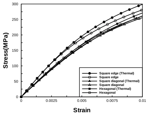
Fig. 2.11 Thermal residual stress effects on the stress and strain curves of 45° off-axis fiber composites with three different fiber arrays. (fiber volume fraction 60%)……… 91

Fig. 2.12 Thermal residual stress effects on the stress and strain curves of 60° off-axis fiber composites with three different fiber arrays. (fiber volume fraction 60%)……….………... 91

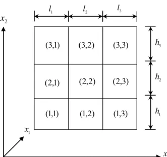
Fig. 3.1 Unit cell with 3

×

3 subcells to illustrate finite difference procedure……….. 92

Fig. 3.2 Coordinate system of the RVE with square edge packing fiber………. 92

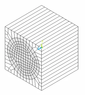
Fig. 3.3 Finite element mesh of the RVE with square edge packing fiber………... 93

Fig. 3.4 Finite element mesh of the RVE with square diagonal packing fiber………. 93

Fig. 3.5 Finite element mesh of the RVE with hexagonal packing fiber………. 94

Fig. 3.6 Finite element mesh for a quadrant of the RVE with square edge packing fiber………...……….. 94

Fig. 3.7 Finite element mesh for a quadrant of the RVE with square diagonal packing fiber………. 95

Fig. 3.8 Finite element mesh for a quadrant of the RVE with hexagonal packing fiber………. 95

Fig. 3.9 Coordinate system and dimension for a quadrant of the RVE with square edge packing fiber………... 96

Fig. 3.10 Stress strain curve of matrix employed in GMC, SCMC and FEM analysis………... ……… 96

Fig. 3.11 Comparison of stress and strain curves obtained from GMC and FEM analysis under transverse loading σ₂₂………. 97 Fig. 3.12 Comparison of stress and strain curves obtained from SCMC and FEM analysis under transverse loading σ₂₂……….. ……….. 97

Fig. 3.13 Converge test for the stress and strain curves of composites with hexagonal square edge packing fiber obtained from SCMC model under shear loading 12 σ ………... 98

Fig. 3.14 Converge test for the stress and strain curves of composites with hexagonal square edge packing fiber obtained from GMC model under shear loading

12

σ ………. ………. 98

Fig. 4.1 Modeling procedure for characterizing the damping properties of composite structures.……… 99

Fig. 4.2 The dimension of composite structures (a) composite rod with fiber extended in x-direction (b) composite plate with fiber extended in x direction………. 100

Fig. 4.3 The first three modal shapes of composite rod with fiber in x-direction under free-free boundary condition (a) First mode (b) Second mode (c) Third mode……… 101

Fig. 4.4 The first three modal shapes of composite rod with fiber in z-direction under free-free boundary condition (a) First mode (b) Second mode (c) Third mode……… 102

Fig. 4.5 The first three modal shapes of composite plate with fiber in x-direction under free-free boundary condition (a) First mode (b) Second mode (c) Third mode……… 103

Fig. 4.6 The first three modal shapes of composite rod with fiber in x-direction under clamp-free boundary condition (a) First mode (b) Second mode (c) Third mode……….………... 104

Fig. 4.7 The first three modal shapes of composite rod with fiber in z-direction under clamp-free boundary condition (a) First mode (b) Second mode (c) Third mode………...………. 105

Fig. 4.8 The first three modal shapes of composite plate with fiber in x-direction under one side clamped boundary condition (a) First mode (b) Second mode (c) Third mode……… 106

Fig. 4.9 The first three modal shapes of composite rod with fiber in z-direction under one side clamped boundary condition (a) First mode (b) Second mode (c) Third mode (SFM)……… 107

Chapter 1 Introduction 1.1 Research motivation

Fiber composites, because of their superior mechanical performances and light weight properties, have been extensively employed in various applications. This study aims to investigate the mechanical behaviors of fiber composites with three different fiber arrays, i.e., square edge packing, square diagonal packing, and hexagonal packing. The thermal-mechanical properties as well as the damping behaviors of composites are the focus in the paper. It is well known that the micro architecture of the fiber may influence the mechanical performance of the fiber composites. However, the extent of the fiber effect on the behavior of composites which are very crucial to composites design and application has not been studied systematically. In this paper, the micromechanical analytical scheme was employed to model the micromechanical structures of the fiber composites and the overall properties based on different microstructures were discussed.

1.2 Paper review

In the manufacturing process, the fiber composites were usually cured at high temperatures followed by the cooling stage to room temperature. During the cooling, because of the mismatch in the coefficients of thermal expansion of the fiber and matrix together with the mutual constraint effect, the thermal residual stress was induced in the constituents. The magnitude of the residual stress relies on the properties of the fiber and matrix as well as the associated microstructures of the fiber composites, including the fiber shape and fiber packing arrangements. In addition, the formation of residual stress may have influences on the constitutive behaviors of

the fiber composites, especially in the nonlinear range because the nonlinear behavior is highly dependent on the stress states of the composites.

The constitutive behaviors of the composites with different fiber architectures have been characterized by many researchers using either finite element analysis or analytical micromechanical approach [2–7]. Sun and Vaidya [2] use the finite element method to predict the elastic modulus for boron/aluminum by utilizing the periodic boundary conditions which was the salient of the representative volume element (RVE). Furthermore, Zhu and Sun [3] investigated the nonlinear behaviors of AS4/PEEK composites with three different fiber arrays under off-axis loading using finite element approach. It was found that the nonlinear behaviors of the composites were quite sensitive to the fiber packing arrangement. The similar conclusions were also addressed by Hsu et al. [4], who proposed an analytical micromechanical model for simulating the nonlinearity of AS4/PEEK composites subjected to combined transverse compression and shear loading. Orozco and Pindera [5] conducted a micromechanical analysis using the GMC model on the two-phase composites with randomly distributed fibers, indicating that as the number of the refined sub-cells in the unit cell is increased, the behaviors of the composites tend to be that of a transversely isotropic solid. The influences of fiber shape and fiber distribution on the elastic/plastic behavior of metal matrix composites were examined by Pindera and Bednarcyk [6] using the GMC micromechanical model. It was shown that the fiber packing exhibits a substantially greater effect on the responses of the composite materials than does the fiber shape. Pindera et al. [7] investigated the nonlinear behaviors of the boron/aluminum composites subjected to tensile, compressive and off-axis loadings. The thermal residual stress was considered in their analysis in order to explain the differences of initial yielding in tension and compression. The effect of residual stresses on yielding of SiC/Ti plates was also reported by Zhou et al.

[8]. Aghdam et al. [9] accounts for residual stresses, off-axis orientation and the interface condition between fiber and matrix on the constitutive behaviors of SiC/Ti metal matrix composites. However, their analysis is limited to single fiber array (square). A comprehensive review regarding the effect of fiber arrangement on the elastic and inelastic responses of fiber composites was provided by Arnold et al. [10]. In light of the aforementioned investigations, it was suggested that the behaviors of the fiber composites were mainly dominated by the fiber packing arrangements. However, few studies concerning the influence of the residual stress arising from curing associated with different fiber arrays on the performances of fiber composites have been reported.

Regarding to the damping behaviors of fiber composites, Saravanos and Chamis [11] used the unified micromechanical model to evaluate the damping property of unidirectional fiber composites with off-axis loading. Hwang and Gibson [12] utilized the finite element approach and the micromechanical strain energy to predict the damping property of the fiber-matrix interphase effects. It was also indicated that for the longitudinal, transverse and out of plane shear loading, material damping does not change much even though the interphase size was increased. In the previous review, most of the efforts were made to understand the basic damping properties of composites from the constitutive behavior of the ingredient in conjunction with the microstructure. However, the vibration damping responses of composite structures built based on the unidirectional composites with different fiber arrays has not been examined comprehensively so far. Although Kaliske and Rothert [13] utilized the GMC model to find the longitudinal damping property of fiber composites and then applied those damping properties to derive the structure modal damping capacity with the different fiber orientation, the microstructure effect on the damping responses was not discussed in their study.

1.3 Research approach

The outline of the thesis and the primary tasks of each chapter are addressed as follows. For the unidirectional composites, the fibers in general are displayed randomly within the matrix. To investigate the fiber array effect, three typical fiber arrangements, i.e., square edge packing, square diagonal packing, and hexagonal packing were assumed in our fiber composites. An appropriate RVE corresponding to each fiber array was selected in the micromechanical analysis where the fiber was considered to be linear elastic with low damping capacity, and the matrix was assumed to be a nonlinear with high damping capacity. By using Aboudi’s GMC micromechanical model [1], the incremental form of the constitutive relations of the composites was established in terms of the constituent properties as well as the geometry parameters of the RVE, from which the thermal residual stress within the ingredients was calculated. After a numerical iteration, the corresponding stress and strain relations of the composites in the presence of thermal residual stress subjected to off-axis loading were generated. The results were compared to those calculated from the composites without taking into account the thermal stress effect, which were presented in Chapter 2.

In addition, the fundamental assumptions in the GMC micromechanical model were examined and compared to the other micromechanical model. The stress and strain curves calculated based on the different micromechanical models were also discussed in Chapter 3.

Moreover, from the GMC micromechanical analysis, the stress-states within each ingredient can be evaluated properly. Based on the results, the damping capacity of the unidirectional composites with simple loading can be obtained using energy dissipation concept. With the damping capacity of the unidirectional

composites with different fiber arrays, the vibration damping properties of the composite structures can be calculated from the FEM analysis together with the energy dissipation concept. All detail procedures and results were illustrated in Chapter 4.

Chapter 2 Effect of fiber array on thermal-mechanical behaviors of fiber composites

In micromechanical analysis the constitutive behavior of fiber composites relies on the properties of fiber and matrix as well as the associated microstructure of fiber composites. In this chapter, the thermal-mechanical behaviors of composites with three different fiber arrangements will be compared. The generalized method of cells (GMC) proposed by Paley and Aboudi [1] was adopted for the micromechanical analysis in which the fiber is linear elastic and the matrix was treat as a nonlinear material. The organization of this chapter is outlined as following. The generalized method of cell was introduced to characterize the mechanical properties of the composites associated with their ingredient properties. Subsequently, the constitutive model was developed based on the plasticity theory for describing the nonlinear behaviors of matrix material. The thermal stresses generated in the fiber composites were calculated using GMC model and their effect on the nonlinear behavior of the composites were discussed.

2.1 Generalized method of cells (GMC)

In general, for the fiber composites, the fibers are arranged randomly in the matrix. In order to model the composites using micromechanical approach, we have to assume a certain fiber array within the matrix such that a representative volume element (RVE) (see Fig. 2.1) can be selected properly to describe the mechanical responses of the composites. In GMC analysis, the RVE was divided into several rectangular subcells (βγ) with β=1,....,Nβ and γ=1,...,Nγ. Depending on fiber

arrangement, each subcells indicates either fiber or matrix phase on the RVE. In Fig. 2.2, the area of subcell is equal to N_βl_γ and the fiber extends in the x1 direction.

Assume that a local coordinate system

(

( ) ( )γ

)

3 β 2 1 ,x ,x

x was located at the center of

each subcell and the displacement was assumed to be a linear expansion in terms of the distances from the center of subcell as

( ) _w( )

₍

_{x , x , x}

₎

_x( ) ( )_{φ x}( ) ( )_{ψ i 1,2,3} u βγ i γ 3 βγ i β 2 3 2 1 βγ i βγ

i = & + & + & =

& (2.1.1)

where is the displacement rates at the center of subcell. In addition, and are variables that characterize the linear dependence of displacement rates on the local coordinate system

( )βγ i w& ( )βγ i φ& ( )βγ i ψ& ) β ( 2 x , ( γ) 3

x . In elasticity, the small strain rate tensor is written as ( )

(

_u( ) _u( )

)

_{i,j 1,2,3} 2 1 η βγ i j βγ j i βγ ij = ∂ & +∂ & = (2.1.2) where ∂₁ =∂ ∂x₁, ( )β 2 2 =∂ ∂x ∂ and ( )γ 3 3 =∂ ∂x

∂ , substituting Eq. (2.1.1) into Eq.

(2.1.2) and using the average formula, we derived the average strain rates in any subcell (βγ) as ( )

_{∫ ∫}

( ) ( ) ( ) − − = l 2 2 l 2 h 2 h γ 3 β 2 βγ ij γ β βγ ij γ γ β β x d x d η l h 1 η (2.1.3)

( ) ( ) ( ) ( ) ( ) ( ) ( ) ( ) ( ) ( ) ( ) ( ) ( ) ( ) ( )βγ 2 1 βγ 1 βγ 12 βγ 3 1 βγ 1 βγ 13 βγ 2 βγ 3 βγ 23 βγ 3 βγ 33 βγ 2 βγ 22 βγ 1 1 βγ 11 w x φ η 2 w x ψ η 2 ψ φ η 2 ψ η φ η w x η & & & & & & & & & ∂ ∂ + = ∂ ∂ + = + = = = ∂ ∂ = (2.1.4)

It should be noted that the interface displacement rate of neighboring subcells and neighboring RVE must be continuous. This condition led to the following relation

( ) ( ) ( ) ( ) 2 h x γ βˆ i 2 h x βγ i βˆ βˆ 2 β β 2 u | | u_{& = = & =−} (2.1.5) _i( )βγ _x( ) _{l 2} ( )_iβγˆ _x( ) _{l 2} γˆ γˆ 3 γ γ 3 u | | u& ₌ = & ₌₋ (2.1.6)

where and are defined by βˆ γˆ

⎩ ⎨ ⎧ = < + = β β N β 1, N β 1, β βˆ (2.1.7) ⎩ ⎨ ⎧ = < + = γ γ N γ 1, N γ 1, γ γˆ (2.1.8)

( ) ( ) ( )

∫

( ) _{( )} ( )

∫

− = = − =− 2 l 2 l γ 3 2 h x γ βˆ i 2 l 2 l γ 3 2 h x βγ i γ γ βˆ βˆ 2 γ γ β β 2 hl u | dx 1 x d | u hl 1 & & (2.1.9)

Substitution of Eq. (2.1.1) into Eq. (2.1.9) yielded

( ) ( ) ( ) ( )βˆγ i βˆ γ βˆ i βγ i β βγ i h φ 2 1 w φ h 2 1

w& + & = & − & (2.1.10)

In the same manner, Eq. (2.1.6) was expressed as

( ) ( ) ( ) ( )βγˆ i γˆ γˆ β i βγ i γ βγ i l ψ 2 1 w ψ l 2 1

w& + & = & − & (2.1.11)

In Fig. 2.3, both Eq. (2.1.10) and Eq. (2.1.11) represent the displacement continuity in the interface between the subcells and all field quantities which are originated from the centerline ( )β of the subcell

2

x

( )

βγ and the centerline ( )βˆ 2

x of the subcell

( )

βˆγ . In order to introduce the location of the interface ( )I

2

x among subcells

(

βγ

)

and

( )

βˆγ , the centerlines were shifted as

( ) ( ) β I 2 β 2 h 2 1 x x = − (2.1.12) ( ) ( ) βˆ I 2 βˆ 2 h 2 1 x x = + (2.1.13)

Using a Taylor expansion of the field variables in Eq. (2.1.10) and maintaining only the linear terms, we obtained

( ) ( ) ( ) ( ) ( ) ( ) ⎟⎟ ⎠ ⎞ ⎜⎜ ⎝ ⎛ − ∂ ∂ + = ⎟⎟ ⎠ ⎞ ⎜⎜ ⎝ ⎛ − ∂ ∂ − βˆγ i γ βˆ i 2 βˆ γ βˆ i βγ i βγ i 2 β βγ i w φ x h 2 1 w φ w x h 2 1

w& & & & & & (2.1.14)

By defining ( ) ( ) ( ) ( ) ( )βˆ i γ βˆ i β i βγ i β i w f w f F = _& + − _& + (2.1.15) where ( ) ( ) ( ) ⎟⎟ ⎠ ⎞ ⎜⎜ ⎝ ⎛ − ∂ ∂ − = βγ i βγ i 2 β β i w φ x h 2 1 f & & (2.1.16)

Eq. (2.1.14) can be written in a simple form as

( )

β β _{=0 β=1,...,N}

F_i (2.1.17)

Similarly, Eq. (2.1.11) can be obtained as

( ) ( ) ( ) ( ) ( ) ( ) ⎟⎟ ⎠ ⎞ ⎜⎜ ⎝ ⎛ − ∂ ∂ + = ⎟⎟ ⎠ ⎞ ⎜⎜ ⎝ ⎛ − ∂ ∂ − βγˆ i γˆ β i 3 γˆ γˆ β i βγ i βγ i 3 γ βγ i w ψ x l 2 1 w ψ w x l 2 1

w& & & & & & (2.1.18)

By defining ( ) ( ) ( ) ( ) ( )γˆ i γˆ β i γ i βγ i γ i w g w g G = _& + − _& + (2.1.19) where

( ) ( ) ( )_⎟⎟ ⎠ ⎞ ⎜⎜ ⎝ ⎛ − ∂ ∂ − = βγ i βγ i 3 γ γ i ₂l _x w ψ 1 g _{& &} (2.1.20)

Eq. (2.18) can be rewritten as

( )

γ γ

i 0 γ 1,...,N

G = = (2.1.21)

From Eqs. (2.1.17) and (2.1.21), we obtained

( )

∑

= = β N 1 β β i 0 F (2.1.22) ( )

∑

= = γ N 1 γ γ i 0 G (2.1.23)

Employing the periodic boundary conditions in Eqs. (2.1.22) and (2.1.23) yielded

( )

∑

= = β N 1 β β i 0 f (2.1.24) ( )

∑

= = γ N 1 γ γ i 0 g (2.1.25)

Because the was expanded in linear form, the above equations can be deduced as

( )βγ i

( ) ₀ f x β i 2 = ∂ ∂ (2.1.26) ( ) ₀ g x γ i 3 = ∂ ∂ (2.1.27)

By taking partial derivatives of Eqs. (2.1.17) and (2.1.21) with respect to and ,

respectively, we obtained 2 x x₃ ( ) ( )βˆγ i 2 βγ i 2 w x w x & ∂ & ∂ = ∂ ∂ (2.1.28) ( ) ( )βγˆ i 3 βγ i 3 w x w x & ∂ & ∂ = ∂ ∂ (2.1.29)

In order to satisfy the relation of Eqs. (2.1.29) and (2.1.30), it was assumed that

( ) i βγ

i w

w& = & (2.1.30)

From Eq. (2.1.30), we concluded that displacement rate were the same for all subcells. Using relation of Eq. (2.1.30) and substituting Eqs. (2.1.16) and (2.1.20) into Eqs. (2.1.24) and (2.1.25), respectively led to

i w& ( ) i 2 N 1 β βγ i β w x h φ h β & & ∂ ∂ =

∑

= (2.1.31)

( ) i 3 N 1 γ βγ i γ w x l ψ l γ & & ∂ ∂ =

∑

= (2.1.32)

In Eqs. (2.1.30), (2.1.31) and (2.1.32), it established the strain rate relations between entire RVE and all subcells.

The average strain rate of entire RVE was defined as

( )

∑∑

= = = Nβ γ 1 β N 1 γ βγ ij γ β ij h l η hl 1 η (2.1.33)

For i=j=1, by substituting the first relation in Eq. (2.1.4) into Eq. (2.1.33) and using Eq. (2.1.30), the relation

1 1 11 x w η ∂ ∂

= & was obtained. For i=j=2, multiplying Eq.

(2.1.31) by lγ and performing a summation over γ from 1 to Nγ led to

( )

∑∑

= = ∂ ∂ = β γ N 1 β N 1 γ 2 2 βγ 2 γ β x w hl φ l h & & (2.1.34)

Comparing Eq. (2.1.34) with Eq. (2.1.33) and using relation in Eq. (2.1.4) gave rise to 2 2 22 x w η ∂ ∂

= & . For i=1,j=2, multiplying Eq. (2.1.31) by and performing a

summation over γ l γ from 1 to Nγ led to ( )

∑∑

= = ∂ ∂ = β γ N 1 β N 1 γ 2 1 βγ 1 γ β x w hl φ l h & & (2.1.35)

By substituting the sixth relation in Eq. (2.1.4) into Eq. (2.1.33) and comparing with

Eq. (2.1.35), the relation _⎟⎟ ⎠ ⎞ ⎜⎜ ⎝ ⎛ ∂ ∂ + ∂ ∂ = 2 1 1 2 12 _x w x w 2 1

η & & was obtained. In the same way, the

other three average strain rate components can be obtained. Hence, we suggested the following general form as

⎟ ⎟ ⎠ ⎞ ⎜ ⎜ ⎝ ⎛ ∂ ∂ + ∂ ∂ = i j j i ij x w x w 2 1 η & & (2.1.36)

Through this relation in Eq. (2.1.36), we can substitute the local variables and global variable into local average strain rate

) βγ ( i ) βγ ( i ,ψ φ& & i w& ( )βγ ij

η and global average strain

rate in Eqs. (2.1.31) and (2.1.32). By substituting i=2 into Eq. (2.1.31) and using the relation in Eqs. (2.1.36) and (2.1.4), it can be obtained that

( ) γ 22 N 1 β βγ 22 βη hη γ 1,...,N h β = =

∑

= (2.1.37)

Similarly, when i=3, we can obtain

( ) β 33 N 1 γ βγ 33 γη lη β 1,...,N l γ = =

∑

= (2.1.38)

For the case i=3 in Eq. (2.1.31), by adding

∑

= ⎟⎟⎠ ⎞ ⎜⎜ ⎝ ⎛ ∂ ∂ β N 1 β 1 ) βγ ( 2 β _x w

hand side term

∑

= ⎟⎟⎠ ⎞ ⎜⎜ ⎝ ⎛ ∂ ∂ β N 1 β 1 ) βγ ( 2 β x w

h & can be simplified into

1 2 x w h ∂

∂ & _{. Hence, we derived}

( ) γ 12 N 1 β 1 2 βγ 1 β _x 2hη γ 1,...,N w φ h β = = ⎟⎟ ⎠ ⎞ ⎜⎜ ⎝ ⎛ ∂ ∂ +

∑

= & & (2.1.39)

In the same way, the Eq. (2.1.32) can be written in the form as

( ) β 13 N 1 γ 1 3 βγ 1 γ 2lη β 1,...,N x w ψ l γ = = ⎟⎟ ⎠ ⎞ ⎜⎜ ⎝ ⎛ ∂ ∂ +

∑

= & & (2.1.40)

By comparing the left hand side of Eqs. (2.1.39) and (2.1.40) with Eq. (2.1.4), we obtained ( ) γ 12 N 1 β βγ 12 βη hη γ 1,...,N h β = =

∑

= (2.1.41) ( ) β 13 N 1 γ βγ 13 γη lη β 1,...,N l γ = =

∑

= (2.1.42)

By setting i=1 and j=1 in Eq. (2.1.33) and using the relation in Eqs. (2.1.4) and (2.1.30), it was yielded as ( ) 11 βγ 11 η η = (2.1.43)

from the displacement continuity equations, Eq. (2.1.33) were employed directly and the result was

( )

∑∑

= = = Nβ γ 1 β N 1 γ βγ 23 γ β 23 h l η hl 1 η (2.1.44)

Therefore, we can rewrite the relation of local average strain ( )βγ ij

η and global

average strain ηij in Eqs. (2.1.37), (2.1.38), (2.1.41), (2.1.42), (2.1.43) and (2.1.44)

into a matrix form as

η J η A_{G s} = (2.1.45) where

{

( )11 ( )12 (NN ) T s η , η , η η β γ L

=

}

, it was noted that each subcell had six

components,

{

}

T 12 13 23 33 22 11, η , η , 2η , 2η , 2η η η= . In addition, and

contained the geometry parameters of the subcells and the RVE the dimensions of which are G A J

(

N N

)

N N 1 2 β + γ + β γ + × 6NβNγ and 2

(

Nβ +Nγ

)

+NβNγ +1 × 6, respectively.

Because of the traction rate continuity at interface, we obtained

( ) ( )βˆγ 2j βγ 2j τ τ = (2.1.46) ( ) ( )βγˆ 3j βγ 3j τ τ = (2.1.47)

when j=1,2,3, β=1,...,Nβ and γ=1,...,Nγ. From the relations of Eqs. (2.1.46) and

(2.1.47), there were 5NβNγ−2

(

Nβ +Nγ

)

−1 independent equations derived. These

independent interfacial relations are

( ) ( ) γ β γ βˆ 22 βγ 22 τ β 1,...,N 1, γ 1,...,N τ = = − = (2.1.48) ( ) _τ( ) _{β 1,...,N , γ 1,...,N 1} τ βγˆ _{β γ} 33 βγ 33 = = = − (2.1.49) ( ) ( ) γ β γ βˆ 23 βγ 23 τ β 1,...,N 1, γ 1,...,N τ = = − = (2.1.50) ( ) _τ( ) _{β N , γ 1,...,N 1} τ βγˆ _{β γ} 32 βγ 32 = = = − (2.1.51) ( ) ( ) γ β γ βˆ 21 βγ 21 τ β 1,...,N 1, γ 1,...,N τ = = − = (2.1.52) ( ) _τ( ) _{β 1,...,N , γ 1,...,N 1} τ βγˆ _{β γ} 31 βγ 31 = = = − (2.1.53)

Define the constitutive equation as

( ) ( ) ( )βγ kl βγ VP ijkl βγ ij C η τ = (2.1.54)

where includes elastic and plastic properties. By adopting the constitutive equation given in Eq. (2.1.54), the traction continuity equations, Eqs. (2.1.48)-(2.1.53), can be expressed in term of the local strain rate components. Subsequently, we

( )βγ VP

simplify those equations in the matrix form as 0 η A s VP M = (2.1.55) where η

{

η( )11, η( )12 , η(NβNγ)

}

s = L it was noted that each subcells had six

component and VP consisted of the components of tensor

M

A VP( )βγ

ijkl

C the dimension

of which was 5NβNγ−2

(

Nβ +Nγ

)

−1 by . Then we combined Eqs. (2.1.45)

and (2.1.55) and had the expression as

γ βN 6N η = η K A~VP _{s (2.1.56)}

where _A~VP is a × matrix and expressed explicitly as

γ βN N 6 6N_βN_γ ⎥ ⎦ ⎤ ⎢ ⎣ ⎡ = G VP M VP A A A~ (2.1.57)

In addition, K is a 6NβNγ × 6 matrix and expressed explicitly as

⎥ ⎦ ⎤ ⎢ ⎣ ⎡ = J 0 K (2.1.58)

By inverting Eq. (2.1.56), the subcells strain rate collection matrix was expressed as

s

η A η VP s = (2.1.59) where

[ ]

A~ K AVP ₌ VP −1 _(2.1.60)

Moreover, was a 6 ×6 matrix which can be partitioned into

submatrix and each one is a 6×6 square matrix

VP A N_βN_γ NβNγ ( ) ( ) ⎥ ⎥ ⎥ ⎥ ⎥ ⎦ ⎤ ⎢ ⎢ ⎢ ⎢ ⎢ ⎣ ⎡ = ) N VP(N 12 VP 11 VP VP γ β A A A A M (2.1.61)

From the Eq. (2.1.59), Eq. (2.1.61) can be written in an explicit form as

( ) _A ( )_η

ηβγ ₌ VPβγ _(2.1.62)

Substituting the constitutive equation of Eq. (2.1.54) into Eq. (2.1.62) yielded

( ) _C ( )_A ( )_η

τβγ ₌ VPβγ VPβγ _(2.1.63)

( )

∑∑

= = = β γ N 1 β N 1 γ βγ ij γ β ij h l τ hl 1 τ (2.1.64)

By substituting Eq. (2.1.64) into Eq. (2.1.54), then the constitutive equation of RVE was derived as η B τ₌ *VP _(2.1.65) where ( ) ( )

∑∑

= = = β γ N 1 β N 1 γ βγ VP βγ VP γ β VP * A C l h hl 1 B (2.1.66)

2.2 Nonlinear behavior of epoxy matrix

For modeling the nonlinear behavior of fiber composites using the micromechanical approach, the ingredient properties of the fiber composites have to be specified. For the fiber phase, it was assumed to be linear elastic. On the other hand, for the matrix part, it was assumed as a nonlinear material the behavior of which can be treated using a von Mises plastic potential in conjunction with the associated flow rule. In this section, the model how to describe the nonlinear behavior of the matrix material was addressed in detail. It is noted that the nonlinear part of the constitutive curve was simulated using the plasticity theory, although the un-loading process was not conducted in the matrix materials. As a result, the nonlinear part of matrix can be expressed as

ij 2 p ij σ J dλ dε ∂ ∂ = (2.2.1)

where λ& was a proportional factor and J₂ was the plastic potential as

(

) (

) (

)

[

]

2 13 2 23 2 12 2 11 33 2 33 22 2 22 11 2 σ σ σ σ σ σ σ σ σ 6 1 J = − + − + − + + + (2.2.2)

Define an effective stress σ as

2

3J

σ= (2.2.3)

Through the equivalent of plastic work, i.e.

dλ 2J ε d σ dε σ dW p p ₂ ij ij p _{= = = (2.2.4)}

the effective plastic strain increment _dεp _{was expressed as}

(

) (

) (

)

[

]

(

)

2 1 2 p 13 2 p 23 2 p 12 2 p 11 p 33 2 p 33 p 22 2 p 22 p 11 p dγ dγ dγ 4 3 dε dε dε dε dε dε 2 1 3 2 ε d ⎪ ⎪ ⎭ ⎪⎪ ⎬ ⎫ ⎪ ⎪ ⎩ ⎪⎪ ⎨ ⎧ + + + − + − + − = (2.2.5)

Using the relation in Eq. (2.2.4), the Eq. (2.2.1) can be derived as

σ σ = σ ε = λ p p H d 2 3 d 2 3 d (2.2.6)

where Hp is the plastic modulus and written as p p d d H ε σ = (2.2.7)

In addition, the relationship of effective stress and effective plastic strain was assumed to be described using a power law as

n p _A(σ)

ε = (2.2.8)

With Eqs. (2.2.7) and (2.2.8), the plastic modulus d was yielded as λ

1 n p ) σ nA( 1 H = ₋ (2.2.9)

Based on the definition of the effective stress given in Eq. (2.2.3), d was deduced σ explicitly as

(

)

(

)

(

)

⎥ ⎦ ⎤ ⎢ ⎣ ⎡ + + + + − − + − + − + − − = 12 12 13 13 23 23 33 33 22 11 22 33 22 11 11 33 22 11 dσ 6σ dσ 6σ dσ 6σ dσ 2σ σ σ dσ σ 2σ σ dσ σ σ 2σ σ 2 1 σ d (2.2.10)

By substituting Eq. (2.2.10) together with Eq. (2.2.6) into Eq. (2.2.1), the plastic strain increment is written as ⎪ ⎪ ⎪ ⎪ ⎭ ⎪⎪ ⎪ ⎪ ⎬ ⎫ ⎪ ⎪ ⎪ ⎪ ⎩ ⎪⎪ ⎪ ⎪ ⎨ ⎧ ⎥ ⎥ ⎥ ⎥ ⎥ ⎥ ⎥ ⎥ ⎦ ⎤ ⎢ ⎢ ⎢ ⎢ ⎢ ⎢ ⎢ ⎢ ⎣ ⎡ = ⎪ ⎪ ⎪ ⎪ ⎭ ⎪⎪ ⎪ ⎪ ⎬ ⎫ ⎪ ⎪ ⎪ ⎪ ⎩ ⎪⎪ ⎪ ⎪ ⎨ ⎧ 12 13 23 33 22 11 2 6 6 5 2 5 6 4 5 4 2 4 6 3 5 3 4 3 2 3 6 2 5 2 4 2 3 2 2 2 6 1 5 1 4 1 3 1 2 1 2 1 2 p p 12 p 13 p 23 p 33 p 22 p 11 dσ dσ dσ dσ dσ dσ S S S S S S S S S symmetric S S S S S S S S S S S S S S S S S S S S S S S S S S S σ H 1 4 9 dγ dγ dγ dε dε dε (2.2.11)

where

(

)

(

)

(

)

12 6 13 5 23 4 33 22 11 3 33 22 11 2 33 22 11 1 2σ S 2σ S 2σ S 2σ σ σ 3 1 S σ 2σ σ 3 1 S σ σ 2σ 3 1 S = = = + − − = − + − = − − = (2.2.12)

It is noted that in Eq. (2.2.11), the elements in the plastic compliance matrix are not a constant, but they depend on the stress states, and for a given loading history, a numerical iteration process is usually required to update the compliance matrix. By combining the elastic parts, the incremental form of the constitutive relation of the epoxy material was established as

{ }

dε ₌

[ ]

SM

{ }

dσ _(2.2.13) where

[ ] [ ] [ ]

_SM _{= S}e _{+ S}p _(2.2.14)

2.3 Thermal residual stress

The thermal residual stresses for each subcell within the RVE were calculated from the thermal-elastic analysis with the assistance of the GMC micromechanical analysis. For the subcell

(

β,γ

)

, the constitutive equation can be described as

ΔT) α η ( C τ (βγ) (βγ) kl ) βγ ( ijkl ) βγ ( ij = − (2.3.1)

where the (βγ) represents the elastic material properties,

ijkl

C η_kl (βγ) is the average strain

rate, _α (βγ) is the thermal coefficient corresponding to the subcell

( )

_{β, and γ is} the temperature change of the RVE. After employing the conditions of interface traction rat continue and following the procedure presented in chapter 2.1, we had the following relation ΔT 0 αΔT) (η A_{M s}− = (2.3.2)

where A_M is a matrix 5NβNγ−2

(

Nβ+Nγ

)

−1 × which included the

components of the tensor , and

γ βN 6N ( )βγ ijkl C α is denoted as _α=

{

_α(11)_,α(12)_,....,α(NβNγ)

}

_.

Using the displacement rate continue which derived previously in Eq. (2.3.45) as η

J η

A_{G s} = and combining with Eq. (2.3.2), we obtained

η ⎥ ⎦ ⎤ ⎢ ⎣ ⎡ = Δ α ⎥ ⎦ ⎤ ⎢ ⎣ ⎡ − η ⎥ ⎦ ⎤ ⎢ ⎣ ⎡ J 0 T 0 A A A _M s G M (2.3.3)

Eq. (2.3.3) can be further written in a simple form as

η K αΔT A~ η A~ P s− = (2.3.4)

In which A~ and _A~P are

γ β γ

βN 6N N

From Eq. (2.3.4), it was indicated an expression for subcells strain increment in terms of the composite average strain increment and thermal strain as

αΔT A~ A~ η A~ K η p s = + (2.3.5)

Eq. (2.3.5) can be simplify as

αΔT A η A η P s = + (2.3.6)

Eq. (2.3.6) can be written in a subcell form as

( )_ΔT α A η A η (βγ) ₌ (βγ) ₊ P(βγ) βγ _(2.3.7)

Employing Eq. (2.3.1) in Eq. (2.3.7), the following thermal residual stress of each subcells can be established as

( )_{ΔT α}( )_ΔT) α A η (A C τ (βγ) ₌ (βγ) (βγ) ₊ P(βγ) βγ ₋ βγ _(2.3.8)

where η is the average strain increment after temperature change. However the

value of η is not evaluated yet at this moment and will be calculated in the following. Based on the average sense, the overall stress increment of the RVE was written as

∑∑

= = = Nβ γ 1 β N 1 γ ) βγ ( γ βl τ h hl 1 τ (2.3.9)

Through the relation of Eq. (2.3.9), the Eq. (2.3.8) was yielded

ΔT) α ΔT α A η (A C l h hl 1 τ (βγ) (βγ) P(βγ) (βγ) (βγ) N 1 β N 1 γ γ β β γ − + =

∑∑

= = (2.3.10)

Simplifying Eq. (2.3.10), it can be rewritten as

) ΔT α ΔT α (A C l h hl 1 η B τ N (βγ) P(βγ) (βγ) (βγ) 1 β N 1 γ β γ * ₊ β γ ₋ =

∑∑

= = (2.3.11) where ) βγ ( ) βγ ( N 1 β N 1 γ γ β * _{h l C A} hl 1 B β γ

∑∑

= = = (2.3.12)

It was note that during the cooling procedure, there is no mechanical loading applied. Therefore, τ was equal to zero, from which η was deduced as

∑∑

= = − − = −1 Nβ γ 1 β N 1 γ ) βγ ( ) βγ ( ) βγ P( ) βγ ( γ β * _{h l C (A α ΔT α ΔT)} hl 1 B η (2.3.13)

can be determined. In addition, the thermal residual stress was regarded as the initial condition and substituted into each subcell to generate constitutive matrix listed in Eq. (2.2.11) for the matrix materials. As a result, the strain-stress curve with the presence of thermal residual stress can be established. The code for evaluating the thermal residual stress is included in Appendix A.

2.4 Results and discussion

In this section, the result of thermal residual stress effect on nonlinear mechanical behavior with three different fiber arrangements will be demonstrated. In order to find the efficient number of subcells, the convergence test will be discussed too. All the ingredient properties of the fiber composites used for the following simulations are summarized in Table 1.

2.4.1 Convergence tests on the number of subcells

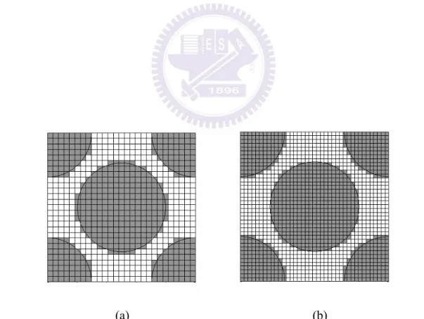
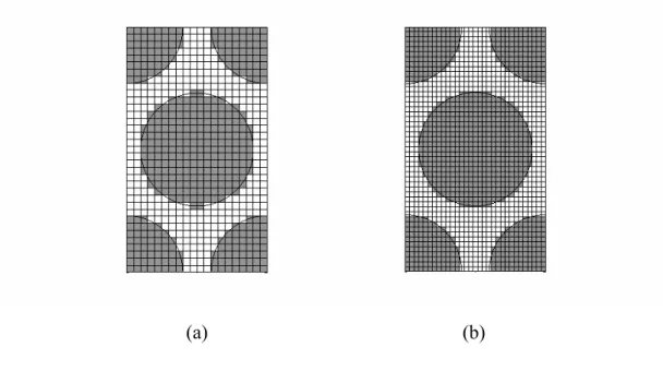
In the GMC analysis, the RVE is divided into the numbers of subcells to represent either fiber or matrix phases. The number of the sub-cells is dependent on the microstructure of the RVE, including fiber geometry and packing arrangement. In general, when a RVE consists of round fibers embedded in matrix, significant amounts of subcells are required in an attempt to precisely simulate the circular geometry of the fiber. However, as more subcells the more computation time is needed. In order to compromise the computation time with the accuracy of the simulation, the converging tests have to be carried out on RVEs with different fiber arrangements arrangement, i.e., square edge, diagonal edge, and hexagonal packing (see Fig. 2.4). Fig. 2.5 demonstrates the RVE with square edge packing, containing 28×28 and 39×39 sub-cells, respectively, where the gray ones denote the fibers, and the white ones are the surrounding matrix. In addition, the RVEs with square

diagonal packing and hexagonal packing were also partitioned into different sub-cells as shown in Figs. 2.6 and 2.7, respectively. Based on the different discretizations of RVEs, the stress and strain curves of the composites with 45° fiber orientation were calculated and the results were then compared in Fig. 2.8. It was shown that for each fiber arrangement, the constitutive curves obtained from the RVEs with coarse sub-cells demonstrate good agreements with those derived from the fine sub-cells. In light of the above verification, it was suggested that the rough partitions of the RVEs have accomplished the converged results and are suitable for characterizing the nonlinear responses of composites with round fibers embedded. The code for calculating the stress and strain curves using the GMC model is attached in Appendix B.

2.4.2 Influence of thermal residual stress on the behaviors of composites

The nonlinear stress strain curves for 15°, 30°, 45°, and 60° fiber composites with different fiber arrays are demonstrated respectively in Figs. 2.9-2.12. For comparison purposes, the composites disregarding the thermal stress effect were also enclosed in the Figures. In the simulations, the temperature change was assumed to be 200 degrees. Results show that the composites with different fiber arrays exhibit different stress and strain curves. Moreover, the square edge packing yields more stiffening behaviors than other fiber packing arrangements. Regarding the thermal stress effect, it is revealed that for the composites with square edge packing, the mechanical behaviors are affected appreciably by the thermal residual stress. Nevertheless, the composites with hexagonal packing and square diagonal packing are relatively less sensitive to the thermal residual stress.

Chapter 3 Comparison of GMC, SCMC and FEM analysis

In Chapter 2 the generalized method cells (GMC) was successful to predict the stress-strain curve on the off-axial loading with three difference fiber arrays. On the other hand, the constitutive relation of fiber composites with different fiber arrays also can be simulated by using the finite element approach such as references [3,4]. From the result of references [3,4], it can observe that when fiber composites apply the off-axial loading the constitutive relation with SEP also exhibit more stiffness then other two fiber arrangements but when fiber composites apply the pure shear loading the constitutive relation with SDP become the most stiffness. In the GMC approach, it can observe the same appearance of constitutive relation when it simulated the off-axial loading but when it apply the pure shear loading the constitutive relation of SEP still the highest stiffness. Because of the GMC exhibits a lack of what is so called “shear-coupling”, which means that the transverse shear stresses on the composites are in general nonzero when the composites are subjected to the transverse tensile loading. This is due to the traction continuity assumption made in the neighboring subcells in the GMC model. Thus, the GMC may product the error result when apply the transverse loading. Hewen et al [15] proposed the strain compatible method of cells (SCMC) model by considering the stress equilibrium in the subcell instead of the continuity constraint in the micromechanical analysis. In this chapter, SCMC model was introduced and the results obtained from the SCMC model were compared with those obtained from GMC and FEM analysis [3].

3.1 Strain compatible method of cells (SCMC)

In the GMC model, the representative volume element (RVE) adopted for the analysis was divided into several subcells. For each subcell, three fundamental assumptions were made, which was described as following

(1) The displacement was continuous between the neighboring subcells in the interface.

(2) The RVE adopted in the analysis must satisfy the periodic boundary condition.

(3) The traction continuity across all cell and subcell interfaces.

It was noted that the first and second assumptions are valid for both GMC and SCMC model. However, the third assumption is modified in the SCMS model by replacing the traction continuity condition with the equilibrium equations such that the stress variation in the adjacent subcell is allowed as well as the transverse stress and shear stress concentration. Through the ingredient constitutive equation, the elasticity equation of equilibrium was expressed in terms of strain components. The equilibrium equations together with the compatibility equations was employed to replace the traction interface continuity given in Eq. (2.1.55) for the derivation of the composite properties.

From the interface displacement continuity condition as derived in the previous chapter, the relation of the local strain and global strain components was written as

η J η A_{G s} = (3.1.1) Where

{

( )11 ( )12 (NN )

}

T s η , η , η η β γ L

= collect the engineering strain rate for

all subcells, and η=

{

η₁₁, η₂₂, η₃₃, 2η₂₃, 2η₁₃, 2η₁₂

}

T represent the overall strain rates of the RVE. In addition, matrices and contain the geometry parameters. Based on the equilibrium condition across the interface of the adjacent subcells, the differential form of the elasticity equilibrium is written as

G

0 x σ x σ 3 13 2 12 ₌ ∂ ∂ + ∂ ∂ (3.1.2) 0 x σ x σ 3 23 2 22 ₌ ∂ ∂ + ∂ ∂ (3.1.3) 0 x σ x σ 3 33 2 32 ₌ ∂ ∂ + ∂ ∂ (3.1.4)

It was note that in the above derivation, the fiber in the unidirectional composites is in the direction and the applied loading is independent of the coordinates. Thus, the derivative of stress components with respective to the direction is equal to zero. With the assistance of the constitutive equation, the equilibrium equation given in Eqs. (3.1.2)-(3.1.4) can be expressed in terms of strain components. In addition, the compatibility conditions originally written as

1 x x₁ 1 x 0 x x η 2 η η η η 3 2 23 2 2 2 33 2 2 3 22 2 = ∂ ∂ ∂ + ∂ ∂ + ∂ ∂ (3.1.5) 0 ) x η x η ( x ₃ 12 2 31 2 = ∂ ∂ + ∂ ∂ − ∂ ∂ (3.1.6) 0 ) x η x η ( x ₂ 31 3 12 3 = ∂ ∂ + ∂ ∂ − ∂ ∂ (3.1.7)

Because all derivatives with respective to are equal to zero, and the strain components was an invariant such that its derivative is zero as well. Integrating Eqs. (3.1.6) and (3.1.7) respectively with and together with the periodic

boundary conditions results in the following relation

1 x 11 η 2 x x₃ 0 x η x η 2 13 3 12 ₌ ∂ ∂ − ∂ ∂ (3.1.8)

and compatibility equation ( Eqs (3.1.5) and (3.1.8) ), all the quantities are assumed to be continuous with the RVE. However, in the SCMC model (GMC model), due to the discrete domain of the RVE, these quantities are not continuous from one subcell to other subcells. Thus, to accomplish the discrete characteristics, the difference equation was replaced using the finite difference approach. For example, regarding to the subcell (1,1) in Fig. 3.1, the equilibrium equation in Eq. (3.1.2) was expressed alternatively as 0 ) l 0.5(l σ σ ) h 0.5(h σ σ 2 1 (1,1) 13 (1,2) 13 2 1 (1,1) 12 (2,1) 12 ₌ + − + + − (3.1.9)

In addition, for the second order partial difference, such as the first two terms shown in Eq. (3.1.5), regarding to the subcell (2,2) in Fig. 3.1 by using central difference approach it was yielded as

) l 0.25(l 0.5l ) l 0.5(l η η ) l 0.5(l η η x η 3 1 2 2 1 (2,1) 22 (2,2) 22 3 2 (2,2) 22 (2,3) 22 2 3 22 2 + + + − − + − ≈ ∂ ∂ (3.1.10)

Furthermore, by using the forward difference and backward difference approach, For example, regarding to the subcell (1,2) in Fig. 3.1, the third term in Eq. (3.1.5) was yielded as ) h )(h l 0.25(l ] η η η [η x x η 2 1 3 2 (1,2) 23 (2,2) 23 (1,3) 23 (2,3) 23 3 2 23 2 + + + − − ≈ ∂ ∂ ∂ (3.1.11)

By means of the finite difference method, the differential forms of the equilibrium and compatibility equations were replaced in the discrete quantities of

each subcell. Based on the periodic boundary condition, there are

independent equations in the equilibrium equations and

independent equations in compatibility conditions. Combination of these equations expressed in term of the local stain components in the subcells leads to

1) N 3(Nβ γ − 1) 1)(N 2(Nβ − γ − 0 η A_{E s} = (3.1.12) where

{

( )11 ( )12 (NN ) T s η , η , η η β γ L

=

}

. As compared to the GMC model, Eq.

(3.1.12) is equivalent to Eq. (2.1.55) which is derived from the interfacial traction continuity condition. In conjunction with displacement continuity condition as given in Eq. (3.1.1), Eq. (3.1.12) becomes

η K~ η A~ _s = (3.1.13) where ; ⎥ ⎦ ⎤ ⎢ ⎣ ⎡ = E G A A A~ _⎥ ⎦ ⎤ ⎢ ⎣ ⎡ = 0 J K~

From now on, the procedure for the derivation of the global constitutive equation of the composites using SCMC is the same as that described in Chapter 2 for the GMC model.

The mechanical properties of the composites were investigated using Finite element approach. The commercial finite element program ANSYS was adopted for the analysis.

3.2.1 Boundary conditions and mesh

In the FEM analysis, the fiber was assumed to be an orthotropic elastic material and the matrix is assuming to be nonlinear material in which the stress and plastic strain curve was determined by a nonlinear function with four coefficients as

) e (1 R ε R k σ p bεp 0 − ∞ − + + = (3.2.1)

where k is the yield stress, and b are parameters which can be determined

properly from the stress and strain curve by following the suggestion provided in the ANSYS manual [14].

0

R R∞

During the FEM analysis, the mechanical behaviors of fiber composite were simulated by considering the representative volume element. The element type was solid-185. In order to characterize the mechanical properties of composites by employing the RVE, the deformation as well as the boundary condition of the RVE needs to be specified properly. In general, the boundary condition was imposed depending on the loading condition and the geometry of the RVE. In this study, we considered the normal stress and the shear stress into the RVE. It is noted that for the applied stresses component , the full model of the RVE need to be accounted for; however, for the other applied stresses, such as , ( ) and ( ), due

to symmetric boundary condition, only a quadrant of the REV was taken into account. In order to describe the appropriate boundary condition according to each loading

23

σ

11

with easy, the coordinate system as well the dimension of the RVE with square edge packing as shown in Fig. 3.2 were utilized hereafter. It should be noted that the following boundary conditions implemented in our simulation were referred to the literature [2, 3].

(1) Stress component with σ₂₃.

Because of non-symmetry stress field, the deformation at ,x ) 2 W , v(x_{1 3} and ) 2 H , x

w(x_{1, 2} was not zero where u, v and w denote the displacement in , and direction, respectively. The associated mesh of RVE for three different fiber arrays were shown in Figs. 3.3-3.5, respectively. Base on the characteristic of periodicity, the boundary condition for this case was given as follows

1 x x₂ 3 x On x₁=0 and x₂=L face ) x , x w(L, ) x , x w(0, ) x , x v(L, ) x , x v(0, constant ) x , x u(L, constant ) x , x u(0, 3 2 3 2 3 2 3 2 3 2 3 2 = = = = (3.2.2) On x₂=0 and x₂=W face ) x , x w(L, ) x , x w(0, ) x W, , v(x ) x ,0, v(x 3 2 3 2 3 1 3 1 = = (3.2.3) On x₃=0 and x₃=H face H) , x , w(x ,0) x , w(x H) , x , v(x ,0) x , v(x 2 1 2 1 2 1 2 1 = = − (3.2.4)

In order to avoid the rigid body motion, the bottom corners was placed on the rollers hence an additional displacement constrain was

0 W,0) , w(x ,0,0) w(x₁ = ₁ = (3.2.5)

(2) Stress component with σ₁₁, σ₂₂(σ₃₃) and σ₁₂(σ₁₃).

Under this stress component field, we only need to analyze quarter of the RVE because of symmetry 0 ) x , 2 W , v(x_{1 3} = ; ) 0 2 H , x w(x_{1, 2} = (3.2.6)

where u, v and w respectively to denote the displacement in , and

direction. Figs. 3.6-3.8 illustrates the finite element mesh of SEP, SDP and HP. Base on the characteristic of periodicity, the boundary condition for this case was given as follows. In the following derivation, the dimension and coordinate system of the simulation box was shown in Fig. 3.9.

On =0 and 1 x x₂ x ₃ 1 x x₁ = face a

(

) (

)

(

) (

)

(

2 3

)

(

2 3

)

3 2 3 2 3 2 3 2 x , x a, w x , x 0, w x , x a, v x , x 0, v constant x , x a, u x , x 0, u = = = − (3.2.7) On x₂=0 and x₂ = face b

(

)

(

)

(

)

(

)

(

a ,b,x

)

w

(

a ,b,x

)

constant w constant x ,0, a w x ,0, a w constant x b, , x v 0 x ,0, x v 3 2 3 1 3 2 3 1 3 1 3 1 = = = = = = (3.2.8)

where a₁ and a₂ indicate any two point with other two identical coordinates. On x₃=0 and x₃ = face c

(

)

(

)

(

) (

)

(

a ,x ,c

) (

v a ,x ,c

)

constant v constant ,0 x , a v ,0 x , a v constant c , x , x w 0 ,0 x , x w 2 2 2 1 2 2 2 1 2 1 2 1 = = = = = = (3.2.9)

In addition, in order to eliminate the rigid body motion, an additional displacement constrain was imposed.

0

u(0,0,0)= (3.2.10)

3.3 Comparison the results of GMC, SCMC and FEM analysis

In GMC, due to the lack of shear-coupling, a direct application of a shear load to a fiber composite will cause the inaccurate result. At this section, the results obtained from GMC, SCMC and FEM will be compared and in order to probe the effect of the shear couple in GMC, the fiber composites subject to the transverse loading . The material properties were given in Table 2.1, where the fiber volume fraction was 60% and those four parameters used in the FEM to simulate the matrix properties were list in Table 3.1. Fig. 3.10 illustrated the matrix stress-strain curves used in the GMC, SCMC and FEM models to ensure that all models have the

22

same matrix properties. Figs. 3.11 shows the stress and strain curves of the fiber composites with three different fiber arrays obtained from GMC and FEM analysis under the transverse loading. It can be seen that there is some discrepancy between these two approaches which could be caused by the shear coupling effect in the GMC analysis. However, the results obtained from the SCMC analysis are in a good agreement with the FEM analysis as illustrated in Figs. 3.12. Based on the above comparison, it seems that the SCMC model can provide more accurate stress and strain curves of the fiber composites under transverse loading.

On the other hand, the significant drawback in the SCMC model is the convergence problem, which was also observed by other researchers [15]. To understand the degree of the convergence in the GMC and SCMC models, we adopted the two meshes, one is coarse and the other is fine, in our simulation for the fiber composites with hexagonal packing under pure shear loading. The results obtained for the GMC and SCMC models are demonstrated in Figs. 3.13-3.14, respectively. Apparently, the GMC model exhibits superior convergence property than the SCMC model. Moreover, in some cases, it is difficult to find the convergence solution in the SCMC analysis. In view of the forgoing, the GMC model still posses its advantage in the convergence issue, although its solution in some cases may not be very accurate. From now on, we will continue to employ the GMC model in the investigation of the mechanical behaviors of the fiber composites, even though some defects exist in the model.

Chapter 4 Effect of fiber array on damping behavior of fiber composites

In this chapter, the GMC model was extended to calculate the fundamental damping properties of fiber composites with different fiber arrays and the damping properties were then implemented as input in the calculation of the modal damping capacity of composite structures with vibrations [13]. The damping behaviors of rod type as well as plate type composites structure constructed based on different fiber arrays will be taken into account in this chapter.

4.1 Damping characterization using GMC

The fundamental damping capacities of fiber composites in material principal directions were calculated by applying a simple loading on the RVE. The RVE used in the previous section was employed to evaluate the stress and strain states of the fiber composites when they were subjected to simple loading. For example, for the calculation of damping properties in longitudinal direction, the unidirectional composites was applied a loading and then through the GMC analysis, the stress states in the fiber and matrix can be evaluated. Based on the energy dissipation concept that the specific damping capacity of material in vibration was defined as the ratio of the dissipated energy and the stored energy for per circle of vibration [11]

U D

ψ= (4.1.1)

the specific damping capacity of the composites can be expressed in terms of damping properties and strain energy of the constituents, i.e. fiber and matrix, as [12]

m f m m f f U U U ψ U ψ ψ + + = (4.1.2)

where ψ_f= specific damping capacity of the fiber ψ_m= specific damping capacity of the matrix U_f= strain energy stored in the fiber

U_m= strain energy stored in the matrix

Thus, the longitudinal damping properties can be calculated from Eq. (4.1.2) directly, once the strain energy as well as the ingredient damping properties was provided. In the fiber composites, the damping behaviors of fiber and matrix were assumed to be isotropic and the corresponding specific damping capacities were listed in Table 4.1. where the data were measured experimentally [17]. As a result, by introducing a simple loading (simple tension, or simple shear) on the RVE, the strain and stress of each subcell was evaluated respectively from Eqs. (2.1.64), (2.1.65) in which

η

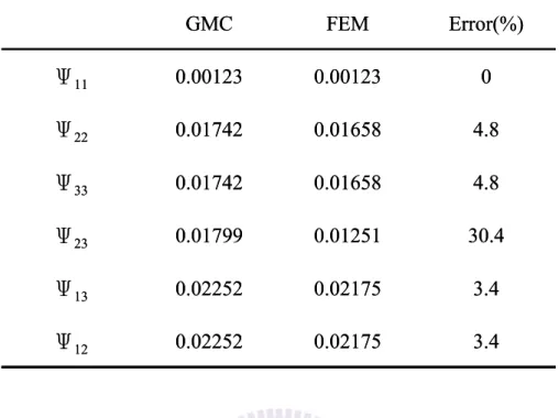
was the overall strain and can be calculated from the constitutive relation of RVE given in Eq. (2.1.67). Moreover, with Eq. (4.1.2), the specific damping capacity of composites in the material directions can be estimated in terms of the damping properties as well as the strain energies of the fiber and matrix phases. Basically the strain energy was computed from the products of the strain and stress states of each subcell associated with either fiber or matrix phases. It is noted that for unidirectional composites, because of the transverse isotropic attribute, only four independent damping properties (ψ₁₁, ψ₂₂, ψ₁₂, ψ₂₃) needs to be calculated.

The damping property of the unidirectional composites with three different fiber arrangements, i.e. square edge packing, square diagonal packing and hexagonal packing, obtained from GMC in conjunction with energy dissipation concept are summarized in Tables 4.2-4.4, respectively. In the calculation, the fiber volume fraction of composites was assumed to be equal to 60%. The damping properties