樹狀物體之分支分析與萃取在文心蘭分級之應用

國

立

交

通

大

學

機械工程研究所

碩士論文

樹狀物體之分支分析與萃取在文心蘭分級之應用

Branch Analysis and Extraction of Tree-Object

on Oncidium Grading

研 究 生： 劉智維

指導教授： 成維華 教授

樹狀物體之分支分析與萃取在文心蘭分級之應用

Branch Analysis and Extraction of Tree-Object

On Oncidium Grading

Submitted to Institute of Mechanical Engineering College of Engineering

National Chiao Tung University in partial Fulfillment of the Requirements

for the Degree of Master

in

Mechanical Engineering November 2005

Hsin-chu, Taiwan, Republic of China

樹狀物體之分支分析與萃取在文心蘭分級之應用

Branch Analysis and Extraction of Tree-Object

On Oncidium Grading

Branch Analysis and Extraction of Tree-Object

On Oncidium Grading

Student：Chih-Wei Liu Advisor：Dr. Wei-Hua Chieng

Institute of Mechanical Engineering National Chiao Tung University

Abstract

Posies are normally presented to consumers in batches. The appearances of these have powerful effect on consumer decision. For this reason, oncidium grading system using pattern recognition is considered. The oncidium shape is segmented from original image. It’s a tree-like image. The “Branch-based region growing” algorithm is applied. It figures out vertices of tree-like image. In this paper, the morphological thinning and branch analysis are presented for solving ambiguous touch and case of crossed branches. After some simplifications and calculation, feature parameters such as length of trunk, length of each branch, count of branch etc. are extracted. Experimental results from artificial and real image are included to demonstrate the validity of the proposed grading methods.

Acknowledgments

I would appreciate my adviser, Professor Wei-Hua Chieng. He guides me to the right way and encourages me to confront my shortcoming in my research during two years. Besides, I am grateful to my seniors in IMLAB specially, one is ABD Chun-Pin Hsu, who teaches me how to analyze a problem, programming skill and point out my mistake for correction.

I thank my family. They support me to finish my study.

Finial, I thank the classmate of our group, Shao-En Sun and Kan-Yoa Chang. They gave me the help for study and advices of research.

CONTENTS 摘 要 ...i Abstract...ii Acknowledgments ...iii CONTENTS ...iv LIST OF FIGURES ...v

LIST OF TABLES ...vi

Chapter 1 Introduction...1

Chapter 2 Oncidium model ...3

2.1 Oncidium grade evaluation...3

2.2 Branch-based region growing...4

2.3 Morphological thinning ...5

Chapter 3 Graph Analysis...9

3.1 Euler’s formula...9

3.2 Graph Search Algorithms ...10

3.3 Graph data structure ... 11

3.4 One dimensional traversal list ...12

3.5 Canonical loop set ...13

Chapter 4 Implement ...14

4.1 Algorithm for region-growing...14

4.2 Path permutation and canonical loop set ...17

4.3 Branch crossing removal ...18

Chapter 5 Experimental results and analysis...20

5.1 Hardware and software...20

5.2 Image acquisition...20

5.3 Preprocess...20

5.4 Image analysis ...21

5.5 Feature extraction and grading ...22

Chapter 6 Conclusion ...24

References ...25

Figures ...27

LIST OF FIGURES

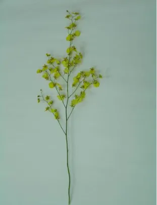
Figure 2.1 Oncidium image...27

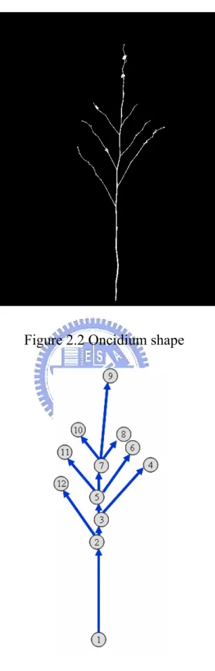
Figure 2.2 Oncidium shape...28

Figure 2.3 Oncidium model...28

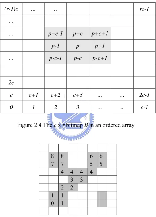
Figure 2.4 The c x r bitmap B in an ordered array ...29

Figure 2.5 Level array data corresponding to a branch based region growing...29

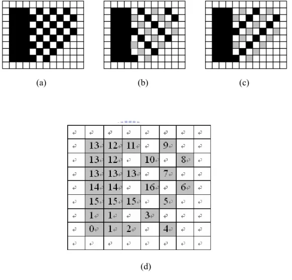
Figure 2.6 Ambiguous branch bifurcation in level array ...30

Figure 2.7 Structuring elements for thinning...31

Figure 2.8 Example of thinning...31

Figure 2.9 Structuring elements for branching detouring...32

Figure 3.1 Example of an undirected graph ...33

Figure 3.2 Complete Depth-first Search (started from π) of an directed graph...33

Figure 3.3 Data structure of a traversal-list ...34

Figure 3.4 Paths of a graph traversal ...34

Figure 3.5 Loop search from a path...35

Figure 3.6 Operation of loops...35

Figure 4.1 Process for Oncidium evaluation ...36

Figure 4.2 Graph of the demo image...37

Figure 4.3 Ambiguous crossed vertices...37

Figure 5.1 Experiment procedure ...38

Figure 5.2 Oncidium simple ...39

Figure 5.3 Gray scale of oncidium image ...40

Figure 5.4 Gray scale of oncidium image ...41

Figure 5.5 Binarization of oncidium ...42

Figure 5.6 Binarization of oncidium ...43

Figure 5.7 (a), (b) Image of merge condition ...44

Figure 5.8 (a), (b) Artificial image ...45

Figure 5.9 (a), (b) Artificial image with crossed vertex ...46

Figure 5.10 (a), (b) Real image of oncidium ...47

LIST OF TABLES

Table 2.1 Oncidium grading ...49

Table 5-1 R, G, B component of oncidium ...50

Table 5-2 Estimation error of figure 5.7 ...51

Table 5-3 Estimation error of figure 5.8 ...51

Table 5-4 Estimation error of figure 5.9 ...52

Table 5-5 Estimation error of figure 5.10 ...52

Chapter 1 Introduction

In recent years, intelligent systems have been employed in applications of automatic grading of gardening products. The advantage of using automatic grading systems instead of manual grading is its ability to be objective and consistent over long period. Grading objects by machine vision is a non-contact and nondestructive method of inspection. The intelligent grading system increases productivity and process efficiency. However, the labor costs by eliminating labor intensive tasks. There are many automatic grading methods have been developed for fruit and vegetables, such as orange, apple, strawberry, tomatoes and cucumbers[12][13][14][15][16][17]. The classifiers of these grading methods included the K-means, fuzzy c-means, K-nearest neighbor, neural network and etc. They separate the fruit and vegetables into several clusters by the features of size, weight, color, shape, length, girth and etc. Shiranita uses a three-layer neural network method to evaluate the distribution of the marbling score of the meat for grading the meat-quality[18]. J. Blasco employs a Bayesian discrimination analysis as the segmentation procedure to separate the target from the background. Thus, quality grading of fruit can be determined by the size and the colorimetric index values of the fruits[19]. The V.Leemans’ method utilized features of apple such as color, shape and texture to evaluate the defective level and grade them[20].

This paper proposed an image analysis approach for estimating length of automatic grading system for oncidium. The appearance of oncidium is very important for consumers. On the other words, the grading system needs to control parameters such as counts of flowers, counts of branches, colors and

etc. In this case, appearance of image is simplified into a direct graph. The approach is using the branch-based method to segment the oncidium’s branch from the background and to search the vertices and arcs of a direct graph [1]. The graphic analysis is also applied to the tree-like branch for the crossed condition. The traversal data are stored in a one dimensional traversal list. Comparing with original data structure of graph, S.Eiho proposes a region-based method for determining the blood vessel segmentation for head MRA image [10]. It’s performed in 3D MRI data. Properly the crossed of branches and the ambiguous touching should be solved. So, the branch analysis and morphological thinning are presented. The morphological thinning is a process of preprocess. It’s produced only for branch-based region growing algorithm. After growing operation, there are many fake arcs and short cuts in the traversal list stored the graph. The traversal list is remodified by merging and permuting process. Experimental results from artificial and real image are included to demonstrate the validity of the proposed grading methods.

Chapter 2 Oncidium model

The oncidium image is shown in Figure 2.1. Its branches are concerned by human. It is a tree-like object made of a main branch, and other sub-branches. It supports that the shape of oncidium after segmenting Figure 2.1 is shown in Figure 2.2. According to the graphic theory, the oncidium shape is expressed into a directed graph with sets of arcs and vertices. The graph is shown in Fig 2-3. There are twelve vertices (v1, v2, v3 …v12) and eleven arcs {(v1, v2), (v2, v3), (v3, v4) … (v2, v12)}. They are registered in traversal list and recognized by computer. According to the traversal list, it is easy to figure out the main branch and sub-branches. For instance, the main branch of Figure 2.3 is {(v1,

v2), (v2, v3), (v3, v5), (v5, v7), (v7, v9)}. The sub-branches are {( v3, v4)}、{( v5,

v6)}、{( v7, v8)}、{( v7, v10)}、{( v5, v11)} and {( v2, v12)}. So the oncidium model is accomplished.

2.1 Oncidium grade evaluation

Oncidium grade evaluation is the finial step of automatic grading system. Every grading system has its inspection rule and classification method according to its features of each product. The features of oncidium are the length of main branch, other branches and a large number of flowers on each branch. The branches are discussed in this paper. The inspection rule shown in Table 2.1 is an example for oncidium grade evaluation. In Table 2.1, the main branch, sub-branch and short branch are defined as follow:

2. Sub-branch: The length of arc is longer than a specific threshold Ls1.

3. Short branch: The length of arc is between threshold Ls1 and Ls2.

Where Ls1 and Ls2 are assigned by grader. An oncidium which main branch

length is measured between 551 and 600 pixels, has four sub-branches and has two short branches is graded to class A. Similarly, oncidium may be graded to class B or C.

2.2 Branch-based region growing

The original image B is an array of pixel values as shown in Figure 2.4. The array represents a two-dimensional image with c width and r height. The first element in that array is the bottom-left element and rest of elements and in stored in raster manner.

The pixel connectivity describes a relation between two or more pixels. For two connected pixel they have to satisfy certain conditions on the pixel brightness and spatial adjacency. To formulate the adjacency criterion for connectivity, the neighborhood functions N4 and N8 may be introduced. The 4-neighbors function N4 returns an ordered list of four elements adjacent to the given element p, i.e.

( ) (

)

4 1, , 1,

N p = p+ p+c p− p c− (2-1)

The 8-neighbors function N8 returns an ordered list of eight neighbor elements around the given element p, i.e.

( ) (

)

8 1, 1, , 1, 1, 1, , 1

N p = p+ p c+ + p c p+ + −c p− p c− − p c p c− − + (2-2)

Those elements are indicated in Figure 2.4.

The branch-based region growing performs the region-growing from one branch to the other. This region growing process starts from the pixel position

labeled with level 0, proceeds to perform the search each pixel position, say p, of all pixel positions labeled with level i, find the foreground pixels in N8(p) and labeled them with level i + 1. In each growing cycle, the connectivity of the region labeled with the same level number is examined against 4-neighbors to find a branch bifurcation. The level indices corresponding to the binary bitmap array is stored in an array denoted by Level. If a growing point reaches a branch bifurcation region, the process continues to grow on only one side of the branches. When the growing point reaches the end of a dangling branch, the growing stops, and then, it starts again from the latest branch bifurcation point. During the growing process, the pixels which are not connected are treated as the branch to be traced later. Figure 2.5 shows an example of the Level array data corresponding to a branch based region growing.

In Fig. 2.5, it is found that, the region growing can only traverse one tree of a possible forest at a time. Thus, after one region growing process, there may be certain regions remained with no level labeled. In such case, multiple region growing processes for the individual trees of a forest are required.

2.3 Morphological thinning

The branch-based region growing suffers the condition of ambiguous touching as shown in Figure 2.6. Figure 2.6(a) shows the original binary image of a plant with sparse branches. When examining Figure 2.6(a), there may be two discrepant interpretations. One interpretation is the plant is pine-tree-like plant with branches pointing to the ground as shown in Figure 2.6(b). The other may be the plant is oak-tree-like plant with branches pointing to the sky as shown in Figure 2.6(c). Such confusion will also induce problems of the branch bifurcation during the process of region-growing. In Figure 2.6(c), the level

labeling are confusing for intuitively distinguish the branches. The problem occurs at the low resolution for some thin branches. These thin branches causing confusion may be removed by the following thinning operations.

Thinning is a morphological operation that is used to remove selected foreground pixels from binary images. The thinning operation is related to the hit-and-miss transform. The behavior of the thinning operation is determined by a structuring element. The binary structuring elements used for thinning are of the extended type described under the hit-and-miss transform. Note that the structuring element must always have a one or a blank at its origin if it is to have any effect. The thinning of an image B by a structuring element J is:

( , ) ( , )

thin B J = −B hit−and−miss B J (2-3)

where the subtraction is a logical subtraction defined by ~

B Y− = ∩B Y (2-4)

The thinning operation is calculated by translating the origin of the structuring element to each possible pixel position in the image, and at each such position comparing it with the underlying image pixels. If the foreground and background pixels in the structuring element exactly match foreground and background pixels in the image, then the image pixel underneath the origin of the structuring element is set to background (zero). Otherwise it is left unchanged. In fact, the operator is normally applied repeatedly until it causes no further changes to the image, i.e. convergence. In this paper, the physical dimensions of the oncidium as stated in Chapter 2 are important parameters for evaluating the grade of the oncidium. The thinning structuring element introduced in this paper is only for removing the ambiguous touching of

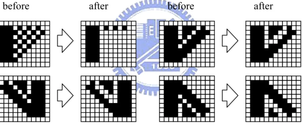
branches that cause the confusion on level labeling, which should not account for producing the skeleton of the oncidium. The structuring elements may be schematically shown in Figure 2.7. The origin of the structuring element of Figure 2.7(a) is at the bottom-left corner and that of Figure 2.7(b) is at the bottom-right corner. The examples of thinning are shown in Figure 2.8. It is observed from Figure 2.8 that the result of the thinning operation is symmetrical in horizontal direction but not in the vertical direction. The thinning operation can separate the ambiguous touching of the branches; however, the unwanted forest is also produced. These unconnected regions due to the weak connectivity of the branches may be ignored after the first branch-based region growing process starting from the root of the tree.

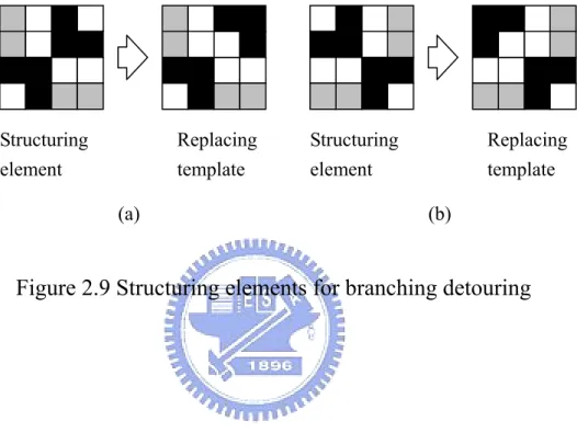
The intuitive question is arisen that should the operator be applied until the convergence. If the pixel position, say p, is set to background (zero) due to a hit of Figure 2.7(a), then it may potentially result the 8-connected image centered at p form a hit due to structuring element as shown in Figure 2.7(b). In such case, the repeated application of the thinning operator may gradually destroy the connectivity of the branches. To avoid this effect of backward propagation, the branch detouring operation, as shown in Figure 2.9, shall be performed before the aforementioned thinning operation.

The branch detouring operation is calculated by translating the origin of the structuring element to each possible pixel position in the image, and at each such position comparing it with the underlying image pixels. If the foreground and background pixels in the structuring element exactly match foreground and background pixels in the image, then the image pixels underneath the origin of the structuring element are set to the replacing

template. The branch detouring operation has prevented the occurrence of the back propagation of thinning operation. Thus the convergence at single thinning operation can be achieved.

Chapter 3 Graph Analysis

The branch relation of a plant under a 2-D image projection may be represented by the graph. A graph is a mathematical abstraction that is useful for solving many kinds of problems. Fundamentally, a graph, as shown in Figure 3.1, consists of a set of vertices, and a set of edges, where an edge is something that connects two vertices in the graph. More precisely, a graph is a pair (V, E), where V is a finite set and E is a binary relation on V. V is called a vertex set whose elements are called vertices. E is a collection of edges, where an edge is a pair (v1, v2) with both v1, v2 in V. In a directed graph, edges are

ordered pairs, connecting a source vertex to a sink vertex. In an undirected graph edges are unorderly pairs and connect the two vertices in both directions, hence in an undirected graph (v1, v2) and (v2, v1) are two ways of writing the

same edge.

3.1 Euler’s formula

In graph theory, a planar graph is a graph that can be embedded in the plane so that no edges intersect. Euler's formula states that if a finite connected planar graph is drawn in the plane without any edge intersections, and v is the number of vertices, e is the number of edges and f is the number of cycle, then

2

f + = +v e (3-1)

Euler's formula can be proven as follows: if the graph isn't a tree, then remove an edge which completes a cycle. This lowers both e and f by one, leaving v −

e + f constant. Repeat until you arrive at a tree; trees have f = 1 and

1

In a finite connected simple planar graph, any cycle is bounded by at least three edges and every edge touches at most two cycles; using Euler's formula, one can then show that these graphs are sparse in the sense that e ≤ 3v - 6 if v ≥ 3. A vertex has degree n if there are n edges connecting that vertex to other vertices. The vertex with degree is 1 called the dangling vertex.

The graph in Fig. 3.1 employs six vertices and nine edges, i.e. v = 6 and e = 9. From the Euler’s formula, it is obtained that f = e − v + 2 = 5, which is identical to the number of faces shown in Fig. 3.1. The degree of vertices a, y,

is 4. The degree of vertex b is 3. The

　 degree of vertex x is 2. The degree of vertex z is 1 hence it is a dangling vertex.

3.2 Graph Search Algorithms

Tree edges are edges in the search tree (or forest) constructed implicitly or explicitly by running a graph search algorithm over a graph. An edge (v1, v2)

is a tree edge if v2 was first discovered while exploring edge (v1, v2). Back

edges connect vertices to their ancestors in a search tree. So for edge (v1, v2)

the vertex v2 must be the ancestor of vertex v1. Self loops are considered to be

back edges. Forward edges are non-tree edges (v1, v2) that connect a vertex v1

to a descendant v2 in a search tree. Cross edges are edges that do not fall into

the above three categories.

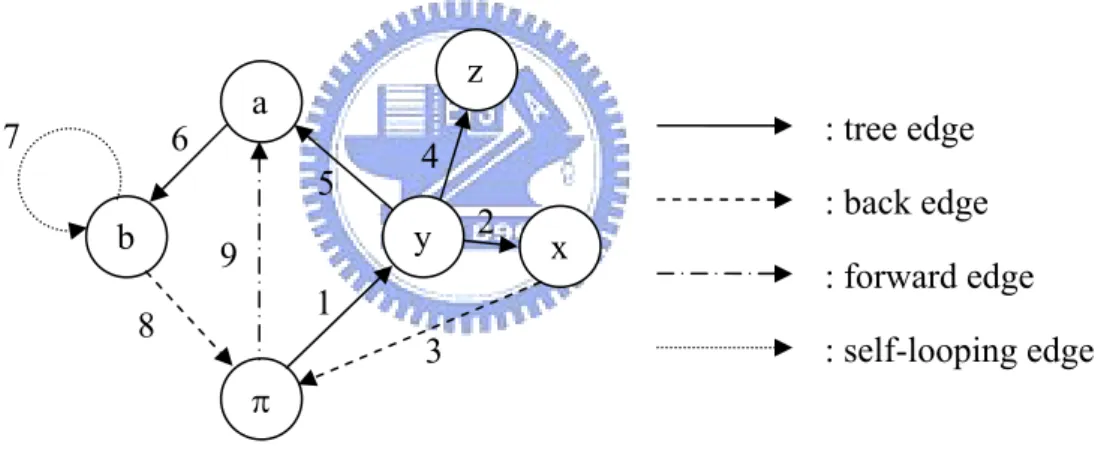
The conventional depth-first search (DFS) visits only all the vertices in a graph and ignores the edges. Thus, no re-visit of any vertex is necessary. In our application, it needs to visit all edges of the graph since each edge represents a branch of the oncidium. We then modify the depth-first search into a complete depth-first search (CDFS) which visits all the edges and vertices in a graph. By choosing which edge to explore next, this algorithm always chooses to go

deeper into the graph. That is, it will pick the next unvisited edge until reaching a vertex that has only a single edge. The algorithm will then backtrack to the previous vertex and continue along any as yet unexplored edges from that vertex. After CDFS has visited all the reachable edges and vertices from a particular source vertex, it chooses one of the remaining undiscovered edges and continues the search. This process creates a set of depth-first trees which together form the depth-first forest. A depth-first search categorizes the edges in the graph into three categories: tree-edges, back-edges, self-looping, and forward edges. Fig. 3.2 depicts the depth first search of the graph in Fig. 3.1. The edges in Figure 3.2 are ordered by discover time.

3.3 Graph data structure

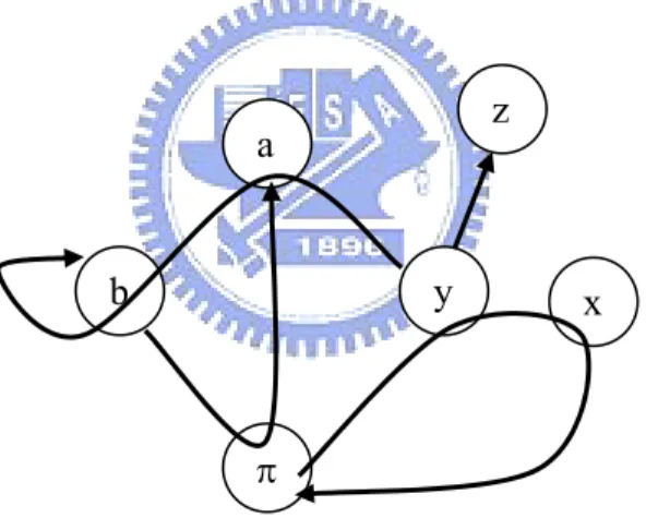
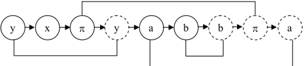
The primary property of a graph to consider when deciding which data structure to use is sparsity, the number of edges relative to the number of vertices in the graph. A graph where e is close to v2 is a dense graph. A traversal-list representation of a graph stores the edge sequence of traversal of that graph based on CDFS. If we use an open-parenthesis when a vertex is traversed and a close-parenthesis when a vertex is finished, then the result is a properly nested set of parenthesis. The traversal-list started from of the 　 CDFS graph in Fig. 3.2 may be represented as

( ( ( ) ( ) ( ( ( ) ( ( ))))))

T = π y x π z a b b π a (3-3)

The traversal-list is a list of lists. Each open-parenthesis of the traversal-list corresponds to the head of an individual directed edge. Each closed-parenthesis of the traversal-list corresponds to the tail of an individual directed edge. The data structure of the above traversal-list is shown in Fig. 3.3;

there are totally nine pointers of list, each of them corresponds to an open parenthesis and nine pointers of cons, each of them corresponds to a closed-parenthesis, required to store the CDFS graph. The traversal-list needs a memory to store 2e pointers and e + 1 vertex data.

3.4 One dimensional traversal list

The traversal-list may be may be stored in an array, called the one dimensional traversal list, by replacing the closed-parenthesis into a partition symbol, for instance “。”, and eliminating all open-parenthesis as follows.

( )

T = π y x π D y z Dy a b b D b π aD D D D D D (3-4)

In the above expression, the closed parenthesis at the end positions of the list can be ignored. Thus, it is convenient to write

( )

T = π y x π D y z Dy a b b D b π a

a

(3-5) The traversal-array expression corresponds to the paths of the graph traversal

is shown in Fig. 3.4.

By ignoring the discover time of each path, the paths in the one dimensional traversal list may be commutated to represent exactly the same graph as follows. For example, we relocate the path (y z) to the end of the traversal list

( )

T = π y x πDy a b b D bπ (3-6)

The paths may also be permutated so that one of the paths covers more vertices. For example,

( )

T = y x π D π y a b b D b π a D y z (3-7)

( )

T = y x π D π y a b b D b π a D y z

( )y x π y a b b π a y z

= D (3-8)

3.5 Canonical loop set

According to the traversal list, it is easy to verify that the degree of vertices a, y, π is 4 for each of them has 4 edges connecting that vertex to other vertices. The degree of vertex b is 3. The degree of degree of vertex x is 2. Vertex z is a dangling vertex. The dangling vertex is the oncidium image corresponds to the end point of the dangling branch. A face forms a loop in the graph except for the outer face. The number of loops l is equal to the number of faces f minus 1. The traversal list is useful in the task of loop-search. By comparing the proceeding vertex to the previous vertices in the traversal list, individual loops are identified as depicted in Fig. 3.5. There are four loops identified from Fig. 3.5 which complies with the relation that l = f – 1 = 5 – 1 = 4. The four loops are ( )y x π y , ( )π y a bπ , ( )b b , and ( )a π b a . By adding

or subtracting the loops, we are able to reduce the length of the subject loop. For example, ( )π y a b π + ( )a π b a = ( )π y a b π , the operation is shown

schematically in Figure 3.6. The canonical loop set is derived from performing continuously the reduction of loop length until none of the loop can have further reduction.

Chapter 4 Implement

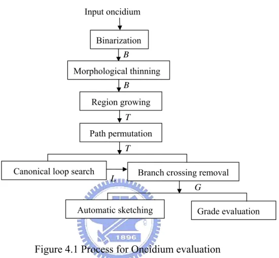
The algorithm for the oncidium grade evaluation is composed of steps as follows.

1) perform the image binarization to obtain array B,

2) perform the morphological thinning to the image array B,

3) perform the branch-based region growing to obtain traversal-list T, 4) perform the path permutation to find the maximum length of paths A, 5) perform the canonical loop search to obtain L,

6) perform the branch crossing removal to obtain G, and

7) sketch the skeleton oncidium and perform the grade evaluation. The flow control of the algorithm is shown in Fig. 4.1.

4.1 Algorithm for region-growing

The region growing given in this paper is according to the branch-based region growing. The algorithm is provided with the global memory of a traversal list T and BUFFER and SEARCH lists. All of the lists are set to empty in the beginning. The array Level storing the level labeling data array is also declared as a global memory. T will be stored with the level number, i.e. the vertex number is the level number, of the graph representing the oncidium tree. The function CheckLoop searches for the loop found in the graph search. For example, if Level(p) = π is input to the function CheckLoop when

( )

The pseudo-code implementation of the function CheckLoop is given as follows.

CheckLoop( p)

¾ Input: p is a pixel position if (Level(p) is in the T list) { 1

Declare an integer r and set r to be the value of the tail vertex of T list 2

if (r≠ Level(p)) then put Level(p) on the tail of T list }

3

Corresponding to the branch-based region growing algorithm stated in chapter 2.2, in every growing cycle the connectivity of the region labeled with the same level number is examined against 4-neighbors to find a branch bifurcation. The function LevelGrow takes two pixel positions, for instance p and p1, and compares their 4-neighbors conditions as well as the level number to determined where they are in the same level and 4-neighors related. The

BUFFER list stores all pixel positions in the current level of search. The empty BUFFER indicates a new level of search is started. Since the 8-neighbors

function N8 will yield an ordered list with proper adjacency, the condition of the same level and 4-neighors related may be performed by the intersection of N4(p) and the BUFFER list. The pseudo-code implementation of the function

LevelGrow is given as follows.

LevelGrow(p1,cycle)

¾ Input: p and p1 are pixel positions ¾ Output: TRUE or FALSE

if BUFFER list is empty .or. 1

p is in the intersection list of N4 (p1) and BUFFER list { 2

3 Set Level(p1) to be Cycle

4 Put p1 on BUFFER list

return TRUE } 5

else return FALSE 6

The SEARCH list is set to empty in the beginning. SEARCH list is used to store the temporary vertex information of region growing. This region growing process starts from the pixel position labeled with level 0, proceeds to perform the search each pixel position, say p, of all pixel positions labeled with level i, find the foreground pixels in N8(p) and labeled them with level i + 1. The function RegionGrow is used for growing the regions in the sense of the complete depth-first search (CDFS). In case that the connectivity doesn’t hold for certain level of growing, the branch bifurcation is found in that level. When the growing point reaches the end of a dangling branch, the growing stops, and then, it starts again from the latest branch bifurcation point. The

BUFFER_LIST will be added to the search list whenever a level growing is

completed. The region growing stops whenever the SEARCH_LIST is empty. The pseudo-code implementation of the function RegionGrow is given as follows.

RegionGrow (p)

¾ Input: p is the starting pixel position

Set all elements in Level to be -1 except for Level(p) to be 0 1

Set SEARCH list empty and put p on the SEARCH list 2

3 Set T list empty and put Level(p) on the T list

4 Set Cycle to be 1

while the SEARCH list is not empty { 5

6 Declare Boolean BRANCH_BIFURCATION and LEVEL_COMPLETED 7 Set BRANCH_BIFURCATION and LEVEL_COMPLETED to be FALSE

Get the head vertex off SEARCH list and call it p 8

9 Remove the head vertex of SEARCH list for p1 in N8(p) { // 8-connected neighborhood 10

if (B(p1)≠0) then CheckLoop(Level; p1) 11

if (LevelGrow(Level; p; p1) ≠ TRUE && Level(p) == -1) { 12

13 Set BRANCH_BIFURCATION to be TRUE 14 Put p1 on the head of the SEARCH list

15 Put Level(p) on the tail of the T list

16 Break the loop}} if not BRANCH_BIFURCATION { 17

18 Declare q and set q to be the value of the head vertex of SEARCH list if Level(p) != Level(q) Set LEVEL_COMPLETED to be TRUE } 19

else if the SEARCH list is empty Set LEVEL_COMPLETED to be TRUE 20

if (BRANCH_BIFURCATION or LEVEL_COMPLETED) { 21

Merge BUFFER list to the head of SEARCH list 22

23 Set BUFFER list empty 24 Set Cycle to be (Cycle + 1)}}

An example of region growing is shown in Fig. 4.2.

4.2 Path permutation and canonical loop set

The one dimensional traversal list obtained from the function

RegionGrow is that

(0 5 912 9151619 16 23 16 26 28 29 33 29 36 29 5 26)

Since neither level number 15 nor 16 is an end point of the dangling branch, the level number 15 and 16 can be merged together. Following the similar line reasoning, the level number 28 and 29 can be merged together. The traversal list is simplified into

(0 5 912 91619 16 23 16 26 29 33 29 36 29 5 26)

T = D D D D D (4-2)

The paths in the traversal list may be permutated to increase length of the path with the starting level 0, for instance

(0 5 91619 912 16 23 16 26 29 33 29 36 29 5 26)

T = D D D D D (4-3)

The path permutation may go further to find

(0 5 9 16 26 29 5 26 9 12 16 23 16 19 29 36 29 33)

T = D D D D D (4-4)

The canonical loop set may be verified that

4.3 Branch crossing removal

The canonical loop set is described above in chapter 3.5. In each canonical loop set, there is a crossed vertex in it. The crossed vertex has two features. Its degree is bigger than 4 and even. Thus, the degrees of crossed vertex should be four, six, eight or more. The vertices on canonical loop set satisfied those conditions are few. The crossed vertex can be figured out generally. It is a mistake that oncidium graph exists the crossed vertex. It is replaced with two crossed arcs. By comparing the slope of arcs connecting with crossed vertex, the couple of arcs with similar slope are combined. The traversal list is permuted for satisfying the Euler formula. Sometimes, it is not only one vertex satisfying all properties shown in Figure 4.3. The vertex 5 and vertex 29 are both in the canonical loop set (5 26 29). Their degrees are four. They are ambiguouscrossed vertices. Which one should be removed depends on

comparing the slope of them. Then, choose the better one. For Figure 4.3 canonical loop set (5 26 29), comparing the result of vertices 5 and 29, the similarity of slopes of connecting arcs {(5 29), (29 33)} and {(26 29), (29 36} of vertex 29 is better than connected arcs {(0 5), (5 26)} and {(5 9), (5 29)} of vertex 5. Thus, the vertex 29 is removed. Canonical loop set (5, 26, 29) is destructive. It’s replaced with arcs (5, 33) and (26, 36). The traversal list is permuted. The canonical loop set (5, 9, 16, 26) is either. The branch crossed removal finished.

Chapter 5 Experimental results and analysis

5.1 Hardware and software

The environment of hardware is a personal computer (PC) of AMD Athlon(tm) XP 1.81GHz with 256MB RAM. The entire algorithm for automatic inspection system of oncidium has been implemented in C++ language to run in the Visual C++ 6.0 environment. The sample image is a 640(h)×480(v) pixels, 24 bit color image. The finial result is presented of five stages shown in Figure 5.1 and is descript as follow.

5.2 Image acquisition

The image is acquired by a CCD camera. The diaphragm and shutter of CCD camera is set to F3.2 and 1/20 second. There are some sample images shown in Figure 5.2.

5.3 Preprocess

The shape of oncidium branches is segmented by gray scale and binarization. The gray scale is processed by the image process software. The image is separated into the independent R, G and B components. The gray scale image is given by

W = × + × + ×α R β G γ B (5-1)

By analyzing original image, the R, G, B components of flowers, branches and background are extracted shown in Table 5-1. The blue components of flower and background are close. The easiest gray scale is set

(

)

(

)

The result image of gray scale image is shown in Figure 5.3 and Figure 5.4. There are two real images. The binarization technique is used to isolate objects of interest having values different from the background. Each pixel is classified as either belonging to an object of interest or to background. This is accomplished by assigning to a pixel the value 1 if the source image value is within a given threshold range and 0 otherwise. The binarization procedure is immediate. Let x be the source image and

R

a∈

[ ]

range. The binarization image

{ }

b∈ 0,1 is given by 1 if h a(x) k ( ) 0 otherwise b x = ⎨⎧ ≤ ≤ ⎩ (5-2)

The parameters

[ ]

[

]

shown in Figure 5.5 and Figure 5.6.

5.4 Image analysis

The image analysis can be divided into three procedures: 1) we carried out 8-connected branch-based region growing for binarization image and the traversal list is generated. 2) The traversal list merged and permuted. The merge procedure needs to set a threshold. It’s called d set to be 20, here. It solves the problems of deckle edge and fake arcs shown in Figure 5.7(a), (b). If the d set too small, the algorithm determines overmuch short branches. If the d is too big, arcs which length small than d are ignored. But the more accurate coordinates of vertices always brings smaller error. 3) The traversal list is examined by Euler formula. 4) if Euler formula showed there are loops in graph, the crossed vertex must be removed by permuting the traversal list. The some results are shown in Figure 5.8, Figure 5.9, Figure 5.10 and Figure 5.11. There are two artificial

images and two real images. The searching vertices are marked by circle with purple color and given an index for travel order. There is canonical loop set in Figure 5.9 and Figure 5.11. All crossed vertices are removed as figure. In figure 5.11, the traversal list is {0 209 252 348 394。348 470。348 590 639 659 706。 659 893。639 1126。590 1188 252。1188 1359。209 1505} before the crossed vertex is removed. There is a feedback arc (1188 252) and canonical loop set (252 348 590 1188). The vertex 348 is crossed vertex. After crossed vertex removing, the traversal list is {0 209 252 1188 590 639 659 706。659 893。639 1126。590 394。1188 1359。252 470。209 1505}. The main branch list is (0 209 252 1188 590 639 659 706). Other branches are (659 893), (639 1126), (590 394), (1188 1359), (252 470) and (209 1505). The vertex 348 is removed. There is no canonical loop set in it. The traversal list is remodified.

5.5 Feature extraction and grading

The length of main branch and other branches are extracted. The estimation error is given by

100%measurement estimation branch error measurement − ⎛ = ⎜_{⎝ ⎠}⎞×⎟ (5-3)

(

)

average error=average branch error (5-4)

The errors of main branch and sub-branch of Figure 5.8, Figure 5.9, Figure 5.10 and Figure 5.11 is shown in Table 5-2, Table 5-3, Table 5-4 and Table 5-5. The average error of total experiments is shown in Table 5-6. The sub-branch estimation errors of artificial image are about 10% to 15% but main branch estimation error is very low. It seems bad for artificial images. For pixel error

point of view, main branch and sub-branches are approximate. Where the pixel error means . The same pixel errors are divided by different measurement values. When measurement value is as large as main branch, the estimation error is smaller. The estimation error of a main branch is the smallest for each oncidium therefore. It is opposition to sub-branch error. The denominators of sub-branch error are smaller, so the bigger errors are obtained. The pixel error is generated by the averaged value of vertex center and merge operator.

Chapter 6 Conclusion

The paper proposed an efficient image analysis method of tree-object image and oncidium image by graphic analysis. The approach essentially based on digital image process combining graphic analysis theory. The graphic analysis providing a solution for crossed branches of 2-D projection image. It solves the endless problem of 2-D projection image. It improves the visual ability of computer for recognition oncidium. The morphological thinning efficiently solved the ambiguous touch for branch-based region growing algorithm. But in reduction image, it may cause branch cutoff. This proposed method is applied in oncidium inspection. The main branch error is 3.59%, and the sub-branch error is 10.2% shown in Table 5-6. A good grading system isn’t inspection of products for only one parameter. In this paper, the accuracy is ignored. Because the only parameter of length is discussed, but there are more parameters such as the number of flowers and flowers color need to be added in the grading system. Further, the trend of branches can be controlled. Besides, the segmentation result influences the error of experiment. If the image segmentation result is more correct, the smaller merged threshold could be set. And the result of error would be reduced. Such as Figure 5.10(a) and Figure 5.11(a), they are acquisited by one oncidium. There is a canonicall loop in Figure 5.11 but Figure 5.10 isn’t. After branch analysis, the traversal lists of them are different, but the same counts of sub-branches and the close estimation length of branches are obtained.

References

[1] John M. Boyer and Wendy J. Myrvold (2005). On the cutting edge: Simplified O(n) planarity by edge addtion. Journal of Graph Algorithms and Applications, vol. 8 no. 3, pp. 241-273.

[2] Colbourn, C. J. and Dinitz, J. H. (1996). CRC Handbook of Combinatorial Design. Boca Raton, FL: CRC Press.

[3] R. Gonzalez and R. Woods Digital Image Processing, Addison-Wesley Publishing Company, 1992, pp 518 - 548.

[4] E. Davies Machine Vision: Theory, Algorithms and Practicalities, Academic Press, 1990, pp 149 - 161.

[5]R. Haralick and L. Shapiro Computer and Robot Vision, Vol 1, Addison-Wesley Publishing Company, 1992, Chap. 5, pp 168 - 173.

[6] Scott E Umbaugh, “Computer Vision Image Processing”, Prentice Hall, International Editions, 1998.

[7] Robert M. Haralick, “Computer and Robot Vision Volume 1”, Addison-Wesley Publishing, 1992.

[8] Gerhard X. Ritter, Joseph N. Wilson, “Computer Vision Algorithms in Image Algebra”, CRC Press, 1996.

[9] Rafael C. Gonzalez, Richard E. Woods, “Digital Image Processing” Prentice Hall, Pearson International Edition, 2002.

[10] S.Eiho, H.Sekiguchi, N.Sugimoto, “Branch-based Region Growing Method for Blood Vessel Segmentation”, Graduate School of Informatics,

Kyoto University, Gokasho, Systems and Computers in Japan, Volume 36, Issue 5, pp 80-88.

[11] 廖紹綱, “數位影像處理”, 全華科技圖書, 1996.

[12] U. Ben-Hanan, K. Peleg, and P. Gutman, “Classification of fruits by a Boltzmann perceptron neural network,” Automatica, vol. 28, pp. 961–968, 1992. [13] B. K. Miller and M. J. Delwiche, “Peach defect detection with machine vision,” Trans. Amer. Soc. Agricultural Eng., vol. 34, pp. 2588–2597, 1991. [14] N. J. C. Strachan, “Length measurement of fish by computer vision,” Comput. Electron. Agriculture, vol. 3, pp. 93–104, 1993.

[15] M. S. Howarth, J. R. Brandon, S. W. Searcy, and N. Kehtarnavaz, “Estimation of tip shape for carrot classification by machine vision,” J. Agriculture Eng. Res., vol. 53, pp. 123–139, 1992.

[16] N. Sarkar and R. R. Wolfe, “Computer vision based system for quality separation of fresh market tomatoes,” Trans. Amer. Soc. Agricultural Eng., vol. 28, pp. 1714–1718, 1985.

[17] W. M. Miller, “Classification analysis of Florida grapefruit based on shape parameters,” in Proc. Amer. Soc. Agricultural Eng. Food Processing Automat., Lexington, KY, May 1992, pp. 339–347.

[18] K. Shiranita, K. Hayashi, A. Otsubo, T. Miyajima, R. Takiyama, Meat quality evaluation method by image analysis and its applications, Pattern Recognition 33 (2000) 97-104.

[19] J. Blasco, N. Aleixos, E. Molt, Machine Vision System for Automatic Quality Grading of Fruit, Biosystems Engineering 85(4) (2003) 415-423.

[20] V. Leemans, M.-F. Destain, A real-time grading method of apples based on features extracted from defects, Journal of Food Engineering, 61 (2004) 83-89

Figures

Figure 2.2 Oncidium shape

(r-1)c … .. rc-1 … … p+c-1 p+c p+c+1 p-1 p p+1 … p-c-1 p-c p-c+1 2c c c+1 c+2 c+3 … … 2c-1 0 1 2 3 … .. c-1

Figure 2.4 The c x r bitmap B in an ordered array

8 8 6 6 7 7 5 5 4 4 4 4 3 3 2 2 1 1 0 1

(b)

Figure 2.6 Ambiguous branch bifurcation in level array

(a) (c)

Figure 2.7 Structuring elements for thinning

before after before after (b)

(a)

Replacing template Replacing template Structuring element Structuring element (a) (b)

Figure 3.1 Example of an undirected graph

Figure 3.2 Complete Depth-first Search (started fromπ) of an directed graph

a b y π x z 1 2 3 4 5 6 7 8 9 : tree edge : back edge : forward edge : self-looping edge a b y π x z

Figure 3.3 Data structure of a traversal-list

Figure 3.4 Paths of a graph traversal

a b y π x z a b y π x z π b π a : pointer of a list : pointer of a cons

Figure 3.5 Loop search from a path

a

Figure 3.6 Operation of loops

b y

π

a b

Binarization

Region growing

Figure 4.1 Process for Oncidium evaluation

Path permutation

Canonical loop search Branch crossing removal

Automatic sketching _{Grade evaluation} Input oncidium B T T L G Morphological thinning B

Figure 4.2 Graph of the demo image

Figure 4.3 Ambiguous crossed vertices

0 5 9 12 19 16 23 33 36 29 26 0 5 9 12 19 15, 16 23 33 36 28, 29 26

Image acquisition

Image analysis Preprocessing

Feature extraction

Register and grading

(a) (b) (c)

(d) (e) (f) Figure 5.2 Oncidium sim le p

(a)

e condition (a) Fake arc

(b)

Figure 5.7 (a), (b) Image of merg

(a)

(b)

Figure 5.8 (a), (b) Artificial image (a) Original image

(a)

(b)

Figure 5.9 (a), (b) Artificial image with crossed vertex (a) Original image

(a)

(b)

Figure 5.10 (a), (b) Real image of oncidium (a) Original image

(a)

(b)

Figure 5.11 (a), (b) Real image with crossed vertex of oncidium (a) Original image

Tables

Level Length of primary branch Amount of sub-branch Amount of short branch Case A 551~600Pixel 4 2 Case B 501~550Pixel 3 3 Case C 451~500Pixel 2 4

Flowers branches background Red 120-150 20-50 130-160 Blue 140-160 50-70 160-180 Green 0-30 10-50 145-165

Estimation length (mm) Measure length (mm) Error of each branch (%) Average error (%) Main branch 215.23 217 0.81 78.93 (4-14) 68 16.07 58.64 (7-13) 51 14.99 28.48 (10-12) 25 13.95 50.35 (8-9) 44 14.44 85.47 (5-6) 77 11.00 Sub-branch 93.78 (2-3) 11.84 84 11.64 T ation r of figure 5.7 Estimation (mm) Measurement (mm) Error of each branch (%) Average error (%) able 5-2 Estim erro

Main branch 206.32 208 0.80 91.40 (3-5) 84 8.81 Sub-branch

69.55 (3-4) 67 3.81

4.47

Estimation length (mm) Measure length (mm) Error of each branch (%) Average error (%) Main branch 206.44 208 0.74 59.25(3-4) 51 -16.19 32.74(6-7) 33 0.77 28.46(8-9) 22 -29.37 25.75(8-11) 30 14.16 47.84(5-12) 45 -6.32 Sub-branch 52.28(2-13) 10.61 49 -6.70 Table 5-4 Estimat rror of fi .9

Estimation Measure Error of each Average error (%) ion e gure 5

length (mm) length (mm) branch (%) Main branch 196.07 208 5.73 60.81(3-13) 53 -14.75 36.8(5-11) 33 -11.51 21.27(7-8) 24 11.37 26.89(6-10) 30 10.34 47.70(4-12) 45 -6.01 Sub-branch 45.43(2-14) 1 10.09 51 0.91 Table 5-5 Estimation error of figure 5.10

Type Error Main branch 3.59%

Sub-branch 10.2% Table 5-6 Average error of oncidium