行政院國家科學委員會專題研究計畫 期末報告
最適政府支出融通政策:銀行與股市金融體系之比較
計 畫 類 別 : 個別型 計 畫 編 號 : NSC 101-2410-H-004-012- 執 行 期 間 : 101 年 08 月 01 日至 102 年 10 月 31 日 執 行 單 位 : 國立政治大學經濟學系 計 畫 主 持 人 : 洪福聲 共 同 主 持 人 : 蔣世中 計畫參與人員: 碩士級-專任助理人員:陳建印 博士班研究生-兼任助理人員:陳冠彰 博士班研究生-兼任助理人員:林朕陞 公 開 資 訊 : 本計畫涉及專利或其他智慧財產權,2 年後可公開查詢中 華 民 國 102 年 11 月 26 日
中 文 摘 要 : 本計畫原先希望比較政府支出融通在銀行體系與股票市場體 系的差異。然而,結果的差異不大。我們因此將研究重心轉 向,探討當金融市場存在訊息不對稱時,比較政府貨幣融通 與課稅融通的相對好處。結果發現,訊息不對稱對於政府支 出融通政策效果扮演一個很重要的角色。我們首先建立,政 府支出比例大小對於資本投資是否受到限制,扮演重要角 色。當政府支出比例較大時,資本投資受到限制,此時,課 稅融通比貨幣融通要佳。反之,貨幣融資較佳。本研究除了 對政府融通政策效果有清楚的分析外,模型結果也與一些實 證研究相符。 中文關鍵詞: 訊息不對稱、信用限額、政府支出融通、內生成長
英 文 摘 要 : Originally, we intend to compare the relative merits of government expenditure financing under financial markets with banking and stocking systems,
respectively. Nonetheless, it turns out that results are not so interesting, compared with recent
empirical studies. We then turn our attention to compare relative merits of financing with the presence of asymmetric information. We first
establish that the share of government expenditure determines whether or not credit is rationing, which in turn plays an important role in determining the relative merits of money and income-tax financing. It is found that money financing leads to both higher inflation and economic growth than income-tax financing if credit is non-rationing. If credit is rationing, however, money financing leads to a higher inflation rate but a lower growth rate than tax
financing. In comparing social welfare, we find that money (tax) financing is better than income-tax (money) if credit is non-rationing (rationing). Our results reconcile the pre-existing literature and are consistent with some empirical evidence.
英文關鍵詞: Asymmetric Information, Credit Rationing, Money and Income-tax Financing, Endogenous Growth
1
行政院國家科學委員會補助專題研究計畫
期末報告
最適政府支出融通政策:銀行與股市金融體系之比較
計畫類別:個別型計畫
計畫編號:NSC101-2410-H-004-012
執行期間: 2012 年 08 月 01 日至 2013 年 10 月 31 日
執行機構及系所:
政治大學經濟系
計畫主持人:洪福聲
共同主持人:蔣世中
計畫參與人員:陳建印、陳冠彰、林朕陞
處理方式:除列管計畫及下列情形者外,得立即公開查詢
■涉及專利或其他智慧財產權,□一年■二年後可公開查詢
中 華 民 國 102 年 11 月 25 日
2 Abstract
Originally, we intend to compare the relative merits of government expenditure financing under financial markets with banking and stocking systems, respectively. Nonetheless, it turns out that results are not so interesting, compared with recent empirical studies. We then turn our attention to compare relative merits of financing with the presence of asymmetric information. We first establish that the share of government expenditure determines whether or not credit is rationing, which in turn plays an important role in determining the relative merits of money and income-tax financing. It is found that money financing leads to both higher inflation and economic growth than income-tax financing if credit is non-rationing. If credit is rationing, however, money financing leads to a higher inflation rate but a lower growth rate than tax financing. In comparing social welfare, we find that money (income-tax) financing is better than income-tax (money) if credit is non-rationing (rationing). Our results reconcile the pre-existing literature and are consistent with some empirical evidence.
3 1 Introduction
Recent studies on endogenous growth have established that government policies exert great impacts not only on an economy's level of output but also on its growth rate. Such recognition, recently, has also aroused much discussion on the relative merits of alternative modes of government expenditure financing.1 Van der Ploeg and
Alogoskoufis (1994), for example, construct a simple model of endogenous growth with money-in-utility function and non-interconnected overlapping generations to compare the effects of lump-sum-tax-financed, debt-financed, money-financed
increases in government spending on growth and inflation. Palivos and Yip (1995), on the other hand, compare the relative merits of money financing and income-tax
financing in a linear technology of endogenous growth with a generalized cash-in-advance (CIA) constraint. In an endogenous growth model with spatial separation, limited communication, and liquidity preference shocks, Espinosa-Vega and Yip (1999, 2002) investigate the impacts of increases in money-financed and income-tax-financed government expenditure on inflation, economic growth, and social welfare. Using a similar framework, Bose et al. (2007) examine whether the optimal government expenditure financing depends on the level of economic development. Gokan (2002) focus on the similar issue in a stochastic endogenous growth model.
Parallel to the policy issues under endogenous growth models, another focus of recent literature has been on the functions performed by financial markets. Indeed, it has long been recognized by McKinnon (1973) and Shaw (1973) that financial markets, whose operations play an important role in determining the performance of the economy, are characterized by a wide variety of imperfections. One imperfection of financial markets that has been received much attention is asymmetric information. Examples include Bencivenga and Smith (1993), Bose and Cothren (1996), and Hung (2005). More importantly, some recent studies have further recognized that inflation as well as taxation may influence the problem of asymmetric information. Azariadis and Smith (1996), Huybens and Smith (1999), Bose (2002), and Hung (2001, 2008),
1
It is a consensus in the literature that both money and income tax financings result in distortions to the economy. Due to this, the research agenda in the recent literature is to compare the relative merits of these two primary modes of government expenditure financing.
4
for example, have documented that higher rates of inflation may exacerbate the problems of asymmetric information and thus adversely affect the operations of financial markets. This in turn may lower the steady state capital stocks and economic growth.2 On the other hand, Ho and Wang (2005) and Hung and Liao (2007) have argued that government taxation exacerbates the problem of asymmetric information and hence has significant implications on capital investment and economic growth.
From the aforementioned studies, it is obvious that there is an interaction between the policies of government expenditure financing and asymmetric
information. However, no attention has been given to this interaction in the literature, despite the fact that this interaction may contain important implications to the relative merits of government expenditure financing. The objective of this paper is to fill this important gap in the literature by constructing a model that is able to highlight the roles of asymmetric information on the relative merits of government expenditure financing.
To do so, this paper sets up a simple endogenous growth model with
two-period-lived overlapping generations of two types: illegitimate or low-quality borrowers (type-1 agents) and legitimate or high-quality borrowers (type-2 agents). Following Azariadis and Smith (1996), asymmetric information is introduced by assuming that agents' types are private information and type-1 agents, if provided the opportunity, will mimic the behavior of type-2 agents by borrowing from financial intermediary (banks). In this latter case, the type-1 agents will abscond with the loans and hence leave the bank with nothing. Facing this so-called adverse selection
problem, the bank will offer contracts to the borrowers subject to an
2
Azariadis and Smith (1996) add informational asymmetry into a standard monetary growth model and find that the resulting incentive-compatiability constraint is not binding (binding) when inflation is low (high). This enables them to uncover a non-linear relationship between the money growth rate and long-run output levels, which accords well with some empirical studies. Huybens and Smith (1999) develop a neoclassical growth model with costly-state-verification problems to explain a large set of empirical facts on inflation, the volume of banking lending activity and the volume of trading in equity markets, and real economic performance. In their analysis, multiple equilibria may arise and an increase in the money growth rate, under the high-capital-stock steady state, will be harmful to bank lending activity and to the volume of trading in equity market. Bose (2002) and Hung (2003) examine the roles of asymmetric information in the inflation-growth relationships in models of endogenous growth. In these papers, the analysis on the relative merits of government expenditure financing is ignored.
5
incentive-compatibility constraint that prevents type-1 agents from mimicking the behavior of type-2. This incentive-compatibility constraint, if binding, will prevent the high-quality (type-2) borrowers from borrowing as much as they like and thereby results in credit rationing. The purpose of this paper is to investigate how this
incentive-compatibility constraint is affected by the size of government expenditure as well as its financing policies.
As in Azariadis and Smith (1996), money and capital are perfect substitutes in this model. Hence, the rates of returns on both assets (loans and money) as well as on bank deposits must be equal. An increase in the inflation rate, obviously, lowers the returns on money as well as bank deposits. This lowers the utility of type-1 agents when they reveal their true type to work and deposit their wage income into the bank. Consequently, if the inflation rate is relatively high, a further increase in the inflation rate will induce type-1 agents to misrepresent their type. To prevent this, the bank must lower the amount of each loan that satisfies the incentive-compatibility constraint. In other words, when inflation rates are relatively high, the
incentive-compatibility constraint is binding so that type-2 agents cannot borrow as much as they want and thus are credit rationed. It is also clear that a further increase in the inflation rate under the rationing equilibrium will exacerbate the incentive problem and hence credit rationing becomes more severe. On the other hand, if the inflation rates are relatively low, then type-1 agents will have no incentives to pretend as type-2 and hence the incentive-compatibility constraint is not binding. In such a case, type-2 agents can borrow as much as they want so that credit is not rationing. We then compare the growth and inflation rates as well as social welfare under money and income-tax financing for the cases when the incentive constraint is binding and not binding, respectively. To facilitate the comparison, we also follow Palivos and Yip (1995) to obtain the corresponding tax rate for each of the two financing policies by setting the other tax rate to zero.
Most studies on policy discussions reach a conclusion that money financing always leads to higher inflation and lower economic growth. Therefore, income taxation is often suggested to finance government expenditure [e.g., McKinnon (1991)]. This conventional wisdom, however, is challenged by recent studies. Van der
6
Ploeg and Alogoskoufis (1994), for example, conclude that a money-financed increase in government consumption results in a higher growth rate and a bigger increase in inflation than a tax-financed increase. Similar conclusion is obtained by Palivos and Yip (1995) under the CIA economy and Gokan (2002) under a stochastic world. On the other hand, Espinosa-Vega and Yip (1999, 2002) find that the
conclusion depends on agents' attitude toward liquidity shocks. If savers exhibit a high degree of risk aversion, an increase in seigniorage-financed government
expenditure raises the inflation rate but lowers economic growth. If savers' degree of risk aversion is relatively low, such an increase leads to both higher rates for inflation and economic growth. Bose et al. (2007), on the other hand, reach a result that tax financing is better (worse) than money financing for developing (developed) countries.
By introducing the possibility of a binding borrowing constraint (and credit rationing), interestingly, this paper finds that whether or not the incentive constraint is binding plays an important role in determining the effects of money and income-tax financing. Specifically, it is shown that for any given share of government
expenditure money financing yields a higher inflation rate as well as a lower growth rate than tax financing if credit is rationing. This is consistent with the conventional wisdom. However, if credit is non-rationing, money financing leads to both higher inflation and economic growth, a result consistent with recent studies. Note that credit is rationing (non-rationing) if the share of government expenditure is relatively large (small). Hence, our model indicates that the size of government is relevant in
determining the effects of alternative government financing, a result that is not observed by recent studies.
The intuition underlying our results is straightforward. For familiar reasons, money financing always leads to higher inflation than tax financing. When the incentive-compatibility constraint is binding (i.e., credit is rationing), higher inflation further exacerbates the problem of asymmetric information and thereby type-2 agents are more credit rationed. This seriously impedes capital investment and hence
economic growth. Thus, when credit is rationing, tax financing yields a higher rate of economic growth than money financing. On the other hand, if the constraint is not
7
binding, there is no credit rationing and, in fact, higher inflation facilitates capital accumulation since the loan rate is negatively correlated with the inflation rate.3 This implies that money financing yields a higher rate of economic growth than tax
financing.
It is interesting to note that our model yields an inflation-growth relationship that is consistent with recent empirical studies [Fischer, 1993; Bruno and Easterly, 1998; Ghosh and Phillips, 1998; Khan and Senhadji, 2001; Burdekin et al., 2004], which have found a negative correlation between inflation and economic growth for high levels of initial inflation rates. In our model, when initial inflation rates are relatively high, credit is rationing and, as stated above, a further increase in the inflation rate exacerbates the problem of asymmetric information and hence leads to a decrease in economic growth, regardless how the government finances its expenditure. For low levels of initial inflation rates, recent empirical studies find that an increase in the inflation rate may lead to an increase, a decrease, or have no significant effects on economic growth. In our model, credit is non-rationing with low levels of initial inflation rates and, when credit is non-rationing, there is a positive (negative)
correlation between inflation and economic growth under money (tax) financing. This implies that an increase in the inflation rate may lead to an increase, a decrease, or have no effect on economic growth, when we pool together all the countries with money and tax financings.
In terms of the social welfare, recent studies imply that a mixed financing may be optimal for the government to finance its expenditure, since the social welfare function is increasing in the growth rate but decreasing in the inflation rate.
Nevertheless, Palivos and Yip (1995) find that money financing yields a higher level of social welfare than tax financing if a larger fraction of investment purchases is subject to the CIA constraint. Espinosa-Vega and Yip (1999) obtain a similar result under the case where agents are fairly risk averse. Gokan (2002), on the other hand, finds that taxes on wealth are more desirable than seigniorage for the government to
3
The positive correlation between inflation and capital accumulation originates from Mundell (1965) and Tobin (1965).
8
finance its consumption in terms of social welfare, a result consistent with the conventional wisdom.
With the possibility of credit rationing, our conclusion regarding the social welfare again depends again on whether or not credit is rationing. We find that if the discount rate is not too small, income tax financing yields a higher level of social welfare than money financing under the rationing equilibrium. By contrast, money financing yields a higher level of social welfare than tax financing under the non-rationing equilibrium. Recall that credit is rationing (non-rationing) if the equilibrium inflation rate is relatively high (low). Thus, our model suggests that the government should utilize taxation (seigniorage) instead of seigniorage (taxation) to finance its consumption if the economy's inflation rate is relatively high (low). This may provide a theoretical explanation for the empirical evidence of Mankiw (1987), who find a positive correlation between tax rates and inflation rates in the postwar United States.
The rest of this paper is organized as follows. Section 2 describes the basic model and Section 3 analyzes market equilibrium. The existence of equilibrium under alternative financing is presented in Section 4. In Section 5, we compare economic growth, inflation, and social welfare under alternative modes of government financing. Section 6 concludes.
2. The Environment
Consider a model economy populated with infinite sequence of two-period-lived overlapping generations.4 Time is discrete and indexed by 0, 1, …The size and composition of each generation are identical. Each generation contains a continuum of agents with unit mass. Agents are risk neutral and care only old-age consumption.
Agents of each generation are divided into two types. A fraction of each generation is of type-1 (potential lenders) and the remaining is of type-2 (borrowers). Type-1 agent is designated as the household-firm, who works for the wage rate in his young age and becomes a firm operator in the old age. More specifically, each young type-1 agent is endowed with one unit of labor that is inelastically supplied to earn the
4
9
comparatively-determined wage rate . Since each agent cares only old-age consumption, a young type-1 agent must save this wage for consumption in the next period. Each type-1 agent is also endowed with a storing technology; hence, he can simply store his wage by which a unit of output stored at t yields 0 units of consumption goods at 1. Alternatively, each type-1 agent can lend to type-2 agents (designated as capital-producing firms) to exchange for consumption in the next period. Finally, a young type-1 agent may exchange his wage for money and use the money to exchange output in the old age for consumption.
Each young type-2 agent is endowed with a capital project that can convert time output into time 1 capital. Type-2 agents are not endowed with any other resource; hence, external financing is needed for the capital project. As in the
literature, direct lending/borrowing between type-1 and type-2 agents is too costly to proceed. Thus, any type-1 agent who intends to loan to type-2 agents can establish a financial intermediation (or in short, bank) that accepts deposits from other young type-1 agents and make loans to young type-2 ones. We also assume that there is no any cost associated with banking activities. This together with the assumption that any young type-1 agents can establish a bank ensures the competitive behavior of each bank.
Finally, the government issues units of money at the initial period and there is also an initial old generation of type-1 agents (with population equal to ) who is endowed with units of capital.
2.1 Information Structure
The information structure of the model is similar to that described by Azariadis and Smith (1996, 1998). Specifically, agents' type and input into storage (by type-1 agents) are private information while market activities such as working, borrowing, and
capital producing are observable. These assumptions imply that the young agent of type-1 is able to pretend as a type-2 and then mimics the behavior of type-2 agents, but young type-2 agents, who are not endowed with labor, cannot claim to be a type-1.
10
Similar to Azariadis and Smith (1996, 1998), a type-1 agent, who pretends as a type-2 (to borrow), cannot provide his labor to earn the wage rate, because doing so will be detected and punished immediately. Similarly, since capital producing is observable and type-1 agents have no access to capital producing, a type-1 agent, who pretended as a type-2 and obtained loans from banks, must go underground (thus, financing old-age consumption by using storage technology) and abscond with their loans.
2.2 Output Technology
A single final commodity (output) is produced by firms in each period. Each type-1 agent becomes a firm operator in the second period of life. A firm operator can utilize his capital (acquired from the bank) as well as rent capital from other old type-2 agents and hire young labor from young type-1 agents to produce output. Specifically, the production function of output for each firm is given as
, 0, ∈ 0, 1 1 where and are the amount of capital and labor employed by each firm, is the average per firm capital stock, and is a non-negative parameter. Capital depreciates fully after production. Each firm will employ the same amount of capital in equilibrium; therefore, . For simplicity, it is assumed that 1 ; hence, the production technology in eq.(l) is a linear one as in AK model.
Labor and capital markets are competitive; thus the rental rates of labor and capital at t are given as
1 1 2 and
. 3 Under the separating equilibrium where each lender/bank offers contracts that
distinguish type-2 agents from type-1, the number of firms (old type-1 agents) is equal to and the total labor (young type-1 agents) is equal to . Therefore, 1. Given this, it is clear that 1 .
11
The final agent in the model is the government, which needs to finance its spending in each period. In order to simplify analysis, we follow Palivos and Yip (1995) by assuming that government spending (expenditure) does not enter into agents' utility or production function.5
Government expenditures at are proportional to per firm (or per type-1 agent) output at the same period, i.e., , where ∈ 0, 1 is the ratio of government spending to the output leve1. In other words, the government must collect and spend it by the end of time . Government can finance its spending by taxing output or seigniorage. Denoting the time supply of money per agent of type-1 by ,6 the government budget constraint (again, on the basis of per type-1 agent) at is given as
, 4 where is the output tax rate and is the price level at time . Letting be the real balances held by type-1 agent at time , (4) can be rewritten as
5 where / is the gross real rate of returns from holding money between time 1 and (the inverse of the inflation rate). It should be clear that if the government finances its spending by output taxation only, then and thereby
( ; on the other hand, if only seigniorage is used, then 0.
3 Market Equilibrium
Since labor supply is inelastically and the market for final output is competitive, eq. (2) is the condition for labor market equilibrium. Aside from labor market, we next
consider the equilibrium conditions for loan, capital, and money markets in turn.
3.1 Equilibrium of Loan Market
5
Indeed, as is claimed by Palivos and Yip (1995), such a consideration will not affect the relative ranking of alternative financial methods
6
Note that each type-1 agent operates a firm under the separating equilibrium, which is the equilibrium we consider. As a result, per type-1 agent is equivalent to per firm in this model.
12
Each young type-1 agent may finance type-2 agents’ capital projects by depositing a fraction or all of his young wage income into a bank. Of course, lending to borrowers is subject to informational imperfections, so that the bank must design contract by taking informational problems into account.
As in Azariadis and Smith (1996), if is sufficiently large, then the non-trivial equilibrium contract in the loan market is the separating contract in which all type-1 agents have no incentive to claim as a type-2. This incentive constraint can be derived as follows. Denote as the rate of return to a type-l agent from deposits between time and 1. If a type-1 agent provides his labor to earn the after-tax wage rate
1 and deposits this into a bank, he can obtain 1 for his old-age consumption. Instead of working, if he pretends as a type-2 agent and obtains a loan with the amount of , he must store it and thereby can obtain units for consumption at the next period. Thus, the incentive constraint that presents a type-1 agent from mimicking a type-2 one is given as
1 , 6 Note that deposits and money are perfect substitutes for each other; hence, must be equal to the rate of return from holding money. Hence, eq. (6) is still the incentive constraint for a type-1 agent if the agent exchanges all or part of his wage for money. Under eq. (6), no type-1 agent will claim to be type-2.
By borrowing at , the capital project of type-2 agent can produce , , 0, ∈ 0, 1 7 units of time 1 capital, where is the per firm capital stock at . Note that the amount of capital produced by the project depends on the amount borrowed as well as the capital stock at the same period. This latter assumption captures the idea that there is a spillover effect on capital production across generations.7
The type-2 agent can rent out the capital to firms for output production. Denote as the loan rate (in terms of output at 1). Then, the after-tax capital income of a type-2 agent is given as given as 1 . Taking
7
This assumption is needed for the balanced growth path. Alternatively, Bencivenga and Smith (1993) interpreted this assumption as the borrower learns to operate the project more efficiently along with the increase in the capital stock of the economy. It should be noted, however, that the capital stock per firm at rate is exogenous to the type-2 agent (borrower). Note also that as type-2 agents are homogenous.
13
(and ) as given, the type-2 agent then selects to maximize his after-tax capital income subject to the incentive constraint in eq. (6). If the incentive constraint is not binding, then optimal is given as
1 . 8 The superscript n indicates the non-credit rationing case since the incentive constraint is not binding. Alternatively, Azariadis and Smith (1996, 1998) dubbed this case the Walrasian equilibrium. However, if is small enough so that is large enough, then the incentive constraint becomes binding. In this case, the separating equilibrium implies that the amount the type-2 agent can borrow is determined by eq. (6); hence,
1
. 9 In this case, we call that type-2 agents are credit rationed (the superscript r refers to credit rationing) because the amount the type-2 agent received is less than the one that maximizes his old-age consumption. Alternatively, this case corresponds to the private information equilibrium in Azariadis and Smith (1996, 1998).
Because money and bank deposits are perfect substitutes to each other, the rate of return from money and bank deposits must be equal. Moreover, the banking sector is perfect competitive and there is no cost associated as banking, the loan rate must be equal to the deposit rate. Hence, similar to Azariadis and Smith (1996), standard no arbitrage condition in any equilibrium with positive money holdings and positive deposits (and hence positive loans) implies that
. 10 Before proceeding further, some additional assumptions are needed to raise asymmetric information and the possibility of credit rationing. First, since labor generates no disutility, the amount borrowed by the type-2 agents should be greater than the one generated by a type-l agent's labor. Otherwise, no type-l agents have incentive to pretend as type-2 and hence informational problems will essentially disappear.8 Thus, 1 , , , should satisfy. Eqs. (9) and (10) implies that is always greater than or equal to 1 . The requirement of 1
8
Indeed, working does not generate disutility to type-1 agents and pretending as a type-2 agent prevents the type-1 agent from working.
14
implies that there is an upper bound of given as 1 1
.9 We denote this upper bound as .10 Second, one can see that is decreasing in while is increasing in . Figure 1 depicts and as the functions of .
[Insert Figure 1 here]
Note that eq. (10) indicates that lower bound of is equal to . As can be seen in Figure 1, if when , then there will be no credit rationing for
.11 To rule out this uninteresting case, we focus on the situation where when . The parameter condition for this situation is
1 1 , which is always satisfied because
1 1 . On the other hand, if , then one can verify that when . As a consequence, we establish that there is a critical value of , ∈ , , under which . Denote this critical value of
as .12 We then have the following proposition.
Proposition 1. If , then and credit rationing arises. On the other
hand, if , then and credit is non-rationing. An increase in the inflation rate (i.e., a decrease in ) lowers (raises) the size of loans if credit is rationing (non-rationing).
The intuition behind Proposition 1 is straightforward. If the inflation rate is relatively high (so that ), then the loan rate is relatively low and thus a young type-2 will like to borrow more. This induces type-l agents to pretend as type-2, making the incentive-compatibility constraint binding and thereby resulting in credit rationing. In this case, a further increase in the inflation rate tends to lower the deposit rate, giving type-l agents more incentive to pretend as type-2 (and hence exacerbating the problem of asymmetric information). To prevent type-1 agents from borrowing, the size of loans must decrease along with a further increase of the inflation rate.
9
Note that has been substituted by using eq. (2) with 1.
10
If the government relies only on seigniorage to finance its spending, 0 and hence the upper
bound of under money financing is 1 .
11
If when , then is always greater than for .
12
15
On the other hand, if the inflation rate is relatively small (so that ), the incentive-compatibility constraint is not binding and thus a young agent of type-2 can select the size of loans to maximize his capital income. In this case, an increase in the inflation rate reduces the loan rate and hence enables type-2 agents to borrow more.
3.2 Capital Market Equilibrium
Recall that the number of firms under the separating equilibrium is equal to . Moreover, there are 1 borrowers (type-2) and each borrows at time for capital production. Denote the capital stock per firm at time 1 as . Then, capital market equilibrium at 1 implies that13
1 1
. 11 If credit is rationing (so that ), then capital market equilibrium implies
1 1
1
1 1
1 1 , 12 where the last equality is obtained by using eq. (2). If credit is non-rationing, then
and the capital market equilibrium implies 1
1 . 13
3.3 Money Market Equilibrium
Recall that the total demand of loan is equal to 1 . Since the population of type-1 agent is equal to , each type-1 agent, on average, lends 1 / to the type-2 agents. Suppose that the type-1 agent deposits his entire after-tax wage rate into a bank.14 Since the rate of return from the storage technology is less than (or equal to) that from bank deposits (and money), the type-1 agent (or the bank), after
13
The LHS of this equation is the demand of capital while the RHS is the supply.
14
In fact, since money and deposits are perfect substitutes in this framework, type-1 agents are indifferent in depositing all or a fraction of his after-tax wage income.
16
fulfilling the needs of type-2 agents, will exchange his remaining wage rate for real money balances. Hence, the condition for money market equilibrium (in terms of per type-1 agent) can be expressed as15
1 1 . 14 Substituting and into the above equation, we obtain the money market equilibrium under the cases of credit rationing and non-rationing:
1 1 1 15 and 1 1 1 1 1 15 As is sufficiently large, a non-negative exists for ∈ , . Eqs.(15a) and (15b) imply that the growth rate of is equal to that of along the balanced growth path where remains constant over time. In other words, , where is the balanced growth rate. Note that when , is equal to
so that .
4. Existence of Equilibrium under Alternative Financing
We have specified the equilibrium conditions for loans, money, and capital markets, respectively. In this section, we utilize these conditions to examine the existence of general equilibrium to the economy along the balanced growth path for two different methods of government financing: money financing and tax financing. Note that any feasible balanced growth path displays that and (as well as
); hence, we will suppress time subscripts in these variables when they are not necessary.
4.1 Money Financing
Denote as the growth rate under money financing. Since 0 under money financing, the government budget constraint in eq. (5) becomes
15
17
, 16 where the last equality is obtained by using the fact that under the balanced growth path. Note that is the inflation tax base while is the inflation tax rate. Denote as the critical value of for under money financing.16 As and differ in the cases of credit rationing and non-rationing, we consider each in turn.
Case 1. (Credit Rationing)
Denote , as the balanced growth in this case.17 Updating eq.(15a) one period backward, we obtain . Substituting into (16) and knowing that
1 and 0, the government budget constraint can be rewritten as
, 1
1 1 1 . 17 We impose the following technical assumption to ensure that the balanced growth rate is positive:
Assumption A1: 1 1 .
Assumption A1 can be satisfied if is sufficiently large. Note that 1 1 / 1 1 for any 0; thus, the growth rate exhibited in eq.(17) is always greater than for any given value of .
The capital market equilibrium under this case is still given by eq.(12) with 0. Denote , as the balanced growth rate for capital market equilibrium in this case (the second superscript corresponding to capital market equilibrium). We then have
, 18
where ≡ 1 1 / . Let ∗ and ∗ be the equilibrium rates of economic growth and return from money holdings under money financing and credit
16
Under money financing, 0 and hence 1 / .
17
The first superscript refers to credit rationing and the second superscript corresponds to the balanced government budget as well as money market equilibrium.
18
rationing. It is obvious that ∗, ∗ is then jointly determined by , and , (eqs.(17) and (18)).
Case 2. (Credit Non-rationing)
Denote , as the equilibrium growth rate from the government budget constraint. Updating eq.(15b) (with 0) one period backward to derive and
substituting it into eq. (16), one finds the equilibrium condition for money market and the balanced government budget as
,
1 1
1 1 11
19
Similarly, , for any 0. We also impose the following technical assumption to ensure a positive growth rate:
Assumption A2: 1 .
Recall that if , and hence , , . The condition for capital market equilibrium is identical to eq.(13), implying that the growth rate under which capital market clears is given by
, / 20
where ≡ 1 / / . Let ∗ and ∗ be the equilibrium rates of economic growth and return from money holdings under money financing as well as credit non-rationing. Similarly, they are determined by eqs.(19) and (20).
The following lemma characterizes eqs.(17), (18), (19), and (20).18
Lemma 1. (1).
,
0; , 0. (2). , 0; , 0; (3). , 0;
,
0; (4) , 0; , 0.
Lemma 1 indicates that , and , are strictly concave in but , and , are strictly convex in . We depict the loci defined by , , , , , ,
,
according to Lemma 1 in Figure 2. Recall that when
under (pure) money financing. This implies that the locus defined by , intersects
18
19
the locus defined by , at . Similarly, the locus defined by , meets with the locus of , at . Note that , and , holds for
and , and , holds for .19
[Insert Figure 2 here]
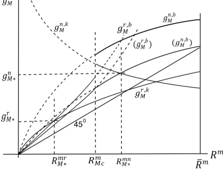
An increase in will raise the slopes of , and , (by shifting up the loci of , and , in a counterclockwise direction). Thus, the loci labeled as
, and , in Figure 2 possess a lower level of than those of , and , . Moreover, ,
and , are independent of . Given these results, Lemma 1 thus implies that, for a given , if the locus of , intersects the locus of , , then the locus of , and , cannot intersect each other. The reverse is also true. Recall that the rationing (non-rationing) equilibrium is determined by the intersection of , and , ( , and , ). Therefore, credit rationing and non-rationing cannot arise simultaneously.
As stated, an increase in raises the slopes of the loci defined by , and
, , while the loci of , and , are independent of . Consequently, the
government spending share plays an important role in determining the equilibrium of the economy. For the illustrative purpose, we define a ∗ such that if ∗ then the loci of , and , intersect each other at . Similarly, define a
̅ such that if ̅ , then the locus of , meets the locus of , at .
Obviously, ̅ ∗. Both ̅ and ∗ are independent of .20 Given these definitions, for a such that ̅ ∗, the locus of , intersects the locus of
, at ∈ , ∗ , implying that there is a unique credit rationing equilibrium.
On the other hand, if ∗ , the loci of , (which is labeled as , in Figure 2) and , cut across each other at ∈ ∗, , so that the unique equilibrium of the economy is characterized by credit non-rationing. We summarize these results in the following proposition.
19
As a result, the loci of , and , ( , and , ) are plotted as dotted lines for
( ) in Figure 2.
20
Note that ∗ 1 . Since is independent of (see
footnote 12), ∗ is also independent of . Moreover, ̅ 1 .
20
Proposition 2 (Equilibrium under Money Financing) If the ratio of government
spending satisfies that ̅ ∗, then there is a unique equilibrium displaying credit rationing. If ∗ , then there is a unique credit non-rationing equilibrium.
The intuition behind Proposition 2 is straightforward. Under money financing, a larger implies that the government must increase seigniorage revenue to a larger extent, which leads to a higher inflation rate and hence a lower . A lower
implies that the type-1 agent is more inclined to mimic the behaviors of type-2 agents. Under the separating equilibrium, the incentive constraint becomes binding and hence type-2 agents are credit rationed. By contrast, if is relatively small, the inflation rate is low and the rate of return from money (and hence deposits) is relatively high. In this case, type-1 agents have no incentive to pretend as type-2 ones, implying that the incentive constraint is not binding and hence type-2 agents can borrow as much as they want.
For future reference, recall that , and , are both greater than . Since the equilibrium of the economy under money financing is the intersection between , , and , , ), the equilibrium growth rates under money financing (i.e., ∗ and ∗) must be always greater than the equilibrium rates of returns for money (i.e., ∗ and ∗).
Before we discuss the equilibrium under tax financing, it is worth noting that there is a nonlinear relationship between inflation and economic growth under money financing. To see this, recall that credit non-rationing (rationing) arises when the inflation rates are relatively low (high), implying that , holds for low levels of inflation (i.e., high levels of ) and , holds for high levels of inflation (i.e., low levels of ). Recall also that the equilibrium is determined by , and , for the non-rationing case and by , and , for rationing case. Then, a further decrease in for ∗, in which the initial ∗ is relatively high, will shift down the locus of , without affecting , . This will leads to an increase in ∗ and a decrease in ∗. Since an increase in ∗ is equivalent to a decrease in the inflation rate, there is a positive correlation between inflation and economic growth
21
for low levels of initial inflation rates. By contrast, a decrease in for ̅
∗, in which the initial levels of the inflation rate are relatively high, will shift down
the locus of , without affecting , . This will lead to an increase in both ∗ and ∗, implying that there is a negative correlation between inflation and economic growth for high levels of initial inflation rates.21 Hence, we have the following result:
Proposition 3. Under money financing, an increase in the inflation rate are
associated with an increase (a decrease) in economic growth for low (high) levels of initial inflation rates.
4.2 Tax Financing
In this case, is equal to so that and hence in eq.(5) of the government budget constraint. Let be the growth rate under tax financing. The condition for the balanced government budget as well as money market equilibrium reduces to .22 On the other hand, the equilibrium
conditions for capital market are still given by eqs.(12) and (13) for the cases of credit rationing and non-rationing. Utilizing eq.(2) with , the growth rates that clear capital market for the cases of credit rationing and non-rationing are given by
, 1 21
and
,
1 , 22 respectively.
Define as the level of under tax financing such that if , then .23 Moreover, we let ∗ ( ∗) and ∗ ( ∗ ) be the equilibrium rates of growth and return from money holdings under credit rationing (non-rationing).
21
Many recent empirical works have discovered this nonlinear relationship. See Hung (2008) for the reference.
22
The government budget constraint can be expressed as . Under tax
financing, and thereby . In other words, (eqs.(15a) and (15b)) is irrelevant for the equilibrium under tax financing.
23
That is, 1 / 1 / . Obviously, is affected by
a change on . Due to this reason, we cannot follow the similar logic of money financing to discuss the equilibrium of the economy.
22
Then, eq.(21) and determine the equilibrium values of ∗, ∗ for the case of credit rationing and eq.(22) as well as determine values of
∗, ∗ for the case of non-rationing. Recall that credit rationing (non-rationing)
arises when . Thus, the equilibrium rate of return from money under credit rationing (non-rationing) must be less (grater) than .
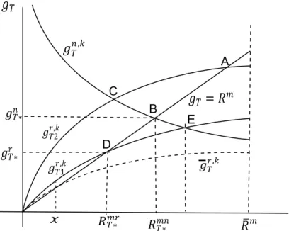
It is clear that , is a concave function of while , is decreasing in . We depict the loci defined by , , , and (a 45-degree line) in Figure 3. The equilibrium of the economy under income-tax financing is determined by the intersection between the 45-degree line and either the locus of , or , .
[Insert Figure 3 here]
Note that both loci of , and , are affected by . For a given value of , the locus of , may intersect the 45 degree line at a that is greater or less than the one at which the locus of , intersects the 45 degree line. We depict each possibility in Figure 3. Consider the first case where, for a given , the locus of , intersects the 45 degree line at Point D while the locus of , intersects the 45 degree line at Point B (the locus of , is labeled as , in Figure 3). Recall that credit is rationing (non-rationing) arises when the equilibrium level of is less
(greater) than . Moreover, when , (and hence , , ).
Thus, is located at point E. Obviously, under the rationing equilibrium ∗ (at point D) is less than (at point E); hence, the equilibrium of credit rationing is viable. On the other hand, at point B where , intersects the 45 degree line, ∗ is less than . This implies that incentive constraint will bind when ∗ .24 Since the equilibrium of non-rationing arises when , credit non-rationing is not the equilibrium in this case.
Consider the second case where the locus of , intersects the 45 degree line at Point A (the locus of , is labeled as , in Figure 3) while the locus of , still intersects the 45 degree line at Point B. Note that the critical value of in this case is located at Point C. Following the similar logic, it is clear that credit is
24
Since ∗ is less than (so that type-2 agent will borrow a larger amount), the incentive
23
non-rationing in equilibrium because the value of at Point B is greater than that at Point C.25
Note that in the first case , intersects the 45 degree line at a (i.e., ∗ ) that is less than the one at which , intersects the 45 degree line (i.e., ∗ of point B). On the other hand, in the second case , intersects the 45 degree line at a
(point A) that is greater than the one at which , intersects the 45 degree line
(i.e., ∗ of point B). Note that ∗ 1 / and ∗
1 . As a result, credit is rationing (non-rationing) in the first (second) case
where ∗ ∗ . In other words, if ∗ ≡ 1 / / , then
∗ ∗ ; and thereby credit is rationing (non-rationing).
Note that if is too large so that the locus defined by , is like the dotted line labeled with ̅ , in Figure 3, then the locus defined by , intersects the 45-degree line at . Since the equilibrium must be greater than , there is no equilibrium in this case. Define a ̅ , ̅ ∗ such that the locus
defined by , cuts across the 45-degree line at if ̅ .26 Then, we have the following proposition.
Proposition 4. Under tax financing, if ̅ ∗, then credit is rationing in
equilibrium; if ∗ , then credit is non-rationing.
The intuition of this proposition is also clear. Under tax financing, the ratio of government spending is equal to the tax rate. A higher (and hence a higher ) leads to a lower after-tax wage rate. This will exacerbate the problem of informational imperfection by inducing type-1 agents to mimic type-2 ones, instead of working for the after-tax wage. As a result, the incentive constraint becomes binding and credit is rationing.
Note that the inflation-growth relationship is linear under tax financing. To see this, note that an increase in shifts both loci of , and , down without affecting the 45 degree line and rationing (non-rationing) arises for high (low) levels of inflation rates. Thus, if the initial inflation rates are low, a further increase in ,
25
Credit rationing is not the equilibrium in this case because the value of at Point A (the rationing equilibrium) is greater than that at Point C (the critical value).
24
which shifts down , without influencing the 45 degree line, leads a decrease in both ∗ and ∗ , implying that there is negative correlation between inflation and economic growth. On the other hand, if the initial inflation rates are relatively high, a further increase in , which shifts down , without influencing the 45 degree line, again leads to a decrease in both ∗ and ∗ . Hence, we have the following result:
Proposition 5. Regardless the initial level of the inflation rate, the
inflation-growth relationship is always negative under tax financing.
Before comparing the equilibrium economic growth, inflation, and social welfare, it is worth noting that our model may provide theoretical explanations to recent empirical studies on the inflation-growth correlations. Since the work of Fischer (1993), a large body of literature [Bruno and Easterly, 1998; Ghosh and Phillips, 1998; Khan and Senhadji, 2001; Burdekin et al., 2004] has discovered a nonlinear correlation between inflation and economic growth. In particular, these studies reach a consensus that an increase in the inflation unambiguously leads to a decrease in economic growth for high levels of initial inflation rates. For low levels of initial inflation rates, an increase in the inflation rate may lead to a decrease, an increase, or have no significant effect on economic growth.
Recall that credit rationing (non-rationing) arises for high (low) levels of initial inflation rates. According to Propositions 3 and 5, an increase in the inflation rate always leads to a decrease in economic growth for high levels of initial inflation rates (i.e., under the rationing equilibrium), regardless how the government finances its spending. However, for low levels of initial inflation rates (i.e., under the
non-rationing equilibrium), an increase in the inflation rate leads to an increase (a decrease) under money (tax) financing. Accordingly, if we pool all countries (who may finance their expenditure by printing money or levying tax) together, then we may reach a conclusion that an increase in the inflation rate may lead to an increase, a decrease, or have no significant effect on economic growth, depending on the number of countries that utilize tax or money financing in the sample.
25
Recall that, for a given , credit is rationing (non-rationing) if ∗ ( ∗ ) under tax financing. Similarly, under money financing credit rationing (non-rationing) if ∗ ( ∗ ). To simplify our analysis, we report the two cases:
̅ , ̅ ∗, ∗ and ∗, ∗ .27
The case of ̅ , ̅ ∗, ∗ indicates that the equilibrium displays credit
rationing no matter how the government finances its spending. Similarly, the case of
∗, ∗ implies that the equilibrium exhibits non-rationing regardless
whether the government finances its spending by money or tax financing.
5.1 Comparing Output Growth
Case 1. Credit Rationing: ̅ , ̅ ∗, ∗
We depict the loci defined by , , , and , with the 45-degree line in Figure 4. A comparison between eqs. (18) and (21) reveals that for a given the locus of , is higher than that of , , as is depicted in Figure 4. Moreover, the locus of , is higher than that of the 45-degree line. Recall also that equilibrium rate of growth under tax financing ∗ is determined by the intersection of , and the 45-degree line (Point J in Figure 4); hence,28
∗
1 / /
∗ , 23
where ∗ is the inverse of the equilibrium inflation rate under tax financing.
[Insert Figure 4 here]
On the other hand, ∗ is determined by the intersection of , and , . To compare ∗ with ∗ we first substitute ∗ into , to obtain the
corresponding (which is denoted as in Figure 4). Substituting this into
, (i.e., eq.(17)), we derive the corresponding growth rate under eq. (17) (denoted
as in Figure 4). Clearly, if is greater than ∗ (such as point G in Figure 4), then the loci of , and , must intersect each other at the growth rate ∗ that is less than ∗. On the other hand, if the locus of , is like the one labeled as
27
It is obvious that ∗ may be greater or less than ∗. Thus, depending on whether the spending is financed by printing money or taxation, an economy with a given may be under rationing or non-rationing regimes. We compare the growth rate and the inflation rate for this situation in Appendix B (not intended for publication).
28
Note that the growth rate is equal to under the 45-degree line. Substituting ∗ into
26
, in Figure 4, then (which is equal to in Figure 4) is less than
∗. In this
case, it is clear that ∗ (denoted as ∗ in Figure 4) must be greater than ∗.
Note that 1 / / . Hence, ∗ ∗ if
∗
1 / /
1 1 / /
1 1 / 1 / / 1
1. 24
After some manipulations, it can be found that ∗/ 1 is always satisfied for any 0. Hence, we conclude that ∗ ∗ for any , ̅ , ̅
∗, ∗ . We summarize this result in the following proposition.
Proposition 6. For a given where ̅ , ̅ ∗, ∗ , the
equilibrium growth rate of tax financing is greater than that of money financing.
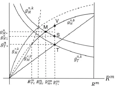
Case 2. ∗, ∗
Regardless of financing method, credit is non-rationing in this case.Recall that the equilibrium growth rate in the non-rationing case is determined by the intersection of
, and the 45-degree line under tax financing. This implies that the equilibrium
growth rate is located at the 45-degree line, as depicted in Figure 5.29 On the other hand, the equilibrium growth rate under money financing is determined by the intersection between , and , . A comparison between eqs. (20) and (22) reveals that the locus of , is higher than that of , for any given and . Moreover, for any given the growth rate obtained from , is always greater than , implying that the locus defined by , is always higher than the
45-degree line. This further implies that the growth rate under money financing (the intersection of , and , ) is always greater than that under tax financing (the intersection between , and the 45-degree line).30 The following proposition summarizes our result.
[Insert Figure 5 here.]
29
Recall that 1 / 1 / and 1
1 1 1/ 2 . Obviously, as depicted in Figure 5.
30
In Figure 5, ∗ and ∗ are the equilibrium growth rates while ∗ and ∗ are the rates
27
Proposition 7. For any given , min ∗, ∗ , the equilibrium growth rate of
money financing is greater than that of tax financing.
5.2 Comparing the Inflation Rate
Again, we compare the equilibrium inflation rate for the rationing equilibrium and non-rationing equilibrium.
Case 1. Credit Rationing
The equilibrium for tax financing is denoted as ∗ (point J in Figure 4). Alternatively, for given parameters, we depict two possibilities for the equilibrium
under money financing: one is less than ∗ (denoted as ∗) and the other one is greater than ∗ (denoted as ∗ in Figure 4). Since the equilibrium
under money financing is determined by the intersection of , and , . Results of Lemma 1 imply that the equilibrium under money financing is lower than that of tax financing if the growth rate obtained from , is greater than that obtained from
, when
∗ (see Figure 4).31 Substituting ∗ from eq. (23) into ,
and , , the condition that money financing leads to a lower rate of return from money holdings can be expressed as
1 / / 1 1 / / /
1 1 1 1 / / /
1
.
The sufficient condition for the above inequality is 1 1 , which
always holds since 1 1 1 / 1 . Thus, we have the
following result:
Proposition 8. For any , ̅ , ̅ ∗, ∗ , money financing
results in a higher inflation rate than tax financing.
31
In Figure 4, when ∗, then the growth rate derived from the locus of , is greater
than that derived from the locus of , . By contrast, when ∗, then the growth rate derived
from the locus of , (point X in Figure 4) is less than that derived from the locus of , (point H). In the former case, the equilibrium under money financing is less than ∗, while the reverse is
28 Case 2. Non-rationing
Following the similar logic of Proposition 6, the equilibrium under money financing is less than that under tax financing if the growth rate of the locus , (Point V in Figure 5) is greater than that of the locus , (Point S) when
∗ . Substituting ∗ into , and , , we see that the resulting growth rate of
the locus , is greater than that of the locus , if
1 1 1
1
1 1 1 1 .
Since Assumption A2 implies that 1 1 , a
sufficient condition for the above inequality is 1 1, which always holds for 1 0. Hence, we have the following preposition.
Proposition 9. For any , min ∗, ∗ , the inflation rate under money
financing is greater than that under tax financing.
The intuitions of Propositions 6 and 7 are straightforward. For a given , money financing requires the government to print more money (than tax financing), regardless whether the equilibrium displays credit rationing or non-rationing. Printing more money leads to a higher inflation so that money financing yields a higher inflation rate than tax financing. With respect to economic growth, both money financing and tax financing under non-rationing equilibrium alleviate the problem of asymmetric information and hence enable type-2 agents to borrow more.32
Proposition 7 implies that the amount borrowed by a type-2 agent (i.e., ) under money financing is higher than that under tax financing for a given , with
min ∗, ∗ . This leads to a higher rate of economic growth under money
financing compared with tax financing.
5.3 Comparing the Welfare
32
29
The analysis proceeded so far indicates that ∗ ∗ ∗ ∗ in the rationing equilibrium and ∗ ∗ ∗ ∗ in the non-rationing
equilibrium. Given these results, we now compare the welfare of type-1 and type-2 agents under tax financing and money financing.
At the initial period 0 , there are type-1 old agents and each of them is endowed with units of capital. These agents utilize the capital and hire young type-1 agents to produce output, which is taxed at a rate of (under tax financing). As a result, the after-tax wage income for each young type-1 agent is 1
while the after-tax capital income for each (initial) old type-1 agent is 1 . Each young type-1 agent lends 1 / units to a type-2 young agent and each type-2 agent produces units of time 1 capital.As a result, each old type-1 agent at 1 receives 1 / units of capital. The old type-1 agent rents this capital to firms and obtains the after-tax return given as 1 . Since the loan rate is equal to ∗ , it is clear that the old type-2 agent at 1 will
receive 1 1 ∗ / .
Denote ∗ as well as ∗ as the equilibrium growth rate and rate of returns from money. Then, the above scenario implies that the welfare of type-1 agents for all generations under the balanced growth path can be expressed as33
1 1 1 ∗ 1 1 1 ∗ ⋯ 1 ∗ 1 ∗ ⋯ 1 1 ∗ ∗ under tax inancing 1 ∗ ∗ under money inancing, 25
where is the constant discounted rate for each period. We assume that ∗, , ,
is less than to ensure the boundedness of the utility. Obviously, for given
33
We follow the standard practice by ignoring the initial old type-1 agents' utility. Note that each agent cares only old-age consumption. As a result, the utility of the first generation (born at time 0) is discounted at the rate , because the government evaluates the social welfare from time 0. Note that the population of type-1 agent is equal to .
30
parameters tax financing yields a higher (lower) welfare level for type-1 agents than money financing if
1 ∗
∗
∗
∗. 26
Recall that, under the rationing equilibrium, tax financing yields a higher rate of economic growth and a lower rate of inflation compared with money financing. However, this does not guarantee that tax financing yields a higher level of welfare to type-1 agents than money financing, as the tax rate (which is equal to ) appears in the welfare function under tax financing. Note that ∗ . Hence, if 1 ∗ ∗ (a sufficient condition) for a given in the rationing equilibrium, we can be sure that tax financing yields a higher level of welfare to type-1 agents than money financing. To compare 1 ∗ with ∗, we depict Figure 6.
[Insert Figure 6 here]
Recall that ∗ is determined by , and the 45 degree line (hence,
∗ 1 / . Then, multiplying ∗ with 1 and
substituting it into , (point Z in Figure 6) and , (point U in Figure 6), Lemma 1 implies that 1 ∗ is greater than ∗ if the resulting , is greater than
, ; i.e., , , ∗ 1 ∗ 1 1 ∗ 1 1 1 1 ∗ 1 ∗ 1.
After some manipulations, the above equation reduces to .
1 1 ∗ 1 1 1 1 ∗ 1 1 , or σ 1 σ 1 1 ∗ ,
31
which always holds for 0. Hence, under the rationing equilibrium tax financing yields a higher level of welfare to type-1 agents than money financing. Note that this result confirms that 1 ∗ ∗.
In the case of the non-rationing equilibrium, recall that ∗ ∗ ∗
∗. From this, we cannot directly infer the relative merits of government financing
from the perspective of type-1 agents’ welfare. Nevertheless, we can derive a condition showing that money financing may be better than tax financing under the non-rationing equilibrium. To see this, eq. (26) leads to the following sufficient condition under which money financing yields a higher level of welfare for type-1 agents:34 ∗ ∗ ∗ ∗ . Rewrite the above equation as
∗
1 ∗
∗
1 ∗,
which, after some manipulations, is equivalent to
1 ∗
∗
∗ ∗ ≡ ∗. 27
Since ∗ ∗ ∗ ∗, ∗ 1. Eq. (27) is quite intuitive. From eqs. (25) and (26), the importance of economic growth in affecting the welfare of type-1 agents depends positively on the discount rate. In other words, if the discount rate is not too small, economic growth is more important on the welfare compared with the rate of returns from money. Since ∗ ∗ ∗ ∗, it is then clear that if the discount rate is not too small, money financing yields a higher level of welfare for type-1 agents.
The welfare of type-2 agents for all generations is given by35
34
This is a sufficient condition because ∗
∗
∗ ∗. 35
Note that and (as well as ) in all periods are in terms of per type-l agent. As a result, the utility of all
type-2 agents (total population is equal to 1 is also expressed in terms of per type-1 agent, implying that the
32
1 ∞
1
1 ∗
1 ∗ ⋯ 28 where is equal to ( under the rationing (non-rationing) equilibrium. From eq. (11), the above equation can be rewritten as
1 ∗ 1 1 ∗ ∗ 1 1 ∗ ⋯,
where ∗ has been substituted. Under the rationing equilibrium,
1 1 ∗ / and ∗ ∗. Then, the above equation
becomes 1 ∗ ∗ 1 1 1 1 ∗ 1 ∗ ∗ 1 1 ∗ tax inancing ∗ ∗ 1 1 ∗ money inancing, Since ∗ ∗ ∗ ∗ under the rationing equilibrium, tax financing
yields a higher level of welfare to type-2 agents if
∗ ∗ 1 ∗ ∗ ∗ ∗ 1 1 ∗ 1 1 ∗ . 29
33
Recall also that 1 ∗ ∗ under the rationing equilibrium. Thus, a
sufficient condition that leads to a better tax financing than money financing (from the perspective of type-2 agents’ welfare) is given as
∗ ∗ ∗ ∗ 1 1 ∗ 1 1 ∗ ≡ .
Note that 1, since ∗ ∗ ∗ ∗. After some manipulations, the above equation implies that
1
∗ ∗ ≡ ∗.
Note that ∗ 1. Thus, if the discount rate is not too small, tax financing under the rationing equilibrium yields a higher level of welfare for type-2 agents than money financing.
Substituting into eq. (26), we have
1 1 1 1 ∗ ∗ 1 ∗ ∗ ∗ ∗ .
The above equation shows that the welfare of type-2 agents is increasing in economic growth and decreasing in the rate of returns from money. Recall that ∗
∗ ∗ ∗ under the non-rationing equilibrium. Thus, in the non-rationing
equilibrium money financing always leads to a higher level of welfare for type-2 agents than tax financing. We summarize our analysis in the following proposition:
The social welfare function for the economy as a whole is the summation of the welfare functions of type-1 and type-2 agents. By assuming that ∗, ∗ , we have the following result:
Proposition 10. Under the rationing equilibrium, tax financing yields a higher level
of the social welfare than money financing. On the contrary, under the non-rationing equilibrium money financing yield a higher level of the social welfare than tax financing.