國立交通大學
電子工程學系 電子研究所碩士班
碩 士 論 文
聯合訊源通道編碼技術用於
無線近身網路之心電訊號壓縮
Joint Source-Channel Coding for Electrocardiogram
(ECG) Compression on Wireless Body Area Networks
學生:莊憲榮
指導教授:張錫嘉教授
國立交通大學
電子工程學系 電子研究所碩士班
碩 士 論 文
聯合訊源通道編碼技術用於
無線近身網路之心電訊號壓縮
Joint Source-Channel Coding for Electrocardiogram
(ECG) Compression on Wireless Body Area Networks
學生:莊憲榮
指導教授:張錫嘉教授
聯合訊源通道編碼技術用於無線近身網路之心電訊號壓縮
Joint Source-Channel Coding for Electrocardiogram (ECG) Compression
on Wireless Body Area Networks
研 究 生:莊憲榮 Student:Hsien-Jung Chuang 指導教授:張錫嘉 博士 Advisor:Dr. Hsie-Chia Chang
國 立 交 通 大 學
電子工程學系 電子研究所碩士班 碩 士 論 文
A Thesis
Submitted to Department of Electronics Engineering & Institute of Electronics
College of Electrical and Computer Engineering National Chiao-Tung University
In Partial Fulfillment of the Requirements For the Degree of Master of Science
In
Electronics Engineering
Sep. 2013
Hsinchu, Taiwan, Republic of China
聯合訊源通道編碼技術用於
無線近身網路之心電訊號壓縮
學生:莊憲榮
指導教授:張錫嘉 教授
國立交通大學
電子工程學系 電子研究所碩士班
摘 要
在無線近身網路中,心電訊號壓縮是一項用來監測心臟相關疾病的重要技 術。由於以往的心電壓縮技術著重於高壓縮率以及高速傳輸,在編碼端有比較高 的複雜度,並不適用於無線近身網路。據此,本論文採用向量量化和索引指定方 法來設計低複雜度的訊號壓縮器。此外,我們在解碼端考慮了通道效應,設計了 迴旋編碼器提供資料保護並採用聯合訊源通道解碼的架構,搭配所提新的事前機 率初始方法,不但達到良好的訊號重建品質,也提升了解碼速度。在 MIT-BIH 資料庫模擬結果,相較於其他心電傳輸技術,本論文所採用的架構能以較低複雜 度之壓縮器,搭配迴旋碼達成良好重建品質並提高 1.5 倍收斂速度。Joint Source-Channel Coding for Electrocardiogram
(ECG) Compression on Wireless Body Area Networks
Student:Hsien-Jung Chuang
Advisor:Dr. Hsie-Chia Chang
Department of Electronics Engineering
Institute of Electronics
National Chiao Tung University
ABSTRACT
A wireless body area network (WBAN) for ECG compression is a promising approach for monitoring cardiac disease. Based on percentage root-mean-square difference (PRD) requirements, many ECG compression techniques have been introduced to achieve high compression ratio (CR) but may not be suitable in WBAN due to their higher encoding complexity. In this thesis, the joint source-channel
coding scheme is proposed to not only adopt vector quantization and index
assignment as the ECG compressor, but apply channel decoding technique to ensure robust ECG transmission. Note that the encoder parameters can be modified to obtain better reconstructing ECG signals at fixed CR. In addition, a new a priori
knowledge initialization algorithm is presented to provide 1.5 times converge speed in
contrast to original iterative source-channel decoding algorithm. After simulating with the MIT-BIH arrhythmia database, the results show that the proposed schemes with low encoding complexity has higher reconstruction quality than previous works.
誌 謝
三年的碩班生涯,有了家人以及朋友的陪同,使我能在這條路上走得開心順 利,良好的實驗室環境,最佳的實驗室資源,這些不管在我研究上或者生活上都 扮演著重要腳色。 首先要感謝指導教授張錫嘉老師,提供了研究上的建議,財力上的支援,日 常生活上的關心,及自由的研究環境,讓我在這三年的研究能夠完成。接著要感 謝在業界工作的建青學長,在我實習時總是不吝指教,學長做事情的態度為我做 了最好的楷模,在我研究上,更是常提供一針見血的建議。還有帶我的實驗室學 長振揚,雖然我們研究方向上的不同,學長還是會就研究上的不足,提供實際建 議,有問必答,讓我在通道編碼這領域有更多的了解。最後要謝謝 OCEAN 以及 OASIS 團隊,你們的熱心指點及協助,讓我能在這三年快樂的完成學業。 最後,我要感謝我的家人,謝謝我的爸爸和媽媽,對我的精神鼓勵以及財力 上的支援,讓我能順利完成碩士論文,最後要感謝口試委員,給予我的寶貴意見。 中華民國 一○二年 九月 莊憲榮Contents
1 Introduction 1
1.1 Background . . . 1
1.2 Motivation . . . 2
1.3 Thesis Organization . . . 3
2 Digital communication system 4 2.1 Source Encoder . . . 5
2.2 Channel Encoder . . . 9
2.3 Soft Iterative Decoding . . . 12
2.3.1 Extrinsic Information . . . 13
2.3.2 Exchange of Extrinsic Information . . . 15
2.4 Soft-Output Channel Decoding . . . 18
2.5 Softbit Source Decoding . . . 22
3 Joint Source-Channel Coding Scheme 26 3.1 System Overview . . . 27
3.2 Vector Quantizer with LBG Algorithm . . . 29
3.3 Index Assignment with Pseudo-Gray Code . . . 32
3.4 Iterative Source-Channel Decoding (ISCD) Algorithm . . . 37
3.4.1 BCJR Algorithm for Channel Decoding . . . 39
3.4.2 Softbit Source Decoding . . . 46
3.5 Proposed A Priori Knowledge Initialization . . . 48
4 Simulation Results 51 4.1 Conventional ISCD Performance . . . 52
4.2 Different Encoder Configurations Analysis . . . 54
4.2.1 Vector Dimension . . . 54
4.2.2 Index Assignment . . . 56
4.2.3 Channel Encoder . . . 57
4.3 Proposed ISCD Performance . . . 58
4.4 Comparison of Different ECG Compression Techniques . . . 60
5 Conclusion and Future Work 62 5.1 Conclusion . . . 62
5.2 Future Work . . . 63
List of Figures
1.1 Wireless body area network system . . . 3
2.1 Communication system diagram . . . 4
2.2 Source encoding flow . . . 5
2.3 Quantization flow . . . 6
2.4 Block diagram of recursive convolutional encoder . . . 10
2.5 Block diagram of two equivalent (2,1,2) convolutional codes . . . 11
2.6 State diagram of the (2,1,2) recursive systematic convolutional codes . . . 12
2.7 Graph representation of the extrinsic and the intrinsic probabilities . . . 13
2.8 Graph representation of the extrinsic exchanging between two vertices . . . 15
2.9 The bipartite graph for the (7,4) Hamming code . . . 19
2.10 Conventional parameter decoding by hard decision . . . 22
2.11 Softbit source decoding by parameter estimation . . . 23
3.1 Block diagram of the transmitter . . . 27
3.2 Block diagram of the receiver . . . 29
3.3 1-bit vector quantizer design with LBG algorithm . . . 33
3.4 2-bit vector quantizer design with LBG algorithm . . . 33
3.5 Block diagram of VQ on noisy channel . . . 34
3.6 Flow chart of the binary switch algorithm . . . 38
4.1 Parameter SNR of conventional ISCD . . . 53
4.2 γ of conventional ISCD . . . . 54
4.3 Comparison of different vector dimensions . . . 55
4.4 Comparison of different index assignments . . . 56
4.5 Comparison of different RSCs . . . 58
List of Tables
2.1 Quantization Table . . . 7
2.2 Index assignment table . . . 9
4.1 Parameters Configuration 1 . . . 52
4.2 Parameters Configuration 2 . . . 55
4.3 Parameters Configuration 3 . . . 56
4.4 Parameters Configuration 4 . . . 58
4.5 Parameters Configuration 5 . . . 59
Chapter 1
Introduction
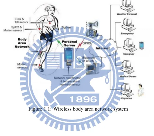
For elderly people and those at the risk of various heart diseases, medical service providers invest in remote ECG monitoring systems to take good care of patients by tracking of their health states. Fig.1.1 [1] shows a wireless body area network (WBAN) system for ECG trans-mission. The system, which includes sensors and a wireless transmitter, needs to be as small as possible for better user experience. However, these kind of remote systems are difficult to design. There are many restrictions like power consumption and limited resources. Since a large percent of power is consumed up by the transmitter, so we conduct a research to reduce the transmitted data size as well as ensure data correctness over noisy wireless channels. There-fore, the compressor and the protector are added to the transmit side for the data compression and correction. In this thesis, we investigate low complexity algorithms to achieve better com-pression and protection. Simulation results will be provided to support our findings.
1.1
Background
Generally, data compression can be categorized into loss and lossless methods. For ECG data compression, the loss type has been applied for high compression ratio (CR) and pre-serve clinical information. ECG data compression can be divided into three groups. The first groups are direct data compression. They base their detection of redundancies on analysis in time domain. Examples include turning point (TP) [2], amplitude zone time epoch coding
(AZTEC) [3], coordinate reduction time encoding system (CORTES) [4], the delta algorithm and the Fan algorithm [5]. The second groups are transformation methods [6]. They convert the time domain signal to the frequency or other domains. They mainly utilize the spectral distribution analysis for redundancies. Example include Fourier transform, Karhunen-Loeve transform (KLT), Walsh transform, and the discrete cosine transform (DCT), and the wavelet transform [7]. The third groups are parameter extraction techniques. They extract the char-acteristic and parameters of the signal. The extracted parameters are subsequently used for classification based on a priori knowledge of the signal. Examples include the peak picking method [8], the linear prediction method [9], the neural network method [10].
1.2
Motivation
Although there already exists many compression techniques, due to the application of WBAN application, which means limited electronic resources, only simple computations can be done. Additionally, these techniques have been introduced purely achieve the high CR on some PRD requirement. However, in WBAN application, the comprehensive lossy compression on noisy channel should be considered.
In this thesis, we introduce a joint source-channel coding methodology to enchance the compression quality with error correctablity in WBAN. The approach is based on the vector quantization. Under different channel conditions, the resulting vector dimensions are used re-spectively to gain a decoding performance. Vector quantization and convolutional coding plus some simple puncturing in the transmitter, may have the chance to meet the limitation of com-putation complexity for ECG compression. Furthermore, we proposed an efficient algorithm in the decoding procedure. The algorithm provides more accurate source information in bad channel environment and improves the convergence in ISCD.
1.3
Thesis Organization
This thesis is organized as follows. In Chapter 2, we introduce the modern digital systems and discuss several source and channel coding techniques. Chapter 3 will first identify the sys-tem notations. Then, the algorithms of each units and the proposed initialization are provided. Chapter 4 gives the simulation results and the comparison with other related works. Finally, conclusions and future works are given in Chapter 5.
Chapter 2
Digital communication system
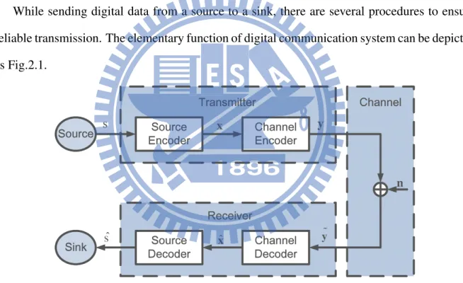
While sending digital data from a source to a sink, there are several procedures to ensure reliable transmission. The elementary function of digital communication system can be depicted as Fig.2.1.
Figure 2.1: Five elements (gray unit) of digital communication system
The information source generates a signal s. The transmitter encodes a time segment of s by a code sequence y. Generally, the goal of the encoder mapping is to minimize the undesirable effects of channel noise on the signal. The actual procedure of transmitter can be separate into two parts, called source and channel encoding. The source encoder performs the compression by using a code sequence x to represent s. The channel encoder inserts some artificial redun-dancy, known as parity check symbols, to minimize the transmission error. Some errors could
be detected and/or corrected. The code sequence x is expanded to a code sequence y. The third element is transmission channel. The noise sequence n adds to y. The receiver exploits the received sequence ˜yin order to recover the source s. The reconstructed signal ˆs is sent to the
sink.
2.1
Source Encoder
The goal of source coding is to remove redundancy from source, also known as data com-pression or bit-rate reduction. The ECG signal is continuous in time and magnitude. The digi-talize and quantize process adds some artificial noise to the ECG signal. However, the distortion of reconstruction signal is tolerably accepted.
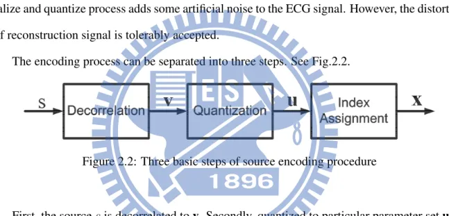
The encoding process can be separated into three steps. See Fig.2.2.
Figure 2.2: Three basic steps of source encoding procedure
First, the source s is decorrelated to v. Secondly, quantized to particular parameter set u, in the quantizer codebook U (u∈ U). Finally, the quantized set u is one-to-one mapping into the set of bit pattern x.
Decorrelation is the main part to remove redundancy of the source data. This process is generally lossless and invertible. In order to decorrelate the source signal, there are two types of the signal correlation.
• Autocorrelation
Autocorrelation is the similarity between a given signal and its lagged version. In the other words, the correlation with a signal between two different time series is autocorre-lation. It is also referred to as lagged correlation or serial correautocorre-lation. The autocorrelation of white noise signal will have a peak at the origin and will be zero otherwise. The
au-tocorrelation of periodic signal will have a peak at the origin and repeat with the same period.
• Cross-correlation
Cross-correlation is the similarity between two different signals. The decorrelation al-gorithm must be applied to multiple recordings of the same signal generated in different transmitting channels, such as the multichannel ECG signal. The noise and distortion in different channels are independent, but they have the same source statistic distribution. Distributed source coding(DSC) [11] is a way to solve the cross-correlation problem, and it is used in multimedia or video compression. One of the DSC properties is encoder complexity shifted to decoder.
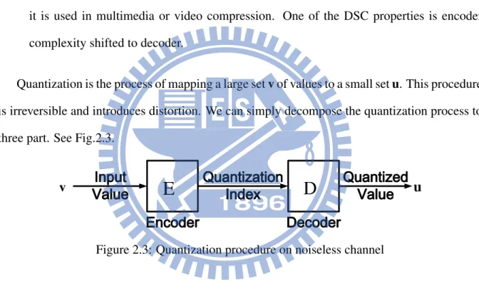
Quantization is the process of mapping a large set v of values to a small set u. This procedure is irreversible and introduces distortion. We can simply decompose the quantization process to three part. See Fig.2.3.
Figure 2.3: Quantization procedure on noiseless channel
Quantization usually involves encoder and decoder. An encoding or forward quantization part is represented by ”E”, which maps an input value to quantization index. And a decoder or backward quantization part is represented by ”D”, which maps the index to quantization value. Two basic type of quantization will be discussed below.
• Scalar quantization
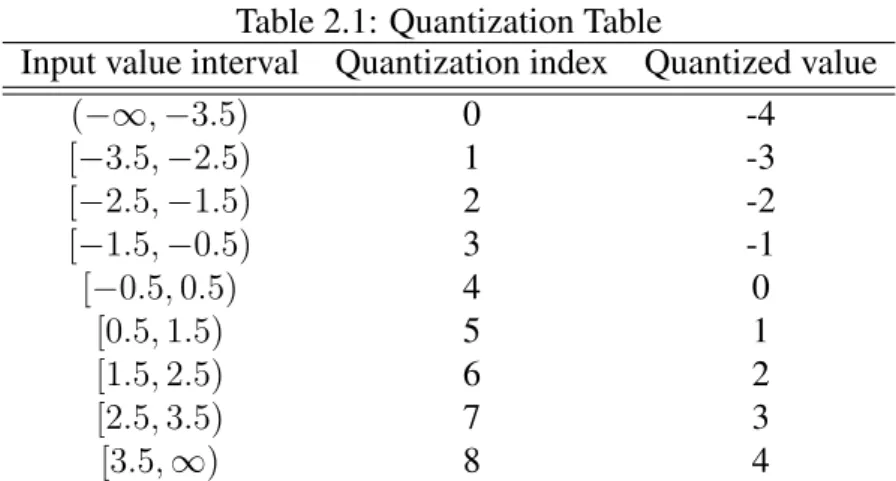
Scalar quantization is the most common type of quantization. It is a process to map a scalar input value to output value output. Table 2.1 shows an example of uniform scalar quantization.
Table 2.1: Quantization Table
Input value interval Quantization index Quantized value (−∞, −3.5) 0 -4 [−3.5, −2.5) 1 -3 [−2.5, −1.5) 2 -2 [−1.5, −0.5) 3 -1 [−0.5, 0.5) 4 0 [0.5, 1.5) 5 1 [1.5, 2.5) 6 2 [2.5, 3.5) 7 3 [3.5,∞) 8 4
The quantization maps an infinite range of values into nine integers, which needs 4 bit to represent. We call this quantizer a 4-bit scalar quantizer. The uniform quantization means the quantized values are equally spaced. When an analog signal is uniformly sampled and uniformly quantized, the resulting digital representation is called pulse-code modulation. It is commonly used in digital communication systems, such as speech, audio, and video. The opposite of uniform quantization is nonuniform quantization. The origin of nonunform quantization aim at reducing the quantization error. The nonuniform quantizer design is an optimization problem: Finding a good quantization that minimized the quantization error. A good approach is Lloyd-Max algorithm [12] [13]. The optimal quantizer must satisfy the centroid condition and nearest neighbour condition proposed by [12] [13]. So, the optimal quantizer is also referred to as Lloyd-Max quantizer.
• Vector quantization
Vector quantization design algorithm is first proposed by Linde, Buzo, and Gray(LBG) [14]. The LBG algorithm is often used to design the codebook in vector quantization. This algorithm is also referred to k-means algorithm or generalized Lloyd’s algorithm. Vector quantization is originally used for lossy compression. It encodes values form multidimentional vector space to a finite set of vector. The index of the vector is sent instead of the quantized values, this achieves more compression. Vector quantization is also used to lossy data correlation. If some dimensions are losses, it can be recovered by available dimensions through the nearest group. Compared with scalar quantization,
vector quantization results in lower distortion when the source is correlate, and more flexibility in bit rate when the source is no dependency. But the codebook design of vector quantization requires large computation complexity, and it is closely related to compression quality.
Index assignment is the final step of source encoding the quantization index to a particular bit pattern. The following three index assignment is important for iterative source-channel decoding and suitable for scalar quantization.
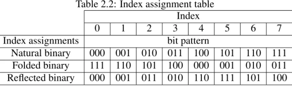
• Natural binary
If the bit pattern encodes the quantization indexes to binary patterns in increasing order, the mapping is called natural binary code. The leftest bit is most significant bit which usually cause high distortion due to the channel noise. The rightest bit is least significant bit causes small distortion.
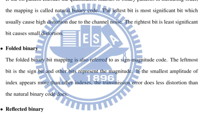
• Folded binary
The folded binary bit mapping is also referred to as sign-magnitude code. The leftmost bit is the sign bit and other bits represent the magnitude. If the smallest amplitude of index appears more than other indexes, the transmission error does less distortion than the natural binary code does.
• Reflected binary
The reflected binary bit mapping is also known as Gray code. The term reflected binary code is first introduced by Frank Gray in 1947 [15]. Gray code maps every two successive quantization indexes to bit streams with one differ bit. When single transmission error occurs more than multiple transmission errors, Gray code results in smaller distortion than other mappings.
Table 2.2 shows different index assignments after 8-level quantization.
The index assignment techniques mentioned above are commonly used in digital transmis-sion systems. However, these techniques are restricted to scalar quantization. In vector quanti-zation, we do not know which quantization indexes are successive or rearrange these indexes in
Table 2.2: Index assignment table Index
0 1 2 3 4 5 6 7
Index assignments bit pattern
Natural binary 000 001 010 011 100 101 110 111 Folded binary 111 110 101 100 000 001 010 011 Reflected binary 000 001 011 010 110 111 101 100
increasing order. Pseudo Gray code is first proposed by Kenneth Zeger and Allen Gersho [16], which minimizes the distortion operated on noisy channel for vector quantization. The further discussion about pseudo Gray code will be listed in chap 3.
2.2
Channel Encoder
Channel coding adds some artificial redundancy to the information bits after source encod-ing. The redundancy helps the receiver to correct the error caused by channel noise. Channel coding can detect and correct transmission errors. There are two types of channel codes.
• Linear block codes
An (n,k) binary block code is a one-to-one mapping of k bit information sequence x and n bit codeword y. A binary block code is linear if and only if the module-2 sum of two codewords is also a codeword. The encoding procedure of linear block code can be realized in terms of matrix operation y = xG, where x, the information sequence, is a k bit row vector, and G, the generator matrix, is a k by n matrix. Every generator matrix G can be converted to a generator matrix in row-echelon form. Then, by column operations, every generator matrix can be further converted to a generator matrix G′ denoting as [I P] which is concatenated by a k by k identity I and a k by n− k matrix P. We call this the systematic form of a generator matrix, and we call the code is systematic if the information sequence x itself is part of codeword, y′ = xG′ = (x, r). The redundant bits r contains n−k bits, known as parity check bits. Different coefficient setting of G generate different linear block codes. Famous examples of linear block codes are Hamming code, Reed-Solomon code, Hadamard code, and LDPC code.
• Convolutional codes
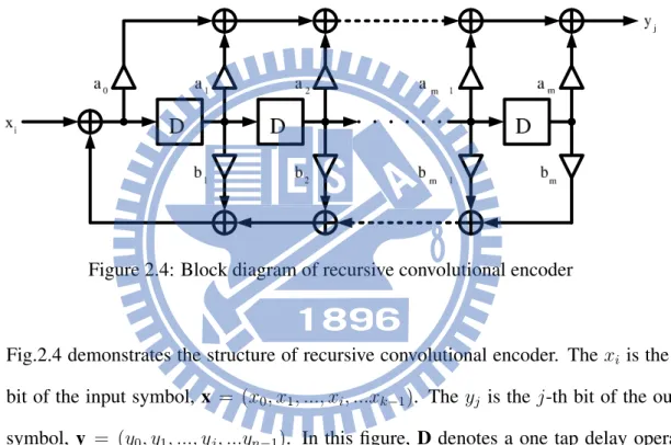
Convolutional codes was first proposed by Elias [17] in 1955. Compared to linear block codes, the convolutional codes contains memories. The encoder saves the previous in-formation symbols in several memory elements. Combining both previous symbols and current symbol to generate the convolutional codewords. For an (n,k,m) convolutional code, every k-tuple information symbol will be encoded to an n-tuple codeword symbol by the encoder with memory order m. The error correction performance is determined by the memory order m and the code rate R = k/n.
Figure 2.4: Block diagram of recursive convolutional encoder
Fig.2.4 demonstrates the structure of recursive convolutional encoder. The xi is the i-th
bit of the input symbol, x = (x0, x1, ..., xi, ...xk−1). The yj is the j-th bit of the output
symbol, y = (y0, y1, ..., yj, ...yn−1). In this figure, D denotes a one tap delay operator.
Besides, a0 ∼ am and b1 ∼ bm determine the connections of circuit, each of them is
either 0 or 1. We can use a fractional function gi,j(D) as (2.1) to express this encoder
realization.
gi,j(D) =
a0+ a1D +· · · + amDm
1 + b1D + b2D2+· · · + bmDm
(2.1)
Similar to linear block codes, the entire set of k× n generator polynomials gij(D) can be
G(D) = g0,0(D) g0,1(D) · · · g0,n−1(D) g1,0(D) g1,1(D) · · · g1,n−1(D) .. . ... . .. ... gk−1,0(D) gk−1,1(D) · · · gk−1,n−1(D) (2.2)
Moreover apply some matrix operation on the generator matrix G(D) generally gets a systematic form G′(D). Here we use the (2,1,2) convolutional encoder as an example. The Fig.2.5(a) is a convolutional encoder with G(D) = [1 + D + D2, 1 + D2]. The
Fig. 2.5(b) is the equivalent recursive systematic convolutional encoder with G′(D) = [1,1+D+D1+D22].
(a) Non-recursive convolutional code (b) Recursive systematic convolutional code
Figure 2.5: Block diagram of two equivalent (2,1,2) convolutional codes
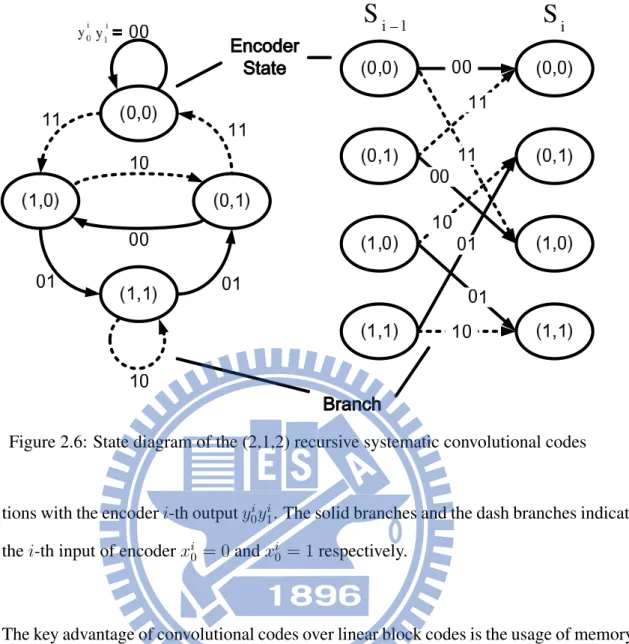
Besides the matrix description of convolutional codes, a convolutional codes can be de-scribed in a state diagram. The state diagram comprises encoder states and state transition. The states are the contents of all delay elements. If the the memory order of encoder is
m, the total number of states is 2m. The state transition is caused by the input data. Here we use the (2,1,2) encoder (Fig.2.5(b)) as an example.
The previous content of memory elements are represented as di0−1 and di1−1. All com-binations of (di−10 ,di−11 ) represent previous encoder states noted as Si−1. The ellipses of
transi-Figure 2.6: State diagram of the (2,1,2) recursive systematic convolutional codes
tions with the encoder i-th output y0iy1i. The solid branches and the dash branches indicate the i-th input of encoder xi0 = 0 and xi0 = 1 respectively.
The key advantage of convolutional codes over linear block codes is the usage of memory. Because of the memory usage, several consecutive codewords are mutually dependent. When the burst error happens, the decoder utilize the past code sequence to improve the error correcting capabilities. In contrast, the decoding process of the linear block codes is restricted to the decision of the current received codeword.
2.3
Soft Iterative Decoding
Since Shannon introduced the concept of the channel capacity and the noisy channel cod-ing theorem in 1948, the goal of communication field has been to reach the Shannon limit with reasonable computation complexity and signal delay. Many coded modulation has been proposed such as linear block codes and convolutional codes to find the compromise between
the hardware cost and coding performance. However, all these approaches remained a wide gap between the Shannon limit and the performance of these coded modulation systems. The breakthrough was made when the TURBO code [18] was proposed in 1993. At the transmitter site, the scheme consists of two recursive systematic convolutional encoders separated by an interleaver. The iterative decoding strategy was applied at the receiver part, which exchanged so-called extrinsic information between two decoders in each iteration. This strategy is similar to the belief propagation algorithm for low density parity check codes [19].
2.3.1
Extrinsic Information
The key element of belief propagation algorithm is extrinsic information. To introduce the concept of extrinsic information, we use the normal graph [20]. The graph contains the vertices and the edges. The constraints are denoted by vertices. The edges connecting two vertices are denoted by ordinary edges. The edges connecting only one vertex are left edges.
Figure 2.7: Graph representation of the extrinsic and the intrinsic probabilities
Fig.2.7 is a graph with one vertex and d left edges. There are d symbols, x1 ∼ xd, and we
assume they take values form the alphabet set A. We define a set Xd
C which is a subspace of
the n-dimensional vector space Ad(Xd
C ⊂ Ad), and any d-tuple x = (x1, x2, ..., xd)∈ XdC will
P (xi|C) (2.3)
which is a posteriori probability(APP) of xi under constraint C. According to the Bayes’
theorem, we can expanse (2.3) as
P (xi|C) =
P (C|xi)P (xi)
P (C) (2.4)
The term P (xi) is the a priori probability and is also referred to the intrinsic probability for
xi, denoted by PCint(xi). The term P (C|xi) is termed the extrinsic probability with respect to
C. The extrinsic probability is
PCext(xi) = ρc ∑ xj,∀j̸=i x∈Xd C P (x1, ..., xi−1, xi+1, ..., xd) = ρc ∑ xj,∀j̸=i x∈Xd C ∏ j=1 j̸=i PCint(xj) = ρcP (C|xi) (2.5)
we assume that the symbol variables x1, x2, ..., xdare independent, and ρcis a normalization
constant. Consequantly, the a posteriori probability in (2.4) can be written as
PCpost(xi) = P (xi|C) = ρpPCext(xi)PCint(xi) (2.6)
where ρp = (ρcP (C))−1. The log-likelihood ratio representation for (2.6) will be
LpostC (xi) = ln PCpost(xi = 1) PCpost(xi = 0) = lnP ext C (xi = 1) Pext C (xi = 0) +lnP int C (xi = 1) Pint C (xi = 0) = LextC (xi)+LintC (xi) (2.7)
Which means the a posteriori probability can be decomposed into a priori knowledge and extrinsic information.
2.3.2
Exchange of Extrinsic Information
The iterative soft decoding relies on the exchange of extrinsic information. We use Fig. 2.8 to explain the exchange of extrinsic.
Figure 2.8: Graph representation of the extrinsic exchanging between two vertices
This graph contains two vertices, C1 and C2. The vertex C1 has i− 1 left edges,
corre-sponding to the symbols x1 ∼ xi−1. The vertex C2 has d− i left edges, corresponding to the
symbols xi+1∼ xd. The symbol xiis on the ordinary edge connecting two vertices, C1and C2.
We also define two constraint sets XiC1 and XdC−i+12 such that any x1 = (x1, x2, ..., xi) ∈ XiC1
and x2 = (xi, xi+1, ..., xd)∈ XdC−i+12 will satisfy C1 and C2 respectively. Now we consider the
extrinsic probability of the symbol xi+1under the constraint C2. Like the single vertex situation,
the extrinsic information can be expressed as
PCext2 (xi+1) = ρ2 ∑ x2\xi+1 x2∈XdC2−i+1 PCint2 (xi) d ∏ j=i+2 PCint2(xj) = ρ2P (C2|xi+1) (2.8)
according to (2.5). However, this from contains the intrinsic probability PCint2(xi) on the
ordinary edge. We consider C1 further.
PCext
According to (2.5), the conditional probability can be decomposed as P (C1, C2|xi+1) = ∑ x2\xi+1 x2∈Xd−i+1C2 P (C1, C2, xi, xi+2, ..., xd|xi+1) = ∑ x2\xi+1 x2∈XdC2−i+1
P (C1, C2, xi, xi+1, xi+2, ..., xd|xi+1)
= ∑ x2\xi+1 x2∈XdC2−i+1 P (C1, C2, x2|xi+1) = ∑ x2\xi+1 x2∈XdC2−i+1 P (C2|C1, x2)P (C1, x2|xi+1) (2.10)
while the term P (C2|C1, x2) = P (C2|x2) = 1, for xi+1 ∈ XdC−i+12 , because x2 contains xi.
Continue derive from (2.10)
P (C1, C2, xi, xi+2, ..., xd|xi+1) = P (C1, x2|xi+1)
= P (C1|x2)P (x2|xi+1) = P (C1|xi)P (xi)P (xi+2)· · · P (xd) = (ρ1)−1PCext1 (xi)P int C1,C2(xi) d ∏ j=i+2 PCint 2(xj) (2.11)
We combine the derivations from (2.9), (2.10), and (2.11). The extrinsic information is
PCext 1,C2(xi+1) = ρC ∑ x2\xi+1 x2∈XdC2−i+1 (ρ1)−1PCext1 (xi)P int C1,C2(xi) d ∏ j=i+2 PCint 2 (xj) = ρC′ ∑ x2\xi+1 x2∈XdC2−i+1 PCext 1 (xi) d ∏ j=i+2 PCint 2(xj) (2.12)
can find that if the extrinsic probability PCext1 (xi) is available and
PCint2 (xi) = PCext1 (xi) (2.13)
we can evaluate all the extrinsic informations from symbol xi+1to symbol xd. Similarly, if
we want to compute the extrinsic informations of x1 ∼ xi−1, we must calculate the extrinsic
probability PCext2 (xi) first. And set
PCint
1 (xi) = P
ext
C2 (xi) (2.14)
The process of (2.13) and (2.14) is the exchange of the information, widely used in soft iterative decoding. The message passing of ordinary edge can be simply represented by
µC1→C2(xi) = P ext C1 (xi) = ρ1 ∑ x1\xi x1∈XiC1−1 i−1 ∏ j=1 PCint 1 (xj) (2.15) µC2→C1(xi) = P ext C2 (xi) = ρ2 ∑ x2\xi x2∈XdC2−i d ∏ j=i+1 PCint2 (xj) (2.16)
Meanwhile, the a posteriori probability of xi under two constrains according to (2.5) and (2.6)
can be written as PCpost 1,C2(xi) = P (xi|C1, C2) = ρp′PCext1,C2(xi)P int C1,C2(xi) = ρp′ρc′P (C1, C2|xi)PCint1,C2(xi) = ρp′ρc′P (C1|xi)P (C2|xi)PCint1,C2(xi) = ρp′ρc′ ρc1ρc2 PCext1 (xi)PCext2 (xi)P int C1,C2(xi) (2.17)
The fourth equality holds because of the Markov chain [21], P (C1, C2|xi) = P (C1|xi)P (C2|xi).
LpostC1,C2(xi) = ln PCpost1,C2(xi = 1) PCpost1,C2(xi = 0) = LextC1(xi) + LextC2(xi) + L int C1,C2(xi) (2.18)
2.4
Soft-Output Channel Decoding
The iterative soft decoding is based on the iterative exchange of extrinsic information about the data bit xi. In order to decode iteratively, the extrinsic information of xi after channel
decoding PCDext(xi) is needed. Here, the soft-output channel decoding for linear binary block
codes and convolutional codes will be introduced.
• Soft decoding of linear binary block codes
An (n,k) linear block code can also be specified by an n− k by k matrix H. The y is an
n-tuple codeword if and only if y· HT = 0. The matrix H is called a parity check matrix.
In the following parity check matrix of (7,4) Hamming code, for example,
H = 1 1 0 1 1 0 0 1 0 1 1 0 1 0 0 1 1 1 0 0 1 (2.19) and (y0, y1, y2, y3, y4, y5, y6)· HT = (0, 0, 0) (2.20)
where (y0, y1, y2, y3, y4, y5, y6) = y. The three parity check equations of (7,4) Hamming
codes are
y0+ y1+ y3+ y4 = 0
y0+ y2+ y3+ y5 = 0
y1+ y2+ y3+ y6 = 0
these three equation can be represented by the bipartite graph [22].
Figure 2.9: The bipartite graph for the (7,4) Hamming code
The bipartite graph Fig.2.9 contains 7 bit nodes and 3 check nodes. The number of edges connected to each check node which is corresponding to the each column weight of H. Here, we define two types of set, B(i) and C(j). The set B(i) denotes all the bit node indexes connecting to check node ci. The set C(j) denotes all the check node indexes
connecting to check node yj. So, we have
B(0) ={0, 1, 3, 4} B(1) ={0, 2, 3, 5} B(2) ={1, 2, 3, 6} (2.22) and C(0) ={0, 1} .. . C(6) ={2} (2.23)
Now we consider a (n,k) linear binary block code, the corresponding H is an n− k by n matrix. There are n− k parity check equations, c0 ∼ cn−k. The extrinsic information of
yi satisfy cl is denoted as Pcextl (yi). According to (2.5) Pcext l (yi) = P (cl|yi) = P ( ∑ j̸=i j∈B(l) yj = 0) (2.24)
In binary case, [23] have already derived a formula
Pcext l (yi = 0) = 1 2[1 + ∏ j̸=i j∈B(l) (1− 2Pint(yj = 1))] Pcextl (yi = 1) = 1 2[1− ∏ j̸=i j∈B(l) (1− 2Pint(yj = 1))] (2.25) In log-likelihood representation is Lextcl (yi) = ln Pext cl (yi = 0) Pext cl (yi = 1) = ln 1 +∏ j̸=i j∈B(l) (1− 2Pint(yj = 1)) 1−∏ j̸=i j∈B(l) (1− 2Pint(y j = 1)) = ln 1 +∏ j̸=i j∈B(l) tanh(Lint(yj) 2 ) 1−∏ j̸=i j∈B(l) tanh(Lint(yj) 2 ) = 2 tanh−1( ∏ j̸=i j∈B(l) tanh(L int(y j) 2 )) (2.26)
Finally, the extrinsic information of yisatisfy c0 ∼ cn−kis
Lextc0∼cn−k(yi) = ∑ l∈C(i) Lextcl (yi) = 2 ∑ l∈C(i) tanh−1( ∏ j̸=i j∈B(l) tanh(L int(y j) 2 )) (2.27)
If the systematic encoder of (n,k) linear binary block code is applied, the extrinsic infor-mation of xi after channel decoding LextCD(xi) is
LextCD(xi) = Lextc0∼cn−k(yi) (2.28)
According to (2.7), the soft-output of channel decoder, also known as a posteriori knowl-edge, is
LpostCD(xi) = Lint(xi) + LextCD(xi) (2.29)
• Soft decoding of convolutional codes
There are several algorithms to decode convolutional codes, hard decoding algorithms are including Viterbi algorithm [24], and sequential decoding algorithm [25]. The Viterbi algorithm is maximum likelihood (ML) decoding and is highly parallelizable, suitable for high speed application. The sequential decoding algorithm usually used when the memory order m is large. Both of them gives the most likely codeword. Moreover the maximum a posteriori (MAP) decoding algorithm [26] and the soft output Viterbi algo-rithm (SOVA) [27] are utilized in soft iterative decoding.
The MAP decoding algorithm was first introduced by L.R. Bahl, J. Cocke, F. Jelinek, and J. Raviv in 1974, also named BCJR algorithm. The BCJR decoder minimize the bit er-ror rate of convolutional codes and provides maximum a posteriori probabilities for each data bit xi which are generated from the mutual dependence of the codeword sequence y
and received codeword sequence ˜y. Although the BCJR algorithm is optimal algorithm however the large computation complexity remains a issue in practical application. The more detail about BCJR algorithm will be given in Chapter 3 explicitly.
The SOVA algorithm is a modified version of Viterbi algorithm, and J. Hagenauer in-troduced several versions to approach low computation complexity of soft output trellis decoding. Differ from Viterbi algorithm, the SOVA modifies the path metric with a priori knowledge of input sequence to produce the reliability of output sequence. The
modi-fied metric calculation of SOVA uses Euclidean distance instead of Hamming distance. In comparison to BCJR algorithm, the SOVA is a suboptimal approximation, and some quality degrades due to approximation.
2.5
Softbit Source Decoding
Source decoding is performed by inverting each step of encoding procedure, reversing the index index assignment, quantization, and decorrelation, see Fig.2.2. The conventional param-eter decoding procedure is shown in Fig.2.10.
Figure 2.10: Conventional parameter decoding by hard decision
In conventional parameter decoding, the sign of received sequence ˜ydecides the sequence ˆ
x. The inverse index assignment and dequantization step merge into lookup table. The bit pattern ˆxmaps into the corresponding reproduced value/vector ˆv in codebook U(ˆv ∈ U) by a lookup table. Finally, the eliminate redundancy is reinserted, and the reconstruction signal ˆs is obtained.
Considering high compression rate situation, the source parameter codec is very sensitive to channel noise, we better use the reliability information for all receiver stage. In 2001, softbit source decoding [28] was introduced to error concealment in speech and audio signal. Now we discuss the softbit source decoding scheme in Fig.2.11.
Generally, the softbit source decoding is composed by utilization of source statistics and pa-rameter estimation. The source statistics can be measured in transmitter cite. After using source statistics, a posteriori knowledge P (x|˜y) will be used in parameter estimation, and the extrinsic
Figure 2.11: Softbit source decoding by parameter estimation
information of xinoted by PSBSDext (xi) will be used in iterative soft decoding. In contrast to
con-ventional parameter decoding, softbit source decoding performs parameter estimation instead of lookup table to reconstruct ˆv, ˆv∈ R.
The first part of softbit source decoding is utilization of source statistics, which will produce a posteriori knowledge and extrinsic information.
According to (2.4), the a posteriori knowledge P (x|˜y) can be written as
P (x|˜y) = P (˜y|x)P (x)
P (˜y) (2.30)
and the extrinsic information PSBSDext (xi) can be expressed as
PSBSDext (xi) = ∑ x P (x) ∏ xj̸=xi xj∈x PSBSDint (xj) (2.31)
The term P (x) in (2.31) and (2.31) is the a priori information of index x, which is dependent on different source types. Now we consider P (x) in three source types.
The index-level a priori probability of uniformly distributed parameter is
P (x) = P (u|U)
= 1
|U|
(2.32)
holds because of the equal probably codeword appearance of codebook U, and the codeword number of codebook U is|U|.
The index-level a priori probability of non-uniformly distributed parameter is
P (x) = P (u|U) (2.33)
(2.33) indicates that the index-level a priori probability P (x) of a particular source codec u is independent from past or future parameters.
If a source have memory from one past parameter, we call this source a 1st order Markov
source. Now, we consider a source with the 1storder Markov property.
The index-level a priori probability of 1st order Markov source is
P (xt) = P (xt|xt−1)P (xt−1)
= P (ut|ut−1)P (ut−1|U)
(2.34)
Where the subscribe t, t− 1 is the time index. (2.34) shows that the current index-level a priori probability P (xt) is composed of the past index-level a priori probability P (xt−1) and the
index transition probability P (xt|xt−1). The accuracy of P (xt) depends on the level we know
about the source and the computation effort we pay. Higher order Markov model of the source usually gets a better P (xt). To compromise the accuracy P (xt) and the computation effort, the
1st Markov model of source is considered. For unknown distribution source, we evaluate the
index a priori probability and index transition probability by adopting training process.
The second part of softbit source decoding is parameter estimation. According to estimation theory [29], the parameter estimation is more benefitial to decode while comparing the conven-tional hard decision. The goal of parameter estimation is to minimize the overall distortion E[∥v − ˆv∥2]. The optimal estimation rule for a single codec parameters satisfies the minimum mean squared error estimation rule [29].
Minimum mean squared error (MMSE) estimation:
ˆ v =∑
u∈U
u· P (u|˜y) (2.35) However, the squared error criterion is not appropriate in all situation [29]. Sometimes, we want to minimize the error rate in estimations. For this, the maximum a posteriori is proposed.
Maximum a posteriori (MAP) estimation:
ˆ
v = arg max
u∈U P (u|˜y)
(2.36)
The detail discussion about the softbit source decoding algorithm will be derived in Chapter 3.
Chapter 3
Joint Source-Channel Coding Scheme
In 1948, Shannon presented the source-channel separation theorem. However, the design and development of the perfect source and channel coding techniques is complicated because of the hardware cost and infinite signal delay. The soft iterative decoding has originally been efficient decoding technique for channel codes. The soft iterative decoding has already been reviewed in Section 2.3. In addition to the original application of decoding channel codes, its outstanding efficiency made the soft iterative decoding also popular for iterative source-channel decoding [28]. Unlike conventional system, an interleaver is added between the source encoder and channel encoder to generate the uncorrelated channel encoder input. Similarly, the de-interleaver is added in receiver to recover the order of original source. Additionally, the decoder with feedback scheme takes advantage of extrinsic information exchanging. For unknown data distribution, the measurement of source statistics at transmitter site is needed to softbit source decoder. Combining the quantization and the measurement of source statistics, we use vector quantization technique. For high transmission rate requirement, the channel encoder is convo-lutional encoder with puncture scheme.
At first, we will define the detail mathematical notations of overall system. Starting from the transmitter, the process of encoders will be described. At the receiver part, we will discuss two decoders separately.
3.1
System Overview
Figure 3.1: Block diagram of the transmitter
Consider the block diagram of the transmitter in Fig.3.1 At time instant t, we have d real valued source sequence vtas follows:
vt ={vt(1), vt(2), ..., vt(d)}
which is quantized by a d-dimension vector quantizer produces utas follows:
ut ={ut(1), ut(2), ..., ut(d)}
and bit mapped to an M -bit sequence xtas follows:
xt={xt(1), xt(2), ..., xt(m), ..., xt(M )}
where xt(m) ∈ {+1, −1}, we assume all bits are pre-modulated using Binary Phase Shift
Keying (BPSK). Define the set:
XT1 ={x1, x2, ..., xT}
which is a set containing T sequences, are passed through a interleaver ϕ to generate an uncor-related bit pattern ¯x:
¯
where L = M T is the size of the interleaver. Each bit ¯xl corresponds to a specific bit xt(m): ¯ xl= xt(m), m = 1, 2, ..., M t = 1, 2, ..., T (3.1)
The interleaved bit pattern ¯x is the information bits for channel encoder. We use the (n,1) recursive systematic convolutional (RSC) code as the mother code. Thus, each input bit ¯xlwill
generate n output bits yl, which can be separated by a sysmatic bit y0
l and parity check bits y p l:
yl =
{
yl0, y1l, ..., yln−1}={y0l, ypl} ={¯xl, ypl} (3.2)
Define the puncture set P:
P ={(i, j)|The parity check bit yji is eliminated before transmission.} The output bits after convolutional encoder will be punctured to fewer bits YL′
1 :
Y1L′ ={yij|i ∈ {0, ..., n − 1} , j ∈ {1, ..., L′} , (i, j) /∈ P}
The length L′includes the information length L and the termination length for the RSC encoder. The punctured output YL1′ is transmitted through the channel. If the noise of channel in Fig.3.1 is considered to be additive white Gaussian noise (AWGN) with a mean of zero, a variance of
σ2 = N0/2 with BPSK modulated, then the channel transition probability can be characterized
by the conditional probability density function (PDF):
P (˜yij|yij) = 1 √ 2πσ · exp[− (˜yi j−yij)2 2σ2 ], (i, j) /∈ P 1 √ 2πσ · exp[− (−yij)2 2σ2 ], (i, j)∈ P (3.3)
The second equality holds by assuming the bit ”0” and bit ”1” is equal probable, so we let the value zero be a received soft value.
The channel-related information of systematic bit P (˜yl0|¯xl): P (˜y0l|¯xl) = 1 √ 2πσnoise · exp[−(˜yl0− ¯xl)2 2σ2 noise ] (3.4)
For the memoryless channel, the joint channel-related PDF of parity check bits P (˜ylp|ylp) can be factorized as P (˜ypl|ypl) = n−1 ∏ i=1 P (˜yli|yli) (3.5) The receiver will utilize the channel-related L-value and source a priori knowledge to es-timate the output ˆvt. The block diagram of the receiver is shown in Fig.3.2. The receiver is
composed of the channel decoder and the source decoder.
Figure 3.2: Block diagram of the receiver
3.2
Vector Quantizer with LBG Algorithm
An M -bit d-dimensional quantizer is a mapping, Q, that assigns to each input vector, v = {v(1), v(2), ..., v(d)}, a codeword, u = Q(v), drawn from a finite codebook U = {
u(0), u(1), ..., u(2M − 1)} The quantizer Q is completely described by the codebook U and
the partition, S = {Si|i = 0, 1, ..., 2M − 1
}
{v|Q(v) = u(i)} of the input vectors mapping into the i-th codeword.
Now, let V = {V (1), V (2), ..., V (d)} be a real random vector with a cumulative distribution function F (v) = P (V (i)≤ v(i); i = 1, 2, ..., d).
The expected distortion of a quantizer Q with the codebook U and the partition P applied to the random V is shown as follows.
D(Q) = D({U, S}) = E[d(V, Q(V))] (3.6)
Where d(V, Q(V)) is a distortion measure function, the most common one is squared error distortion.
d(V, Q(V)) =∥V − Q(V)∥2 (3.7)
A quantizer is said to be optimal if it minimizes the expected distortion, and it must satisfy two conditions. Given an optimal quantizer Q with the codebook U ={u(0), u(1), ..., u(2M − 1)} and the partition S ={Si|i = 0, 1, ..., 2M − 1
} .
The partition S must satisfy the nearest neighbour condition.
Si ={V|d(V, u(i)) ≤ d(V, u(j)), ∀j} (3.8)
Associated with each Si, is a nearest neighbor region called V oronoi region [], and it is defined
by: 2M−1 ∪ i=0 Si =Rd 2M−1 ∩ i=0 Si =∅ (3.9)
On the other hand, the codebook U must satisfy the centroid condition.
u(i) = 1
|Si|
∑ V∈Si
V (3.10)
sequence.
Algorithm 1: M-bit quantization algorithm
Input: A training sequence{vj|j = 0, ..., n − 1}, an M-bit initial codebook U0, and
distortion threshold ϵ
Output: The optimal codebook Um
1 Initialization: 2 m = 0
3 D−1 =∞ 4 Partition:
5 Compute the minimum distortion partition S of the training sequence satisfies nearest
neighbour condition.
6
7 Compute the average distortion Dm = n1
∑n−1
j=0minu∈Um∥vj − u∥
2 . 8 if (Dm−1− Dm)/Dm ≤ ϵ then 9 Stop: 10 Return Um. 11 end 12 Codebook Updating:
13 Compute the optimal codebook Um+1for S satisfies centroid condition.
14 m = m + 1, GOTO Partition
Because the LBG algorithm is local optimal, the initialization of codebook is significantly important. There are several ways to choose U0. One method is to choose 2M input vector as
the codeword. The second method we use is splitting method, and the corresponding algorithm is shown in Algorithm 2.
Here we use the 2-dimensional space with 4096 zero mean and unit variance training se-quence for example [30]. In Fig.3.3 and Fig.3.4, the input training vectors are marked with dots, the codewords are marked with circles, and the Voronoi regions are separated with boundary lines. Fig.3.3(a) shows the 2-bit quantizer design with the 1-bit initial codebook. We perform 1-bit quantization algorithm, and the 1-bit optimal codebook(Fig.3.3(b)) is produced. The 1-bit optimal codebook splits as the 2-bit initial codebook(Fig.3.4(a)). Finally, we perform the 2-bit quantization algorithm, the 2-bit optimal codebook(Fig.3.4(b)) will be produced.
The quantizer design algorithm for unknown distribution source needs a training sequence, and the training sequence must be large enough at least 1000 times the number of codewords. Except for generating the optimal codebook, the training sequence also measures the source
Algorithm 2:Initial by splitting algorithm
Input: A training sequence{vj|j = 0, ..., n − 1}, and perturbation vector ϵ
Output: The initial codebook U0(2M) for the M -bit quantization algorithm 1 Initialization:
2 N = 0
3 U0(1) = E[X] 4 Splitting:
5 The codebook U0(2N) ={u(i)|i = 0, ..., 2N − 1}, ”split” each codeword u(i) into two
close codeword u(i) + ϵ and u(i)− ϵ.
6 The new codebook is U0(2N +1) = {u(i) + ϵ, u(i)− ϵ|i = 0, ..., 2N − 1}. 7 8 N = N + 1 9 if N = M then 10 Stop: 11 Return U0(2N). 12 end
13 Run N -bit Quantization Algorithm: 14 Compute the optimal codebook U0(2N). 15 GOTO Splitting
statistics. The index-level a priori knowledge P (u(i)) can be measured by the partition S = { Si|i = 0, ..., 2M − 1 } : P (u(i)) = ∑ |Si| 2M−1 j=0 |Sj| (3.11)
where|Si| denotes the number of elements in the set Si. The index-level a priori knowledge
P (u(i)) assists soft iterative decoding at the receiver site.
3.3
Index Assignment with Pseudo-Gray Code
A pseudo-gray code is an assignment of M -bit binary indexes to 2M point in a Euclidean space so that Hamming distance between two points corresponds closely to the Euclidean dis-tance. A quantization for noisy channel is a long-standing problem. One approach is adding redundancy bits for channel coding. On the other hand, performance gain can be achieved by assign channel words to codeword of quantization. Review the quantization process referred in Fig.2.3. We now consider the case of a noisy channel. A block diagram depicting a noisy channnel vector quantizer is shown in Fig.3.5.
(a) Initial codebook (b) Optimal codebook
Figure 3.3: 1-bit vector quantizer design with LBG algorithm
(a) Initial codebook by slitting 1-bit (b) Optimal codebook
Figure 3.4: 2-bit vector quantizer design with LBG algorithm
In Fig.3.5, the encoder E maps random d-dimensional vector V into a M -bit index i taking value form the set{0, 1}M. The index assignment π is a permutation function, which maps i to another index of{0, 1}M. If the index in the set{0, 1}M are transmitted across a noisy channel, the receiver site will generally receive different index in the set{0, 1}M.
The channel can be represented by a mapping τ :{0, 1}M → {0, 1}M given by (3.12).
Figure 3.5: Block diagram of VQ on noisy channel
Where η is a random variable taking value from the set{0, 1}M, and the⊕ is bitwise exclusive-or operation.
The π−1 is an inverse permutation function, and the decoder D maps the index j into the corresponding codeword u(j).
An M -bit d-dimensional noisy channel vector quantizer , Qπ, mapsRdto the set of
code-word U ={u(0), u(1), ..., u(2M − 1)}given by
Qπ = D◦ π−1◦ τ ◦ π ◦ E (3.13)
According to (3.6), the expected distortion of a noisy channel quantizer, Qπ, applied to the
random vector V is
D(Qπ) = E[d(V, Qπ(V))]
= E[d(V, u(j)]
If the squared error distortion is used as error measure function, (3.14) can be written as
D(Qπ) = E[d(V, u(j)]
= E∥V − u(j)∥2
= E∥V − u(i)∥2+ E∥u(i) − u(j)∥2
(3.15)
The third equality holds because of the optimal noisy channel vector quantizer satisfy the cen-troid condition. Due to the quantization error on noiseless channel, the quantity E∥V − u(i)∥2 is independent of the assignment of codeword. To minimize D(Qπ), is to find the permutation
π, such that
arg min
π E∥u(i) − u(j)∥
2 (3.16)
For the sake of convenience, we define the Dπ is the expect distortion depends on the
permuta-tion π.
Dπ = E∥u(i) − u(j)∥
2 (3.17)
In fact, Dπ can be further derived as
Dπ = E∥u(i) − u(j)∥ 2 = 2M−1 ∑ i=0 P (u(i)) 2M−1 ∑ j=0
P (u(j))∥u(i) − u(j)∥2
= 2M−1 ∑ i=0 P (u(i)) 2M−1 ∑ t=0
P (η = t) u(i)− u(π−1(π(i)⊕ t)) 2
(3.18)
The notation t is a particular noise sequence, t∈ {0, 1}M. In any memoryless binary symmetric channel, the probability P (η = t) only depends on the weight of t, which can be written as
P (η = t) = q(W (t)). (3.19)
Where W (•) is the weight function, and q(•) is channel dependent function representing the probability of error bits.
For each index q ∈ {0, 1}M and each integer m with 0 ≤ m ≤ M, define the mth-neighbour set of q as Nm(q) = { r|r ∈ {0, 1}M , H(q, r) = m } (3.20)
where H(•, •) is the Hamming distance function.
Use the property of (3.19) and definition of (3.20), continue derive (3.18)
Dπ = 2∑M−1 i=0 P (u(i)) M ∑ m=0 q(m) ∑ z∈Nm(0)
u(i)− u(π−1(π(i)⊕ z)) 2 = 2∑M−1 i=0 M ∑ m=0 q(m)P (u(i)) ∑ w∈Nm(i) u(i)− u(π−1(w)) 2 (3.21)
Define the m-th cost of u(i), with respect to the permutation function π as
Cπ(m)(u(i)) = P (u(i)) ∑
w∈Nm(i)
u(i)− u(π−1(w)) 2 (3.22)
Define the cost function of u(i), with respect to the permutation function π as
Cπ(u(i)) = M
∑
m=0
q(m)Cπ(m)(u(i)) (3.23)
When the channel error probability is sufficiently small, which means q(1)≫ q(2), q(3), ..., q(M). We neglect the effect of the multiple error by assuming q(m) = 0, when m≥ 2.
With this assumption, we simplify (3.23) and (3.21) as
Cπ(u(i))≈ q(1)Cπ(1)(u(i)) (3.24) and Dπ ≈ q(1) 2∑M−1 i=0 Cπ(1)(u(i)) (3.25)
To minimize Dπ in this case, the permutation function should be arg min π 2M−1 ∑ i=0 Cπ(1)(u(i)) (3.26)
The pseudo-Gray code on a vector quantization codebook is performed by binary switch al-gorithm. The flow chart of the binary switch algorithm is shown in Fig.3.6. Because of the one-to-one mapping and the bit-level a priori knowledge can be calculated with the index-level a priori knowledge.
For each index q ∈ {0, 1}M and integer m with 1≤ m ≤ M, define the m-th bit of sequence q as bm(q) ∈ {0, 1}.
The bit-level a priori knowledge expresses as
Lpri(x) = 2M∑−1 i=0 M ∑ m=1 bm(π(i))=0 u(i) 2M∑−1 i=0 M ∑ m=1 bm(π(i))=1 u(i) (3.27)
3.4
Iterative Source-Channel Decoding (ISCD) Algorithm
The algorithm of the ISCD scheme can be divided into several steps as follows:
1. Initialization
• set iteration counter to i = 0, and the exit condition imax.
• set extrinsic information of source decoding to Lext
SBSD(¯xl) = 0.
• specify the a priori knowledge Lpri(¯x
l) and ln PSBSDext (xt|xt−1).
Figure 3.6: Flow chart of the binary switch algorithm
3. Update the channel a priori knowledge:
LpriCD(¯xl) = Lpri(¯xl) + LextSBSD(¯xl) (3.28)
4. Perform BCJR algorithm
generate the extrinsic information Lext
CD(¯xl) and the a posteriori knowledge Lpost(¯xl).
5. Deinterleave
6. Update the source a priori knowledge:
LpriSBSD(xt|xt−1) = Lpri(xt|xt−1) + ∑ m=1 xt=i LextCD(xt(m)) (3.29) LpriSBSD(xt(λ)) = Lpri(xt(λ)) (3.30) 7. Perform SBSD algorithm
generate the extrinsic information LextSBSD(xt(λ)) and the a posteriori knowledge Lpost(xt(λ)).
8. Increase iteration counter i = i + 1
9. If the exit condition i = imaxis reached, then continue, else interleave, proceed with Step
3.
10. Compute the index a posteriori probability Ppost(x t)
first transform log domain to probability domain
Ppost(xt(λ) = +1) = eLpost(x t(λ)) 1 + eLpost(x t(λ)) (3.31)
ignore the mutual dependences in xt
Ppost(xt) = M
∏
λ=1
Ppost(xt(λ)) (3.32)
11. Perform MMSE estimation to estimate source codec parameter ˆvt
ˆ vt = 2M−1 ∑ i=0 u(i)Ppost(xt= i) (3.33)
where the u(i) is the i-th codeword in the codebook.
3.4.1
BCJR Algorithm for Channel Decoding
To derive the BCJR algorithm, we need to make some assumptions about data transmission. These assumptions are given in Section 3.1. Considering the received data sequence form chan-nel, the BCJR algorithm can generate the a posteriori probability of each transmitted symbol as
P (¯xl| ˜YL
′
The APP is further used to compute the log-likelihood ratio Lpost(¯xl) = ln P (¯xl = +1| ˜YL ′ 1 ) P (¯xl =−1| ˜YL ′ 1 ) (3.35)
The LLR in (3.35) can be rewrite as
Lpost(¯xl) = ln P (¯xl = +1, ˜YL ′ 1 )/ ˜YL ′ 1 ) P (¯xl =−1, ˜Y1L′)/ ˜YL ′ 1 ) = lnP (¯xl = +1, ˜Y L′ 1 ) P (¯xl =−1, ˜Y1L′) (3.36)
The P (¯xl = +1) and P (¯xl =−1) have their own state transitions in the trellis diagram, so we
have the equation
P (¯xl) =
∑
(Sl−1,Sl)
P (¯xl, Sl−1, Sl) (3.37)
Note that (Sl−1, Sl) represents the state transition from Sl−1to Sl.
With (3.37), the LLR can be modified to
Lpost(¯xl) = ln ∑ (Sl−1,Sl)P (¯xl= +1, Sl−1, Sl, ˜Y L′ 1 ) ∑ (Sl−1,Sl)P (¯xl =−1, Sl−1, Sl, ˜Y L′ 1 ) = ln ∑ (Sl−1,Sl)∈B+l P (Sl−1, Sl, ˜Y L′ 1 ) ∑ (Sl−1,Sl)∈B−l P (Sl−1, Sl, ˜Y L′ 1 ) (3.38)
Note that B+l is the state index set of branches caused by input ¯xl = +1 between Sl−1 and Sl,
and the B−l is the state index set of branches caused by input ¯xl = −1 between Sl−1 and Sl.
The joint probability P (Sl−1, Sl, ˜YL
′
1 ) can be decomposed as (3.39) with Bayes’s rule.
P (Sl−1, Sl, ˜YL ′ 1 ) = P (Sl−1, ˜Yl1−1)× P (Sl, ˜yl|Sl−1, ˜Yl1−1)× P ( ˜Y L′ l+1|Sl−1, Sl, ˜Yl1−1, ˜yl) (3.39) We can simplify these two conditional probabilities by the Markov process property of trellis diagram. We rewrite (3.39) as (3.40) P (Sl−1, Sl, ˜YL ′ 1 ) = P (Sl−1, ˜Yl1−1)× P (Sl, ˜yl|Sl−1)× P ( ˜YL ′ l+1|Sl) (3.40)
Now we define three functions: α(Sl) = ln P (Sl, ˜Yl1) (3.41) γ(Sl−1, Sl) = ln P (Sl, ˜yl|Sl−1) (3.42) β(Sl) = ln P ( ˜YL ′ l+1|Sl) (3.43)
where α(Sl−1) is f orward metric, γ(Sl−1, Sl) is branch metric, and β(Sl) is backward
metric. With these definitions, (3.40) can be written as P (Sl−1, Sl, ˜YL
′
1 ) = exp(α(Sl−1))× exp(γ(Sl−1, Sl))× exp(β(Sl)) (3.44)
We substitute (3.44) for (3.38), the LLR will be
Lpost(¯xl) = ln ∑ (Sl−1,Sl)∈B+l exp(α(Sl−1) + γ(Sl−1, Sl) + β(Sl)) − ln ∑ (Sl−1,Sl)∈B−l exp(α(Sl−1) + γ(Sl−1, Sl) + β(Sl)) (3.45)
Moreover, The definition of α(Sl) can be extended as
exp(α(Sl)) = P (Sl, ˜Yl1) =∑ Sl−1 P (Sl−1, Sl, ˜Y1l) =∑ Sl−1 P (Sl−1, ˜Yl1−1)P (Sl, ˜yl|Sl−1, ˜Y1l−1) =∑ Sl−1 P (Sl−1, ˜Yl1−1)P (Sl, ˜yl|Sl−1) =∑ Sl−1 exp(α(Sl−1))× exp(γ(Sl−1, Sl)) (3.46)
Then we apply natural logarithm both sides in (3.47).
α(Sl) = ln
∑
Sl−1
The above equation is a forward recursion for α(Sl), such recursive method needs an initial condition as α(S0) = 0, S0 = S(0) −∞, S0 ̸= S(0) (3.48)
We make similar extension to β(Sl).
exp(β(Sl)) = P ( ˜YL ′ l+1|Sl) =∑ Sl+1 P (Sl+1, ˜YL ′ l+1|Sl) =∑ Sl+1 P (Sl+1, ˜yl+1|Sl)P ( ˜YL ′ l+2|Sl, Sl+1, ˜yl+1) =∑ Sl+1 P (Sl+1, ˜yl+1|Sl)P ( ˜YL ′ l+2|Sl+1) =∑ Sl+1 exp(γ(Sl, Sl+1))× exp(β(Sl+1)) (3.49)
Then we apply natural logarithm both sides in (3.50).
β(Sl) = ln
∑
Sl+1
exp(γ(Sl, Sl+1) + β(Sl+1)) (3.50)
The above equation is a backward recursion for β(Sl), we also need an initial condition as
β(SL′) = 0, SL′ = S(0) −∞, SL′ ̸= S(0) (3.51)