銲接製程穩健設計最佳化之研究

(1)

國

立交通大學

機械工程學系

博士論文

銲接製程穩健設計最佳化之研究

Study on Optimization of Robust Design for the

Welding Processes

研究生：林玄良

指導教授：周長彬

(2)

銲接製程穩健設計最佳化之研究

Study on Optimization of Robust Design for the

Welding Processes

研究生：林玄良 Student： Hsuan-Liang Lin 指導教授：周長彬 Advisor： Chang-Pin Chou

國立交通大學

機械工程學系

博士論文

A Thesis

Submitted to Institute of Mechanical Engineering College of Engineering

National Chiao Tung University in Partial Fulfillment of the Requirements

for the Degree of Doctor of Philosophy

in

Mechanical Engineering December 2006

Hsinchu, Taiwan, Republic of China

(3)

銲接製程穩健設計最佳化之研究

研究生：林玄良指導教授：周長彬國立交通大學機械工程學系

摘要

在自動化銲接的製程領域中，影響銲接品質的參數頗多。在銲接實務上，製程參數一般根據過去的經驗，或是參考文獻資料及設備供應商建議的數據來決定。對於特定的銲接系統或環境條件，此方式難以確保可得到最佳化的銲接品質。一般業界使用田口方法解決上述問題，然而田口方法在實務應用上存在一些缺失。由於應用田口方法於類神經網路設計，可得到許多網路設計的效益，因此，本論文提出一結合田口方法與類神經網路的方法，以改善參數設計最佳化的銲接問題。此方法包括二階段，階段一利用田口方法針對銲接製程執行初始最佳化的實驗，以建立後續訓練類神經網路的資料庫。階段二應用類神經網路來搜尋最佳的參數組合，並採用 Levenberg-Marquardt 倒傳遞演算法。本論文利用三個銲接的實務案例，包括氣體鎢極電弧銲、脈衝式 Nd:YAG 雷射微接合及汽車電阻點銲等製程，來說明所提方法的有效性。實驗結果顯示本論文所提的方法優於傳統應用田口方法；氣體鎢極電弧銲接平均可提昇 11.96%的銲道深寬比，脈衝式 Nd:YAG 雷射微接合可降低 3.37% 的不良品率，電阻點銲平均可提昇 7.26%的拉剪強度值；由此實務操作及結果，可說明所提方法具備高度的可行性。

(4)

Study on Optimization of Robust Design for the Welding Processes

Student：Hsuan-Liang Lin Advisor：Chang-Pin Chou

Department of Mechanical Engineering

College of Engineering

National Chiao Tung University

ABSTRACT

Many parameters affect the automatic welding quality. In practice, the desired welding parameters are usually determined based on experience or handbook values. It does not insure that the selected welding parameters result in optimal or near optimal welding quality characteristics for that particular welding system and environmental conditions. To solve such problems, engineers conventionally apply the Taguchi method. However, the Taguchi method has some limitations in practice. Many benefits can arise from using the Taguchi method for neural network design. A proposed approach that combine the Taguchi method and a neural network to determine optimal welding conditions for improving the effectiveness of the optimization of parameter design is presented. The proposed approach includes two phases. Phase 1 executes initial optimization via Taguchi method to construct a database for the neural network. Phase 2 applies a neural network with the Levenberg-Marquardt back-propagation (LMBP) algorithm to search for the optimal parameter combination. Three examples involving the gas tungsten arc (GTA) welding, the pulsed Nd:YAG laser micro-weld process, and the resistance spot welding (RSW) process in automotive industry demonstrate the effectiveness of the proposed approach. The experimental results show that the proposed procedures excel the Taguchi method in this dissertation. It has demonstrated the practicability of the proposed procedures.

(5)

ACKNOWLEDGEMENT

首先要感謝指導教授周長彬博士的悉心教誨與策勵支持，使本篇論文得以順利完成。師恩浩瀚，學生必定永銘於心。口試期間，承蒙林義成教授、鄭璧瑩教授、紀勝財教授、鄭慶民教授及李義剛博士等委員，對本篇論文的研究架構與文字編排等細心地審閱、斧正，使論文內容更臻於完備，謝謝您們。研究期間，交大電控系周志成教授及清大工工系蘇朝墩教授，在類神經網路及品質工程等課程的認真講授與問題釋疑，讓學生獲益良多，在此致上最誠摯的謝意；感謝鈦思科技吳榮鴻先生提供類神經網路軟體，碩士專班蔡勝禮及周定，提供雷射微接合設備，及汽車鋼板電阻點銲設備。另外，碩士班指導教授邱弘興博士在田口方法的啟蒙，並為我撰寫推薦函，使我能順利進入交大機械系攻讀博士學位，在此一併向您表達最誠摯的謝意。感謝學長曾光宏博士及同學黃和悅博士，在實驗研究與國際期刊投稿之經驗傳承，實驗室的師兄弟林后堯、蔡曜隆、林國書、徐享文、郭承憲、羅仁聰、林志光、張佑銘及溫華強等，在課業及研究工作方面的相互切磋、交流及砥礪。另外，要感謝黃處明、蔡勝禮、黃泰勳、周定及陳明松等，在合作實驗研究期間認真、努力地付出。感謝陸軍專科學校車輛工程科的全體同仁，在這段攻讀學位的日子裡，能與您們一同愉快地工作，分享、交流作研究的心得，並能得到您們全心全意的協助，謝謝您們的厚愛。感謝父母的養育之恩與用心栽培，兄長們的支持與鼓勵，及岳母盡心盡力地照顧兩個頑皮兒子，您們無怨無悔的付出，使我無後顧之憂，得以安心地完成學位。要特別感謝的是愛妻淑雯，您對家庭的付出及對昱穎、昱緯的悉心照護，給我莫大的自由度倘佯在研究的領域中，您是我能夠順利完成博士學業的最大原動力，謝謝您。最後，僅以此論文獻給曾經幫助過我、關心我的人，謝謝您們。

(6)

LIST OF FIGURES

Fig.2-1 Schematic of measurement for weld pool geometry ……… 19

Fig.2-2 Cause and effect diagram of the GTA welding process…… 19

Fig.2-3 Lithium-ion secondary battery and its micro-weld position 22 Fig.2-4 Testing instrument and the schematic of measurement …… 23

Fig.2-5 Cause and effect diagram of the Nd:YAG laser welding … 24 Fig.2-6 Universal testing machine used ……… 26

Fig.3-1 The equipment of Autogenous GTA welder ……… 29

Fig.3-2 Measurement of weld pool geometry……… 33

Fig.3-3 S/N graph for the weld pool geometry……… 37

Fig.3-4 The BP network topology of the GTA welding process…… 41

Fig.3-5 Simulation different electrode angle and welding current … 42 Fig.3-6 Pulsed Nd:YAG laser spot welder ……… 43

Fig.3-7 Illustration of automatic production ……… 44

Fig.3-8 SNR graph for the quality characteristic……… 51

Fig.3-9 The BP network topology of the Nd:YAG laser welding … 56 Fig.3-10 Results of simulating different pulse width……… 57

Fig.3-11 Results of simulating different focus position……… 58

Fig.3-12 Results of simulating different pulse frequency……… 59

Fig.3-13 Results of simulating different pulse peak value……… 60

Fig.3-14 Schematic diagram of the specimens……… 61

Fig.3-15 Resistance spot welder and prepared specimens……… 62

(9)

Fig.3-17 The BP network topology of the RSW process ……… 72 Fig.3-18 Results of simulating different welding time ……… 73 Fig.3-19 Results of simulating different electrode force ……… 74 Fig.3-20 Results of simulating different size of the electrode tip…… 75 Fig.3-21 Results of simulating different welding current……… 76 Fig.4-1 Weld pool geometry for validation……… 78 Fig.4-2 Surface conditions of specimens for validation ……… 83

(10)

LIST OF TABLES

Table 2-1 Parameters for GTA welding ……… 18

Table 2-2 Parameters for laser welding……… 21

Table 3-1 Material used in GTA welding (wt-%)……… 28

Table 3-2 Control factors of GTA welding ……… 30

Table 3-3 Experimental layout using an L27 orthogonal array ……… 32

Table 3-4 Summary of experiment data of GTA welding……… 35

Table 3-5 S/N response table for the weld pool geometry ………… 36

Table 3-6 Results of ANOVA for the weld pool geometry ………… 38

Table 3-7 Confirmation experiment of GTA welding ……… 39

Table 3-8 Options for different networks in GTA welding ………… 40

Table 3-9 Material used in Nd:YAG laser spot welding (wt-%) …… 43

Table 3-10 Control factors of Nd:YAG laser spot welding……… 46

Table 3-11 Experimental layout using L25 orthogonal array ………… 48

Table 3-12 Experiment data of Nd:YAG laser micro-weld……… 50

Table 3-13 SNR response table for the quality characteristic………… 51

Table 3-14 Results of ANOVA for the quality characteristic………… 52

Table 3-15 Confirmation experiment of Nd:YAG laser micro-weld… 53 Table 3-16 Options for different networks in Nd:YAG laser welding 55 Table 3-17 Material used in RSW process……… 61

Table 3-18 Control factors of RSW process ……… 63

Table 3-19 Experimental layout using an L16 orthogonal array ……… 64

(11)

Table 3-21 SNR response table for the Max. Load……… 67 Table 3-22 Results of ANOVA for the Max. Load……… 68 Table 3-23 Confirmation experiment of RSW process ……… 69 Table 3-24 Results of the Taguchi method with proper regulation…… 70 Table 3-25 Options for different networks in RSW process ………… 71 Table 4-1 Results of the proposed approach in GTA welding……… 77 Table 4-2 Results of the proposed approach in laser welding ……… 79 Table 4-3 A comparison of each condition ……… 80 Table 4-4 Results of the proposed approach in RSW process ……… 82 Table 4-5 Results of the initial conditions in RSW process………… 82

(12)

CHAPTER 1 INTRODUCTION

1.1 Backgrounds

Welding is the most efficient way to join metals. It involves more sciences and variables (parameters) than other industrial process. Welding is widely used to manufacture or repair all products made of metal. Look around, almost everything made of metals is welded; such as automobiles, ships, airplanes, bridges, buildings, home appliances, microelectronic appliances and so on.

Welding is an economical manufacturing method. In the high-volume production industries it is common to see welding operations intermixed with bending, machining, forming and assembly. Welding is an important manufacturing process taking its place with other metalworking operations to produce high quality metal products at economical prices.

The recent trends in the welding and manufacturing it becomes evident that the following must be considered with regard to the future welding [1]:

1. There will be a continuing need to reduce manufacturing cost since: a. Wage rates will continue to increase.

b. The cost of metals and filler metals will continue to be more expensive.

c. Energy and fuel costs will increase.

(13)

materials.

3. There will be more use of welding by industry, decreasing the use of casting.

4. There will be a continuing trend toward higher levels of reliability and higher-quality requirements.

5. The trend toward automatic welding and automation in welding will accelerate.

1.2 Motivation

There are many parameters that affect the automatic welding quality such as the gas tungsten arc (GTA) welding, the laser welding, and the resistance spot welding (RSW) in automotive industry. In practice, the desired welding parameters are usually determined based on experience or handbook values. It does not insure that the selected welding parameters result in optimal or near optimal welding quality characteristics for that particular welding system and environmental conditions.

The Taguchi method, a popular experimental design method applied in industry, can alleviate on the disadvantages of full factorial design when doing fractional factorial design. It approaches the optimization of parameter design, although the number of experiments is reduced [2]. However, the Taguchi method has certain limitations when used in practice. The optimal solutions were only obtained within the specified level of control factors. Once the parameter setting is determined, the range of optimal solutions is constrained concurrently. The Taguchi method is unable to find the real optimal values when the specified parameters are continuous in nature, because it only addresses the discrete control factors.

(14)

Neural network is a non-linear function, capable of accurately representing a complex relationship between inputs and outputs [3-5]. The trained neural model was also used to accurately predict the response at given parameter settings. In addition, Khaw et al. [6] proved that benefits could be obtained by using the Taguchi concept for neural network design. First, this methodology is the only known method for neural network design that considers robustness. It enhances the quality of the neural network designed. Second, the Taguchi method uses orthogonal arrays (OAs) to systematically design a neural network. Subsequently, the design and development time for neural networks can be reduced tremendously.

1.3 Objectives

This dissertation employs an approach, which combine the Taguchi method and a neural network to determine optimal conditions for improving the welding process quality. Three welding processes are focus in this dissertation:

1. Optimization of the gas tungsten arc (GTA) welding process for type 304 stainless steels.

2. Modeling and optimization of the Nd:YAG laser micro-weld for the lithium-ion secondary batteries.

3. Modeling and optimization of the resistant spot welding (RSW) process for high strength steel sheets in automotive industry.

1.4 Dissertation outlines

Chapter 2 reviews that the Taguchi method, neural networks, combined Taguchi method with a neural network, the GTA welding for type 304

(15)

stainless steels, the pulsed Nd:YAG laser micro-weld for the lithium-ion secondary batteries, and RSW process for high strength steel sheets in automotive industry. Chapter 3 presents that the proposed approach was used to determine optimal conditions for improving process quality of the GTA welding, the pulsed Nd:YAG laser micro-weld and RSW process. In addition, this chapter presents the initial optimization via Taguchi method, and a neural network with the Levenberg-Marquardt back-propagation (LMBP) algorithm to search for the optimal parameter combination for these welding processes. Chapter 4 provides the discussion comparison with previous works and the proposed procedures. Finally, Chapter 5 concludes the main results of the presented work.

(16)

CHAPTER 2 LITERATURE REVIEW

2.1 Taguchi method

The philosophy of Taguchi is broadly applicable. It considers tree stages in process development: system design, parameter design and tolerance design [2,7]. In system design, the engineer uses scientific and engineering principles to determine the basic configuration. The main objective of system design is to determine the manufacturing process that can produce the product within the specified limits and tolerance at the lowest cost. In the parameter design stage, specific values for the system parameters are determined. Parameter design in production process design determines the operating levels of the manufacturing processes so that variation in product parameters is minimized. Tolerance design is used to specify the best tolerances for the parameters. The objective of tolerance design is to find optimal ranges of the operating conditions that minimize the sum of variation cost and cost of the product.

In addition, traditional experimental design is primarily used to improve the average level of a process (e.g., arithmetic mean of a sample). In modern quality engineering, experimental design work is used to develop robust designs to improve the quality of the product. Taguchi’s parameter design is to achieve robust quality by reducing effects of environmental conditions and variations caused by deterioration of certain components [7,8]. This is achieved by the selection of various design alternatives or by varying the levels of the design parameters for component parts or system elements. It can optimize the performance characteristics through the settings of design parameters and reduce

(17)

The tools for executing the parameter design oh Taguchi method are shown as below [7-10]:

Orthogonal array

Orthogonal array (OA) based matrix experiments are used for a variety of purposes in Robust Design. They are used to study the effects of control factors and noise factors, and determine the best quality characteristic for particular applications. Taguchi has tabulated 18 basic orthogonal arrays that are called standard OAs. Note that the orthogonality was preserved even when the dummy level technique was applied to one or more factors. In addition, the noise factor could be assigned to the outer array to find some level of a control factor that does not have much variation in the results, even though a noise factor is definitely present.

Evaluation by S/N ratios

Taguchi has created a transformation of the repetition data to another value, which is to say a measure of the variation present. The transformation is the signal-to-noise ratio (S/N ratio, SNR). There are several S/N ratios available depending on the type characteristic being present, such as lower-is-better (LB), nominal-is-best (NB), or higher-is-better (HB).

For a static problem, Taguchi classified them into three different S/N ratio types, as shown in equation 2-1, 2-2 and 2-3.

2 10 log 10 ⎟ ⎠ ⎞ ⎜ ⎝ ⎛ − = s y SN_NB 2-1 ⎟⎟ ⎠ ⎞ ⎜⎜ ⎝ ⎛ − =

∑

= n i i LB y n SN 1 2 10 1 1 log 10 2-2

(18)

⎟ ⎠ ⎞ ⎜ ⎝ ⎛ − =

∑

= n i i SB y n SN 1 2 10 1 log 10 2-3

were n denote the number of repetition, y represents the response mean, and

s is the standard deviation of response.

Analysis of variance

The Analysis of Variance (ANOVA) was developed by Sir Ronald Fisher in the 1930’s as a way to interpret the results from agricultural experiments. ANOVA is not a complicated method and has a large amount of mathematical uniqueness associated with it. The purpose of the ANOVA is to investigate welding process parameters, which can significantly affect the quality characteristics. The percent contribution in the total sum of the squared deviations can be used to evaluate the importance of the welding process parameter change on these quality characteristics. In addition, the F-Test named after Fisher can also be used to determine which welding process parameters have a significant effect on the quality characteristics. Usually, when the value of F-Test is greater than 4, it means that a change in the process parameter has a significant effect on the quality characteristics. When the contribution of a factor is small, the sum of squares for that factor is combined with the error. This process of disregarding the contribution of a selected factor and subsequently adjusting the contributions of the other factors is known as “Pooling”.

Confirmation tests

Using the Taguchi method for parameter design, the predicted optimum setting need not correspond to one of the rows of the matrix experiment. Therefore, the final step is to compare the estimated value with the confirmative experimental value using the optimal level of the control factors to confirm with

(19)

the experimental reproducibility. The estimated S/N ratio ηopt using the optimal

level of the control factors can be calculated as:

(

)

∑

= − + = q j j opt 1 ˆ ˆ η η η η 2-4

where ηˆ is the total average of S/N ratio of all the experimental values, ηj is

the mean S/N ratio at the optimal level, and q is the number of the control

factors that significantly affect the quality characteristic.

The confidence interval is a maximum and minimum value between which the true average should fall at some stated percentage of confidence. The confidence limits of the above estimation can be calculated taking into account the following equation:

⎟ ⎟ ⎠ ⎞ ⎜ ⎜ ⎝ ⎛ + = r n V F CI eff ep v_e 1 1 ; 1 ; α 2-5 where e v

F_α_;₁_; is the F-ratio required for α=risk, confidence=1－risk, v_e is the

degrees of freedom for pooled error, Vep is the pooled error variance, r the

sample size for the confirmation experiment, and neff is the effective sample

size: opt eff DOF N n + = 1 2-6

where N is the total number of trials, DOF_opt is the total degrees of freedom

(20)

Apply Taguchi method to welding processes

Juang et al. [11] presented a study that application of Taguchi method to select parameters for obtaining an optimal weld pool geometry in the GTA welding of stainless steel. In this study, a weighting method is used to integrate the loss functions into the overall loss function (the higher-is-better of S/N ratio); the weighting factors for the front height and back height of the weld pool were selected as 0.4, the weighting factors for the front width and back width of the weld pool were selected as 0.1.

Li et al. [12] using the RSW process as an example, this paper presents a new robust design and analysis framework for products and processes with parameter interdependency. The experiment was designed using a two-stage, sliding-level factor approach. Welding current was chosen as a “slide factor” whose settings are determined based on those of others including both control and noise factors. By proper coding, a stepwise regression procedure was used to develop a response model, with which the response modeling approach for robust design is applied.

Tarng et al. [13] used grey-based Taguchi method for the optimization of the submerged arc welding (SAW) process parameters in hardfacing with considerations of multiple weld qualities. In this approach, the grey relational analysis was used as the performance characteristic in the Taguchi method. Then, optimal process parameters were determined by using the parameter design proposed by the Taguchi method.

2.2 Neural networks

Neural networks are used for modeling of complex manufacturing processes, usually with regard to process and quality control [14,15]. Several

(21)

well known supervised learning networks use a back propagation (BP) neural network. Funahashi [16] proved that the BP neural network may approximately realize any continuous mapping. Back propagation learning employs a gradient descent algorithm to minimize the mean square error between the target data and the predictions of a neural network. However, one of the major problems with basic BP algorithm (gradient descent algorithm) has been the extended training time required. The techniques for accelerating convergence have fallen into two main categories: heuristic methods and standard numerical optimization methods such as the Levenberg-Marquardt back-propagation (LMBP) algorithm [17].

Levenberg-Marquardt back-propagation algorithm

The LMBP algorithm is similar to the quasi-Newton method, in which a simplified form of the Hessian matrix (second derivatives) is used. Starting from the Taylor series approach of second order, for a generic function F(x), the

following can be written [17-19].

k k k k k k k F x x F x G x k x x H x k x x F ₊ = +Δ ≅ + Δ + Δ ( , )Δ 2 1 ) , ( ) ( ) ( ) ( ₁ 2-7

Where G( kx, ) is the gradient of F(x), Δx_k is x_k₊₁−x_k and H( kx, ) is

the Hessian matrix of F(x).

If the derivative of equation 2-4 in respect to Δxk is taken, equation 2-8

will be obtained. 0 ) , ( ) , (x k +H x k Δxk = G 2-8

(22)

This equation can be re-written in the following form. ) , ( ) , ( 1 k x G k x H x_k =− − Δ 2-9

The updating rule for the Newton algorithm is then obtained.

) , ( ) , ( 1 1 x H x k G x k xk k − + = − 2-10

Considering a generic quadratic function as the objective function, as represented in equation 2-11 for a multi-input multi-output system (here the iteration index is omitted and i is the index of the outputs)

∑

= = N i i x e x F 1 2₍ ₎ ) ( 2-11

Then it can be shown that

) ( ) ( ) (x J x e x G = T 2-12 ) ( ) ( ) ( ) (x J x J x S x H = T + 2-13

Where J(x) is the Jacobian matrix and S(x) is

∑

= ∇ = N i i i x e x e x S 1 2 ₍ ₎ ) ( ) ( 2-14

It can be assumed that S(x) is small when compared to the product of the

Jacobian, the Hessian matrix can be approximated by the following.

(23)

This approach can update equation 2-10 and gives the Gauss-Newton algorithm.

[

J (x)J(x)

]

1J (x)e(x) xk T T − = Δ 2-16

One limitation that can happen with this algorithm is that the simplified Hessian matrix might not be invertible. To overcome this problem, a modified Hessian matrix can be used.

I x H x

Hm( )= ( )+μ 2-17

Here I is the identity matrix and μ is a value such that makes Hm(x)

positive definite, and therefore can be invertible. This last change in the Hessian matrix corresponds to the Levenberg-Marquardt algorithm.

[

J (x)J(x) I

]

1J (x)e(x) xk T T − + = Δ μ 2-18

When the scalar μ is zero, this is just Gauss-Newton, using the approximate Hessian matrix. When μ is large, this becomes gradient descent with a small step size. The algorithm begins with μ set to some small value (e.g. μ=0.01). If a step does not yield a smaller value for e, then the step is

repeated with μ multiplied by some factor θ＞1 (e.g. θ=10). Eventually e

should be decreased, since we would be taking a small step in the direction of steepest descent. If a step does produce a smaller value for e, then μ is

divided by θ for the next step, ensuring that the algorithm will approach Gauss-Newton, which should provide faster convergence [17].

(24)

training multiplayer networks of moderate size, even though it requires a matrix inversion at each iteration. It requires two parameters, but the algorithm does not appear to be sensitive to this selection. In addition, Kumar et al. proved [20] that the LMBP algorithm and Gauss-Newton were found to perform best for least square problems. In particular, the LMBP algorithm performs better with a poor initial estimate compared to the Gauss-Newton method. Summary, the LMBP algorithm provides a nice compromise between the speed of Newton’s method and the guaranteed convergence of steepest descent.

Training of back propagation Network

A neural network, which can capture and represent the relationship between the process variables and process outputs, was developed in this stage. Multi-layer perceptions are feed-forward neural networks are commonly used for solving difficult predictive modeling problems [21]. They usually consist of an input layer, one or more hidden layers, and one output layer. The neurons in the hidden layers are computational units that perform non-linear mapping between inputs and outputs. A feed-forward neural network was used in this study. The transfer functions for all hidden neurons are a tangent sigmoid function as shown in equation 2-19. The transfer functions for the output neurons are a linear function as shown in equation 2-20 [22].

) exp( ) exp( ) exp( ) exp( ) ( x x x x x f − + − − = 2-19 x x f( )= 2-20

(25)

that usually leads to over-fitting. On the other hand, too few hidden neurons restrict the learning capability of a network and degrade its approximation performance [21].

Apply neural networks to welding processes

Kim et al. [23] develop an intelligent system in gas metal arc (GMA) welding process using MATLAB/SIMULINK software. Based on multiple regressions and a neural network, the mathematical models were derived from extensive experiments with different welding and complex geometrical features. In this study, using a generalized least mean square (LMS) algorithm, the BP algorithm minimizes the mean square difference between the real and the desired output. The developed neural network model can proposed for real-time quality control based on observation of bead geometry and for on-line welding process control. However, it was trained for 200,000 iterations.

Wu et al. [24] present a study that introduces a Kohonen network (self-organising feature map) system for process monitoring and quality evaluation in GMA welding. The Kohonen network is an unsupervised learning neural network. It can be used to solve classification tasks and to find structures in data. In the present study the evaluation gives a rather high recognition rate.

Nagesh et al. [25] used a neural network with basic BP algorithm (gradient descent algorithm) to model the shielded metal-arc welding process. The trained neural network model had achieved good achieved good agreement with the training data and had yielded satisfactory generalization. It was trained for 11,000 iterations.

Ridings et al. [26] present a study that describes the application of neural network techniques to the prediction of the outer diameter weld bead shape for

(26)

three wire, single pass per side, submerged arc, linepipe seam welds, using the weld process parameters as inputs. This study show that the use of neural network models for the prediction of weld bead geometry has the potential for a detailed shape to be input into through process models, rather than having to assume a shape from a limited number of defining parameters.

Jeng et al. [27] adopted two back-propagation (BP) and one learning vector quantization (LVQ) neural network models to predict the laser welding parameters and the associated welding quality individually, because some of the parameters are strongly interconnected and must be determined by sequence. LVQ is a supervised learning technique that uses class information to move the classification set slightly, so as to improve the quality of the classifier decision region.

Lee et al. [28] employed multiple regression analysis and neural network to predict the back-bead of geometry in the GMA welding process. The neural network showed superior results to the multiple regression analysis in terms of field of prediction error rate.

Vitek et al. [29] present a welding process that combined plasma arc welding with laser welding was used to make autogenous bead on plate welds on a sheet stock of a carbon steel. The predictions of the neural network model showed excellent agreement with experiment results, indicating that a neural network model is a viable means for predicting weld pool shape. Thirty-three different experimental welds were made. These welds provide a total data set of 33 weld conditions and the corresponding weld pool shape. It was subdivided into 11 train/test pairs consisting of 30 and 3 data points respectively.

Tarng et al. [30] used a neural network to construct the relationships between welding process parameters and weld pool geometry in GTA welding.

(27)

An optimization algorithm called simulated annealing was then applied to the network for searching the process parameters with an optimal weld pool geometry. The quality aluminum welds based on the weld pool geometry was classified and verified by a fuzzy clustering technique. In this study, cleanliness of specimens was selected as the input of BP network model.

Han [31] used a neural network to obtain the knowledge about the fatigue lives of weldments with welding defects under fatigue load. A total data set of 15 conditions and the corresponding fatigue life. It was divided into train and test pairs consisting of 10 and 5 data points respectively.

2.3 Integrated the Taguchi method and a neural network

Rowlands et al. [32] present a study that illustrate how optimal parameter design can be achieved by using design of experiments in conjunction with neural network. Applying the method, the neural network was trained by the results of a fractional factorial design, and was then used to estimate the response values for the full factorial design.

Chiu et al. [33] used the neural network model and the Taguchi method to determine the optimal parameter setting in a gas-assisted injection molding. The results showed that the integrated method is capable of treating continuous parameter values.

Khaw et al.[6]proved that benefits could be obtained by using the Taguchi concept for neural network design. First, this methodology is the only known method for neural network design that considers robustness. It enhances the quality of the neural network designed. Second, the Taguchi method uses orthogonal arrays (OAs) to systematically design a neural network. With the effective use of the Taguchi method, several important design factors of a neural

(28)

network can be considered simultaneously. The design and development time for neural networks can be reduced tremendously. The Taguchi method is not strictly confined to the design of BP neural networks. It can be used to evaluate neural networks of different types such as counter-propagation, Boltzmann machine, and self-organizing map.

2.4 The gas tungsten arc (GTA) welding

The GTA welding is an arc welding process that uses an arc between a tungsten electrode (non-consumable) and the weld pool. The process is used with shielding gas and without the application of pressure for pieces to be welded. GTA welding was originally developed for aluminum and stainless steel that are difficult to be welded. The GTA welding process is now widely used with other alloys. The aircraft industry is one principal users of GTA welding [1]. There are many parameters that affect the GTA welding quality, such as electrode type, shielding gas type, welding current, travel speed of the welding torch and so forth.

GTA welding and related processes are capable of producing very high-quality welds but for consistent results the influence of the welding parameters on weld geometry and quality must be identified and controlled [34]. In conventional DC GTA welding, the main control parameters are shown in Table 2-1. The desired welding parameters are usually determined based on experience or handbook values. However, it does not insure that the selected welding parameters result in optimal or near optimal welding quality characteristics for that particular welding system and environmental conditions.

(29)

Table 2-1 Parameters for GTA welding Primary Secondary Current Travel speed Arc length Polarity Shielding gas

Electrode vertex angle Filler addition

Quality characteristic of the GTA welding process

Basically, the GTA welding quality is strongly characterized by the weld pool geometry. The weld pool geometry plays an important role in determining the mechanical properties of the weld [25,35-36]. The measurements of the weld pool geometry were performed for evaluating the quality of GTA welds. The width of weld bead and the depth of penetration are used to describe the weld pool geometry, as shown in Fig.2-1.

(30)

Fig.2-1 Schematic of measurement for weld pool geometry

Parameters of the GTA welding process

Several methods are useful in determining which factors to include in the initial experiments such as brainstorming, flowcharting, and cause-effect diagram [7]. Fig.2-2 is the cause-effect diagram of this process.

(31)

Fig.2-2 Cause and effect diagram of the GTA welding process

2.5 Nd:YAG laser micro-weld

In the mass production process of lithium-ion secondary batteries, the lap-weld process of safety vent and cathode lead is the major factor to affect product quality and production efficiency. The laser spot welding is the micro-joining technique most frequently used in the electron related industry. Spot welding was the first welding operation to be carried out with lasers. The higher-pulse repetition rates and pulse-tailoring capabilities attainable with Nd:YAG and CO2 lasers have meant that spot welding is a standard application

(32)

laser over the CO2 laser is the ability to deliver laser radiation through optical

fibers. This is attractive in robotic or multi-axis laser welding applications. The pulsed Nd:YAG laser welder has been utilized for this study. The pulsed Nd:YAG laser beam has a reputation for rapid, precise and easy operation in welding. However, the use of the technique in inappropriate settings can reduce its effectiveness in welding applications [39]. Many parameters affect the pulsed Nd:YAG laser welding quality, such as pulse peak value, pulse width, pulse frequency, focus position, flow rate of shielding gas and so forth.

The parameters which control laser welding may be classified as primary and secondary variables as shown in Table 2-2. The desired welding parameters are usually determined based on experience or handbook values. However, this does not insure that the selected welding parameters result in optimal or near optimal welding quality characteristics for the particular welding system and environmental conditions. The lithium-ion secondary battery and its micro-weld position are shown in Fig.2-3.

Table 2-2 Parameters for laser welding

Primary Secondary Beam power Travel speed Focus point Pulse parameters Plasma control Shielding gases Beam mode

(33)

(34)

Quality characteristic of Nd:YAG laser micro-weld

Amongst the evaluation frequently used to assess the spot weld characteristic of welding products, the outcome of tensile-shear test on weldment shows more objective for the evaluation of their quality. This study has used the Max. Load of tensile-shear test specimens as the quality characteristic in the process. Tensile force testing instrument (IMADA MV-200BA type) has been used to measure the Max. Load of the laser spot welding specimens. The speed has been set at 6 in min–1_{in the testing process.}

The measuring way is shown as Fig.2-4.

(IMADA MV-200BA type)

(35)

The parameters of the Nd:YAG laser welding

Fig.2-5 is the cause-effect diagram of the Nd:YAG laser welding process in the mass production process of lithium-ion secondary batteries.

Fig.2-5 Cause and effect diagram of the Nd:YAG laser welding

2.6 Resistance spot welding (RSW) in automotive industry

Resistance welding is wildly used by mass production, where production runs and consistent conditions are maintained. RSW is a resistance welding process that produces a weld at the faying surfaces of a joint by the heat obtained from resistance to the flow of welding current through the work pieces

(36)

from electrodes that serve to concentrate the welding current and pressure at the weld area[1]. The RSW process is especially used in automobile industry. There has been a significant increase in the use of high strength steel sheet in automobile industry to permit reductions in thickness and thus in vehicle weight [40]. The substitution of high strength steel sheet for thicker plain carbon steels helps to lower weight and meet federally mandated improvements in fuel economy. Resistance welding is widely used in mass production, in which production runs with a consistent condition. The resistance spot welding (RSW) process is especially used in the automobile industry[1]. However, high strength steel sheet has narrow welding current ranges in the RSW process. Sometimes, this limited weldability is a consequence of the interfacial failure of the weld nugget, producing an apparently smaller fusion zone[41]. The physical variables of the metal may include not only the composition of the steels, but also the surface condition. Surface effects have been studied and found to have noticeable effects on spot weldability [42]. In summary, it is not easy to obtain optimal parameters of the RSW process on high strength steel sheet. Many parameters affect the RSW quality for high strength steel sheet, such as welding current, electrode force, welding time and so forth. The desired welding parameters are usually determined based on experience (Try & error) or handbook values (e.g., RWMA). However, it does not insure that the selected welding parameters result in optimal or near optimal welding quality characteristics for the particular welding system and environmental conditions.

Quality characteristic and parameters of RSW process

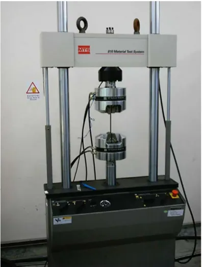
The study used Max. Load of tensile-shear test specimens as the quality characteristic in the process. A universal testing machine as shown in Fig.2-6

(37)

had been used for this study to measure the Max. Load of the RSW specimens. The speed was set at 0.1 mm sec-1 in the testing.

Fig. 2-6Universal testing machine used

As learned from handbook and the practical experience in the production of auto-body, the major welding parameters for the processing quality of weldment include welding current, welding time, electrode force, the size of electrode tip, and surface condition of specimens in the RSW process.

(38)

CHAPTER 3 EXPERIMENTAL PROCEDURES

3.1 Proposed procedure

Select a welding process

Taguchi method for initial optimization Control factor& Noise factor Orthogoral array (Modify) Experimental results Evaluation ANOVA Confirmation Neural network for real optimization Training of BP network Select a well- trained network Optimization via a well-trained network

(39)

In this dissertation, the proposed approach consists of two phases. Phase 1 executes initial optimization via Taguchi method to construct a database for the neural network. Phase 2 applies a neural network with the Levenberg-Marquardt back-propagation (LMBP) algorithm to search for the optimal parameter combination. Three examples involving the gas tungsten arc (GTA) welding, the pulsed Nd:YAG laser micro-weld process, and the resistance spot welding (RSW) process in automotive industry demonstrate the effectiveness of the proposed approach.

3.2 Optimization for GTA welding

3.2.1 Initial optimization for GTA welding

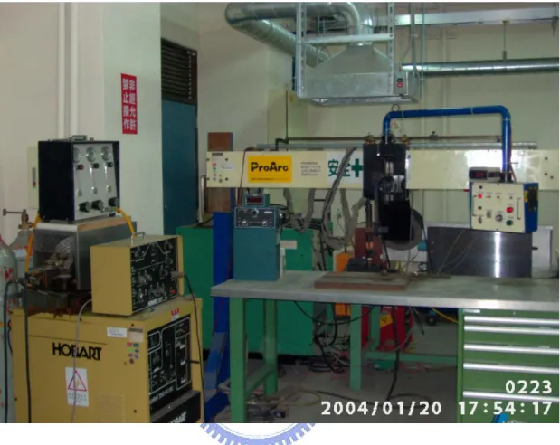
JIS SUS 304 stainless steel was used in this study with its chemical composition being listed in Table 3-1. The test specimens had the dimensions 50 ×100×2.8 ㎜. Autogenous (no filler metal was added) and GTA welding was conducted using an EWTh-2 electrode to produce a bead-on-plate weld. A servomechanism controlled the traveling speed of the electrode. The GTA welder (HORBART TIGWAVETM 350AC/DC type ) has been utilized for the experiment, as shown in Fig.3-1.

Table 3-1 Material used in GTA welding (wt-%)

Material C Si Mn P S Cr Ni Fe

JIS SUS 304

(40)

Fig. 3-1 The equipment of Autogenous GTA welder

As shown in Fig.2-1, the W and D value of the specimens of type A were measured by a Nonus (Pierre Vernier) with 0.02 ㎜ precision. An optical microscope was used to measure the specimens of Type B. All metallographic specimens were prepared by mechanical lapping, grinding, and polishing to 0.3 μm finish, followed by etching in a solution of 10g.CuSO4＋50ml.HCl＋

(41)

Control and noise factor of the GTA welding

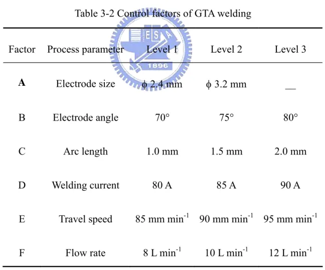
Taguchi separates factors into two main groups, the control factor and noise factor. Control factors are those that allow a manufacturer to control during processing and the noise factors are expensive and difficult to control [10]. Welding current, travel speed of the welding torch, arc length, flow rate of the shielding gas, electrode size and its angle were selected as the controlling factors. The value of each welding process parameter at the different levels is listed in Table 3-2.

Table 3-2 Control factors of GTA welding

Factor Process parameter Level 1 Level 2 Level 3

A Electrode size φ 2.4 mm φ 3.2 mm __

B Electrode angle 70° 75° 80°

C Arc length 1.0 mm 1.5 mm 2.0 mm

D Welding current 80 A 85 A 90 A

E Travel speed 85 mm min-1 90 mm min-1 95 mm min-1

(42)

The fundamental principle of Robust Design is to improve the quality by minimizing the effect of the causes of variation. It is important in every Robust Design project to identify important noise factors [10]. Engineering experience and judgment are needed in identifying the noise factor. Cleanliness of the weld joint areas was selected as the noise factor in this study. The surface impurities were removed and cleaned with acetone at level one (N1). The specimens at level two (N2) without any cleaning treatment may have been tarnished with dirt and / or grease.

Orthogonal array experiment

One two-level and five three-level control factors in addition to one noise factor were considered in this investigation. The interaction effect between the welding parameters was not considered. Therefore, there are 11 degrees of freedom owing to the 6 control factors. The degrees of freedom for the OA should be greater than or at least equal to those for the process parameters. The standard arrays available are L18 and L27. L18 has 8 columns, but provides low

resolution. The L27 has 13 columns with greater resolution than L18. L27 (313) OA

was employed in this study.

The “dummy level technique ” was then used for modifying L27 (313) OA

into L27 (21×35) OA. The control factor A was assigned to the column 1 of L27

OA by using dummy levels A3=A2′. Other control factors (B~F) were assigned

to the column 2 ~ 6. An experimental layout with an inner array for control factors and an outer array for a two-level noise factor (N1 and N2) is shown in Table 3-3.

(43)

are planned in this experimental arrangement. In the Taguchi method, repetitions are used to assess the noise effect on some quality characteristic(s) of interest. Fig.3-2 shows the measuring procedure of weld pool geometry.

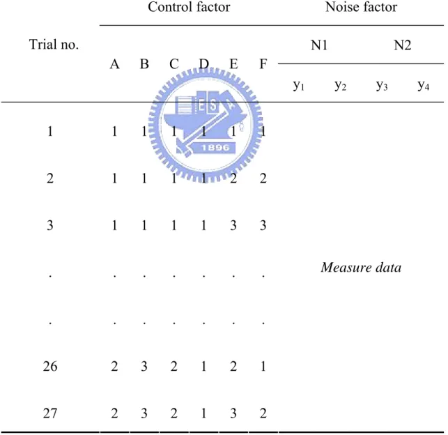
Table 3-3 Experimental layout using an L27 orthogonal array

Control factor Noise factor

N1 N2 Trial no. A B C D E F y1 y2 y3 y4 1 1 1 1 1 1 1 2 1 1 1 1 2 2 3 1 1 1 1 3 3 . . . . . . . . 26 2 3 2 1 2 1 27 2 3 2 1 3 2 Measure data

(44)

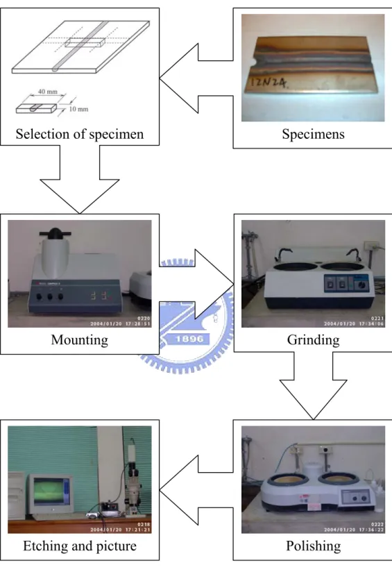
Fig. 3-2 Measurement of weld pool geometry Specimens Mounting Selection of specimen Grinding Polishing Etching and picture

(45)

Evaluation of initial optimal condition

The depth-to-width ratios (DWR) of the weld pool geometry as discussed earlier belong to the higher-is-better quality characteristic. The S/N ratios, which condense the multiple data points within a trial, depend on the type of characteristic being evaluated. The equation for calculating S/N ratio for HB characteristic is ⎟⎟ ⎠ ⎞ ⎜⎜ ⎝ ⎛ − =

∑

= n i yi n N S 1 2 10 1 1 log 10 / 3-1

where n is the number of tests in a trial (number of repetitions regardless of

noise levels). The value of n is 4 in this study. The S/N ratio corresponding to

the D/W ratio of each trial is shown in Table 3-4. The effect of each welding process parameter on the S/N ratio at different levels can be separated out because the experimental design is orthogonal. The description of the S/N ratio for each level of the welding process parameters is summarized and shown in Table 3-5.

(46)

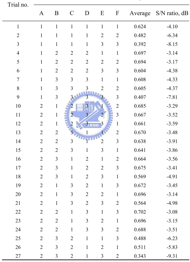
Table 3-4 Summary of experiment data of GTA welding

Control factors Depth-to-width ratio Trial no. A B C D E F Average S/N ratio, dB 1 1 1 1 1 1 1 0.624 -4.10 2 1 1 1 1 2 2 0.482 -6.34 3 1 1 1 1 3 3 0.392 -8.15 4 1 2 2 2 1 1 0.697 -3.14 5 1 2 2 2 2 2 0.694 -3.17 6 1 2 2 2 3 3 0.604 -4.38 7 1 3 3 3 1 1 0.608 -4.33 8 1 3 3 3 2 2 0.605 -4.37 9 1 3 3 3 3 3 0.407 -7.81 10 2 1 2 3 1 2 0.685 -3.29 11 2 1 2 3 2 3 0.667 -3.52 12 2 1 2 3 3 1 0.661 -3.59 13 2 2 3 1 1 2 0.670 -3.48 14 2 2 3 1 2 3 0.638 -3.91 15 2 2 3 1 3 1 0.641 -3.86 16 2 3 1 2 1 2 0.664 -3.56 17 2 3 1 2 2 3 0.675 -3.41 18 2 3 1 2 3 1 0.569 -4.91 19 2 1 3 2 1 3 0.672 -3.45 20 2 1 3 2 2 1 0.696 -3.14 21 2 1 3 2 3 2 0.564 -4.98 22 2 2 1 3 1 3 0.702 -3.08 23 2 2 1 3 2 1 0.696 -3.15 24 2 2 1 3 3 2 0.688 -3.51 25 2 3 2 1 1 3 0.488 -6.23 26 2 3 2 1 2 1 0.511 -5.83 27 2 3 2 1 3 2 0.343 -9.31

(47)

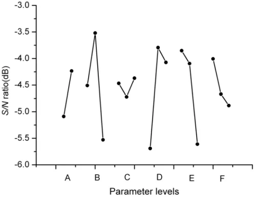
Table 3-5 S/N response table for the weld pool geometry

Factor Process parameter Level 1 Level 2 Level 3

A Electrode size – 5.088 – 4.234 __ B Electrode angle – 4.508 – 3.520 – 5.529 C Arc length – 4.467 – 4.719 – 4.370 D Welding current – 5.691 – 3.794 – 4.072 E Travel speed – 3.851 – 4.095 – 5.611 F Flow rate – 4.006 – 4.669 – 4.882

Fig.3-3 shows the S/N ratio graph that the data obtained from Table 3-5. Basically, the larger is the S/N ratio, the better the quality characteristic (depth-to-width ratio) is for the weld pool geometry. The initial optimal combinations of the GTA welding process parameter levels, A2B2C3D2E1F1, can

(48)

Fig. 3-3 S/N graph for the weld pool geometry

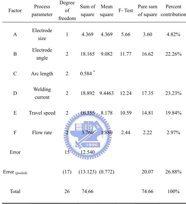
The electrode angle, welding current, travel speed, and arc length were the significant welding parameters in affecting the quality characteristic, with the welding current and electrode angle being the most significant, as indicated from Table 3-6.

(49)

Table 3-6 Results of ANOVA for the weld pool geometry Factor Process parameter Degree of freedom Sum of square Mean square F- Test Pure sum of square Percent contribution A Electrode size 1 4.369 4.369 5.66 3.60 4.82% B Electrode angle 2 18.165 9.082 11.77 16.62 22.26% C Arc length 2 0.584 * D Welding current 2 18.892 9.4463 12.24 17.35 23.23% E Travel speed 2 16.355 8.178 10.59 14.81 19.84% F Flow rate 2 3.760 1.880 2.44 2.22 2.97% Error 15 12.540 Error (pooled) (17) (13.123) (0.772) 20.07 26.88% Total 26 74.66 74.66 100%

Mark *means the factors are treated as pooled error

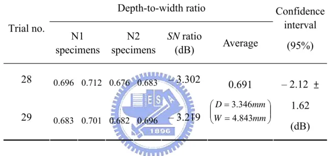
Confirmation tests

An interval confidence of 95% for the depth-to-width ratio, the F₀_.₀₅_;₁_;₁₇

=4.45, Vep=0.772, the sample size for the confirmation experiment r is 2,

(50)

confidence interval is computed as CI =1.62(dB). The experimental results (Table 3-7) confirm that the initial optimizations of the GTA welding process parameters were achieved.

Table 3-7 Confirmation experiment of GTA welding Depth-to-width ratio Trial no. N1 specimens N2 specimens SN ratio (dB) Average Confidence interval (95%) 28 _{0.696 0.712 0.676 0.683} – 3.302 29 _{0.683 0.701 0.682 0.696} – 3.219 0.691 ⎟⎟ ⎠ ⎞ ⎜⎜ ⎝ ⎛ = = mm W mm D 843 . 4 346 . 3 – 2.12 ± 1.62 (dB)

3.2.2 Real optimization for GTA welding

Training of BP network

A feed-forward neural network is proposed for this study. It takes a set of six input values (control factors A, B, C, D, E, and F) and predicts the value of two outputs (D and W value of the weld pool geometry). A total of 108 input-output data patterns were partitioned into a training set and a testing set. Functionally, 80% (approximately 87 patterns) were randomly selected for training the neural network while the remaining 20% (approximately 21 patterns)

(51)

algorithm, was used to improve classical back-propagation learning in the training process. Table 3-8 presents eight options of the neural network architecture. Under the less simulating error that compared with average value of W and D in Table 7 and best convergence criterion of the mean square error (MSE) of the testing subset, the structure 6-7-2 was selected to obtain a better performance. The topology of the network 6-7-2 with a 0.001 μ value and a θ

value of 10 is depicted in Fig.3-4.

Table 3-8 Options for different networks in GTA welding Simulating error, % (Compare with average value

in Table 3-7) Architecture

(Input-hidden unit-output) MSE for training

W value D value 6-2-2 0.057447 –4.65 0.29 6-3-2 0.043527 2.01 5.82 6-4-2 0.043214 – 5.28 1.36 6-5-2 0.073604 0.53 8.54 6-6-2 0.023242 – 59.32 – 21.84 6-7-2 0.041730 – 1.44 5.28 6-8-2 0.044620 – 8.34 0.36 6-9-2 0.011117 36.05 13.15

(52)

Fig. 3-4 The BP network topology of the GTA welding process

Optimization with trained network

The control factor B (electrode angle) and D (welding current) are the significant welding parameters in affecting the quality characteristic (depth-to-width ratio of each weldment) as shown in Table 3-6. The trained network 6-7-2 was employed as the simulating function of the primary parameters in this welding process. Fig.3-5 shows the comparison of simulating results using the significant welding parameters (factor B and D) obtained by the Taguchi method, from which it can be seen that the depth-to-width ratio of weld pool geometry is best for adjusting welding current to 81 A and electrode to 73 degree of angle.

(53)

Fig. 3-5 Simulation different electrode angle and welding current

3.3 Optimization for Nd:YAG laser micro-weld

3.3.1 Initial optimization for Nd:YAG laser micro-weld

The materials of safety vent and cathode lead used for lithium-ion secondary batteries are AA3003 aluminum alloy (Please refer to Table 3-9 for its chemical composition). The safety vent had the dimensions φ18×1.0 mm; cathode lead had the dimensions 3×70×0.1 mm. The pulsed Nd:YAG laser spot welder (Toshiba Lay-822H type) has been utilized for the experiment. The wavelength of laser is 1.06 μm and through the fiber conduction, the laser beam is to joint the product, as shown in Fig.3-6. Fig.3-7 shows the illustration of automatic mass production for the lithium-ion secondary battery parts (safety vent and cathode lead).

(54)

Table 3-9 Material used in Nd:YAG laser spot welding (wt-%)

Material Si Cu Mn Zn Others Al

AA3003

Aluminum Alloy 0.7 0.05~0.2 1.0~1.5 0.1 0.15 Balance

(55)

(56)

The Max. Load of weldment lower than 0.5 kg were determined to defective products, as suggested by the engineers of a manufacturing lithium-ion secondary batteries company in Taiwan. To prevent leakage from “safety vent”, Max. Load was restricted under 1.2 kg. In practice, the higher energy of pulsed Nd:YAG laser welding (e.g., higher pulse peak value), the deeper penetration of weldment being obtained. The deeper penetration of weldment (between “safety vent” and “cathode lead”) would be increasing the Max. Load. However, it may be pierce through the “safety vent” and result in leakage of lithium-ion secondary batteries in the future. Summary, increasing Max. Load of weldment to 1.0 kg and decreasing the defective rate under 5% is attempted in this study.

Control and noise factor of Nd:YAG laser micro-weld

As learned from the literature [43] and the experience in the production process of lithium-ion secondary batteries, the major welding parameters for the pulsed Nd:YAG laser spot welding quality of weldment include pulse peak value, pulse width, pulse frequency and focus position. The parameters as mentioned above may be respectively adjusted within the range as below: pulse peak value 0 ~ 500 Volt, pulse width 0.2 ~ 20.0 msec, pulse frequency 0.5 ~ 20 pps and focus position –1.0 ~ +1.0 mm. The values of the welding process parameters at the different levels are listed in Table 3-10.

Aluminum and its alloys have high reflectivity together with large thermal conductivity; it is a poor absorber of laser light. Laser welding of aluminum and its alloys is difficult and the weld quality is often very poor [37,38]. Another problem that adversely affects welding of aluminum and its alloys is the natural oxide and other contamination on the material surface. So, the cleaning

(57)

treatment on “safety vent” and “cathode lead” of lithium-ion secondary batteries (AA3003 aluminum alloy) surface is very important. Unfortunately, it is very hard to control the surface cleanliness of the weldment in the automatic mass production. Thus, cleanliness of the weld joint areas was selected as the noise factor of Taguchi method in this study. The surface impurities were removed and the surface was cleaned with acetone at level one (N1, 100% cleanliness). The specimens at level two (N2, 0% cleanliness), without any cleaning treatment, may have been tarnished with dirt and / or grease.

Table 3-10 Control factors of Nd:YAG laser spot welding

Factor _parameterProcess Level 1 Level 2 Level 3 Level 4 Level 5

A Focus position

(㎜) – 0.5 0 + 0.5 __ __

B Pulse peak value

(Volt.) 300 315 330 345 360

C Pulse width

(msec) 4 5 6 7 8

D Pulse frequency

(58)

Orthogonal array experiment

One tree-level and tree five-level control factors, in addition to one noise factor, were considered in this investigation. The interaction effect between the welding parameters was not considered. Therefore, there are 14 degrees of freedom, owing to the four control factors. The degrees of freedom for the OA should be greater than or at least equal to those for the process parameters. The L25 (56) OA was employed in this study. The ‘dummy level technique’ was then

used for changing the L25 (56) OA into the L25 (31×53) OA. Control factor A was

assigned to the column 1 of L25 OA by using dummy levels A2=A1′, A3=A2′,

A4=A3′ and A5=A3′. Other control factors (B~D) were assigned to the column 2

~ 4. Note that the orthogonality was preserved even when the dummy level technique was applied to one or more factors.

In addition, the noise factor could be assigned to the outer array to determine some level of a control factor that does not give much variation in the results, even though a noise factor is definitely present. An experimental layout with an inner array for control factors and an outer array for a two-level noise factor (N1 and N2) is shown in Table 3-11. There are 25×2=50 separate test conditions; four repetitions for each trial (y1, y2, y3 and y4) were planned in this

experimental arrangement; y1 and y2 are N1 specimens (cleaned with acetone), y3

and y4 are N2 specimens (without cleaning). In the Taguchi method, repetitions

(59)

Table 3-11 Experimental layout using L25 orthogonal array

Control factor Noise factor

N1 specimens N2 specimens Trial no. _{A B C D} y1 y2 y3 y4 1 1 1 1 1 2 1 2 2 2 3 1 3 3 3 4 1 4 4 4 5 1 5 5 5 6 1 1 2 3 7 1 2 3 4 8 1 3 4 5 9 1 4 5 1 10 1 5 1 2 11 2 1 3 5 12 2 2 4 1 13 2 3 5 2 14 2 4 1 3 15 2 5 2 4 16 3 1 4 2 17 3 2 5 3 18 3 3 1 4 19 3 4 2 5 20 3 5 3 1 21 3 1 5 4 22 3 2 1 5 23 3 3 2 1 24 3 4 3 2 25 3 5 4 3 Measure data

(60)

Evaluation of initial optimal condition

The tensile-shear strength of the specimens, as discussed earlier, belongs to the HB quality characteristic. The SNRs, which condense the multiple data points within a trial, depend on the type of characteristic being evaluated. The equation for calculating the SNR ratio for HB characteristic is

2 1 1 1 10log n i i SNR n = y ⎛ ⎞ = − _⎜ _⎟ ⎝

∑

⎠ 3-2

where n is the number of tests in a trial (number of repetitions regardless of

noise levels) and yi is the Max. Load of each specimens. The value of n is 4

in this study. The SNR corresponding to Max. Load of each trial is shown in Table 3-12. The effect of each welding process parameter on the SNR at different levels can be separated out because the experimental design is orthogonal. The description of the SNR for each level of the welding process is summarized in Table 3-13. Fig.3-8 shows the SNR graph obtained from Table 3-13. Basically, the larger the SNR, the better the quality characteristic (tensile-shear strength) is for the specimens. The initial optimal combinations of the pulsed Nd:YAG laser micro-weld process parameter levels, A3B5C3D5, can

(61)

Table 3-12 Experiment data of Nd:YAG laser micro-weld Max. Load, kg Trial no. y1 y2 y3 y4 Average SNR, dB 1 0.05 0.10 0.01 0.01 0.04 –37.10 2 0.20 0.25 0.10 0.15 0.18 –16.66 3 0.70 0.64 0.50 0.40 0.56 –5.66 4 0.75 0.80 0.65 0.70 0.73 –2.87 5 0.85 1.00 0.80 0.75 0.85 –1.56 6 0.20 0.20 0.15 0.10 0.16 –16.87 7 0.35 0.55 0.30 0.45 0.41 –8.38 8 0.70 0.80 0.50 0.65 0.66 –3.97 9 0.40 0.25 0.35 0.20 0.30 –11.42 10 0.35 0.40 0.45 0.30 0.38 –8.82 11 0.25 0.20 0.20 0.15 0.20 –14.41 12 0.20 0.35 0.20 0.30 0.26 –12.39 13 0.15 0.20 0.15 0.10 0.15 –17.28 14 0.65 0.50 0.35 0.50 0.50 –6.66 15 0.50 0.65 0.40 0.60 0.54 –5.85 16 0.25 0.05 0.15 0.10 0.14 –21.46 17 0.30 0.35 0.40 0.20 0.31 –11.01 18 1.00 0.90 0.60 0.40 0.73 –4.50 19 0.60 0.70 0.50 0.65 0.61 –4.47 20 0.85 0.90 0.70 0.90 0.84 –1.68 21 0.35 0.30 0.10 0.20 0.24 –15.57 22 0.45 0.40 0.30 0.50 0.41 –8.18 23 0.55 0.50 0.35 0.50 0.48 –6.87 24 0.80 0.70 0.60 0.75 0.71 –3.10 25 0.80 0.95 0.70 0.85 0.83 –1.83 Total average of SNR for all trial is –9.942 (dB)

(62)

Table 3-13 SNR response table for the quality characteristic

Factor Process

parameter Level 1 Level 2 Level 3 Level 4 Level 5

A Focus position –11.329 –11.318 –7.867 – – B Pulse peak value –21.082 –11.323 –7.656 –5.701 –3.948 C Pulse width –13.049 –10.144 –6.646 –8.503 –11.368 D Pulse frequency –13.891 –13.464 –8.406 –7.433 –6.516

(63)

The pulse peak value, pulse frequency and focus position were the significant welding parameters affecting the quality characteristic (tensile-shear strength of each specimen), with the pulse peak value being the most significant, as indicated by Table 3-14.

Table 3-14 Results of ANOVA for the quality characteristic

Factor Process parameter Degree of freedom Sum of square Mean square F- test Pure sum of square Percent contribution A Focus position 2 196.049 98.025 19.75 186.12 12.11% B Pulse peak value 4 925.757 231.439 46.63 905.90 58.95% C Pulse width 4 123.328 30.832 6.21 103.47 6.73% D Pulse frequency 4 241.943 60.486 12.19 222.09 14.45% Error 10 49.636 4.964 119.13 7.75% Total 24 1536.71 1536.71 100%

(64)

Confirmation tests for initial optimization

Refer to Table 3-13 and 3-14, the factor C shows the least effect for quality characteristic. In order to prevent over-estimate [8], factor C is not considered, the estimated SNR ηopt is computed as

opt

η = –9.942+(–7.867+9.942) +(–3.948+9.942) +(–6.516+9.942) =1.553 (dB)

With CI of 95% for the tensile-shear strength, the F₀_.₀₅_,₁_,₁₀ =4.96 and

ep

V =4.964, the sample size for the confirmation experiment r is 3, N =25,

opt

DOF =10, and the effective sample size n_eff is 2.273. Thus, the CI is

computed to be CI=4.364 (dB). The experimental results (Table 3-15) confirm

that the initial optimizations of the Nd:YAG laser micro-weld process parameters were achieved.

Table 3-15Confirmation experiment of Nd:YAG laser micro-weld

Max. Load Trial no. N1 specimens N2 specimens SNR, dB Average, kg Confidence interval, 95% 26 0.96 1.05 0.83 0.92 – 0.63 27 1.05 1.00 0.90 0.83 – 0.60 28 1.02 0.97 0.82 0.85 – 0.88 0.933 N1=1.008 N2=0.858 1.553 ± 4.364 (dB)

(65)

3.3.2 Real optimization for Nd:YAG micro-weld

Training of BP network

A feed-forward neural network is proposed for this study. It takes a set of five input values (control factors A, B, C, D and noise factor) and predicts the value of one output (Max. Load of the specimens). A total of 100 input-output data patterns were partitioned into a training set, a testing set and a validating set. Functionally, 60% (60 patterns) were randomly selected for training the neural network the remaining 20% (20 patterns) were randomly used for testing and 20% (20 patterns) were randomly used for validating. An efficient algorithm, the Levenberg-Marquardt algorithm, was used to improve classical BP learning in the training process [17,21]. The neural network package software MATLAB Neural Network ToolBox was used to develop the required network.

Table 3-16 presents fifteen options for the neural network architecture. After comparing all the data for the mean square error (MSE), the structure 5-3-1, 5-15-1, 5-25-1, 5-35-1 and 5-40-1 are the five best convergence criteria. The structure 5-15-1 showed the least error and was therefore selected to obtain a better performance. The topology of the network 5-15-1 with a μ value 0.001 and a θ value of 10 is shown in Fig. 3-9.

(66)

Table 3-16 Options for different networks in Nd:YAG laser welding Simulating error, %

(Compare with average value in Table 3-15) Architecture (input-hidden unit-output) Mean square error for training N1 value N2 value 5-2-1 0.0077 –20.6 –16.6 5-3-1* 0.0046 –26.2 –19.1 5-4-1 0.0121 –14.1 –8.2 5-5-1 0.0052 –21.3 –21.4 5-6-1 0.0078 –21.9 –10.5 5-7-1 0.0304 –25.0 –37.9 5-8-1 0.0119 –31.6 –29.7 5-9-1 0.0064 –24.5 –24.3 5-10-1 0.0083 –16.0 –22.6 5-15-1* 0.0027 5.1 –13.1 5-20-1 0.0099 –33.2 –19.0 5-25-1* 0.0027 –33.7 –62.2 5-30-1 0.0243 –50.9 83.2 5-35-1* 0.0034 –22.9 –33.4 5-40-1* 0.0020 –20.8 –50.6